Full Terms & Conditions of access and use can be found at
http://www.tandfonline.com/action/journalInformation?journalCode=ubes20
Download by: [Universitas Maritim Raja Ali Haji] Date: 13 January 2016, At: 00:33
Journal of Business & Economic Statistics
ISSN: 0735-0015 (Print) 1537-2707 (Online) Journal homepage: http://www.tandfonline.com/loi/ubes20
Out-of-Sample Performance of Discrete-Time Spot
Interest Rate Models
Yongmiao Hong, Haitao Li & Feng Zhao
To cite this article: Yongmiao Hong, Haitao Li & Feng Zhao (2004) Out-of-Sample Performance
of Discrete-Time Spot Interest Rate Models, Journal of Business & Economic Statistics, 22:4, 457-473, DOI: 10.1198/073500104000000433
To link to this article: http://dx.doi.org/10.1198/073500104000000433
View supplementary material
Published online: 01 Jan 2012.
Submit your article to this journal
Article views: 75
View related articles
Out-of-Sample Performance of Discrete-Time
Spot Interest Rate Models
Yongmiao HONG
Department of Economics and Department of Statistical Sciences, Cornell University, Ithaca, NY 14850 Department of Economics, Tsinghua University, Beijing, China 100084 (yh20@cornell.edu)
Haitao LI
Johnson Graduate School of Management, Cornell University, Ithaca, NY 14850 (hl70@cornell.edu)
Feng ZHAO
Department of Economics, Cornell University, Ithaca, NY 14850 (fz17@cornell.edu)
We provide a comprehensive analysis of the out-of-sample performance of a wide variety of spot rate models in forecasting the probability density of future interest rates. Although the most parsimonious models perform best in forecasting the conditional mean of many financial time series, we find that the spot rate models that incorporate conditional heteroscedasticity and excess kurtosis or heavy tails have better density forecasts. Generalized autoregressive conditional heteroscedasticity significantly improves the modeling of the conditional variance and kurtosis, whereas regime switching and jumps improve the modeling of the marginal density of interest rates. Our analysis shows that the sophisticated spot rate models in the existing literature are important for applications involving density forecasts of interest rates.
KEY WORDS: Density forecast; Generalized autoregressive conditional heteroscedasticity; General-ized spectrum; Jumps; Parameter estimation uncertainty; Regime switching.
1. INTRODUCTION
The short-term interest rate plays an important role in many areas of asset pricing studies. For example, the instantaneous risk-free interest rate, or the so-called “spot rate,” is the state variable that determines the evolution of the yield curve in the well-known term structure models of Vasicek (1977) and Cox, Ingersoll, and Ross (CIR) (1985). The spot rate is thus of fun-damental importance to the pricing of fixed-income securities and the management of interest rate risk. Many interest rate models have been proposed, and over the last decade, a vast body of literature has been developed to rigorously estimate and test these models using high-quality interest rate data. (See, e.g., Chapman and Pearson 2001 for a survey of the empiri-cal literature.)
Despite the progress that has been made in modeling interest rate dynamics, most existing studies have typically focused on the in-sample fit of historical interest rates and ignored out-of-sample forecasts of future interest rates. In-out-of-sample diagnostic analysis is important and can reveal useful information about possible sources of model misspecifications. In many financial applications, such as the pricing and hedging of fixed-income securities and the management of interest rate risk, however, what matters most is the evolution of the interest rate in the future, not in the past.
In general, there is no guarantee that a model that fits his-torical data well will also perform well out-of-sample due to at least three important reasons. First, the extensive search for more complicated models using the same (or similar) dataset(s) may suffer from the so-called “data-snooping bias,” as pointed out by Lo and MacKinlay (1989) and White (2000). A more-complicated model can always fit a given dataset better than simpler models, but it may overfit some idiosyncratic features of the data without capturing the true data-generating process.
Out-of-sample evaluation will alleviate, if not eliminate com-pletely, such data-snooping bias. Second, an overparameterized model contains a large number of estimated parameters and in-evitably exhibits excessive sampling variation in parameter es-timation, which in turn may adversely affect the out-of-sample forecast performance. Third, a model that fits a historical dataset well may not forecast the future well because of unfore-seen structural changes or regime shifts in the data-generating process. Therefore, from both practical and theoretical stand-points, in-sample analysis alone is not adequate, and it is nec-essary to examine the out-of-sample predictive ability of spot rate models.
We contribute to the literature by providing the first com-prehensive empirical analysis (to our knowledge) of the out-of-sample performance of a wide variety of popular spot rate models. Although some existing studies (e.g., Gray 1996; Bali 2000; Duffee 2002) have conducted out-of-sample analysis of interest rate models, what distinguishes our study is that we focus on forecasting the probability density of future interest rates, rather than just the conditional mean or the first few conditional moments. This distinction is important because in-terest rates, like most other financial time series, are highly non-Gaussian. Consequently, one must go beyond the condi-tional mean and variance to get a complete picture of interest rate dynamics. The conditional probability density character-izes the full dynamics of an interest rate model and thus es-sentially checks all conditional moments simultaneously (if the moments exist).
Density forecasts are important not only for statistical evalua-tion, but also for many economic and financial applications. For
© 2004 American Statistical Association Journal of Business & Economic Statistics October 2004, Vol. 22, No. 4 DOI 10.1198/073500104000000433
457
example, the booming industry of financial risk management is essentially dedicated to providing density forecasts for impor-tant economic variables and portfolio returns, and to tracking certain aspects of distribution, such as value at risk (VaR), to quantify the risk exposure of a portfolio (e.g., Morgan 1996; Duffie and Pan 1997; Jorion 2000). More generally, modern risk control techniques all involve some form of density fore-cast, the quality of which has real impact on the efficacy of capital asset/liability allocation. In macroeconomics, monetary authorities in the United States and United Kingdom (the Fed-eral Reserve Bank of Philadelphia and the Bank of England) have been conducting quarterly surveys on density forecasts for inflation and output growth to help set their policy instru-ments (e.g., inflation target). There is also a growing literature on extracting density forecasts from options prices to obtain useful information on otherwise unobservable market expecta-tions (e.g., Fackler and King 1990; Jackwerth and Rubinstein 1996; Soderlind and Svensson 1997; Ait-Sahalia and Lo 1998). In the recent development of time series econometrics, there is a growing interest in out-of-sample probability distribution forecasts and their evaluation, motivated from the context of decision-making under uncertainty. Important works in this area include those of Bera and Ghosh (2002), Berkowitz (2001), Christoffersen and Diebold (1996, 1997), Clements and Smith (2000), Diebold, Gunther, and Tay (1998), Diebold, Hahn, and Tay (1999), Diebold, Tay, and Wallis (1999), Granger (1999), and Granger and Pesaran (2000). One of the most important is-sues in density forecasting is to evaluate the quality of a forecast (Granger 1999). Suboptimal density forecasts will have real ad-verse impact in practice. For example, an excessive forecast for VaR would force risk managers and financial institutions to hold too much capital, imposing an additional cost. Suboptimal den-sity forecasts for important macroeconomic variables may lead to inappropriate policy decisions (e.g., inappropriate level and timing in setting interest rates), which could have serious con-sequences for the real economy.
Evaluating density forecasts, however, is nontrivial, sim-ply because the probability density function of an underly-ing process is not observable even ex post. Unlike for point forecasts, there are few statistical tools for evaluating density forecasts. In a pioneering contribution, Diebold et al. (1998) evaluated density forecast by examining the probability inte-gral transforms of the data with respect to a density forecast model. Such a transformed series is often called the “gener-alized residuals” of the density forecast model. It should be iid U[0,1]if the density forecast model correctly captures the full dynamics of the underlying process. Any departure from iid U[0,1] is evidence of suboptimal density forecasts and model misspecification.
Diebold et al. (1998) used an intuitive graphical method to separately examine the iid and uniform properties of the “gener-alized residuals.” This method is simple and informative about possible sources of suboptimality in density forecasts. Hong (2003) recently developed an omnibus evaluation procedure for density forecasts by measuring the departure of the “general-ized residuals” from iid U[0,1]. The evaluation statistic pro-vides a metric of the distance between the density forecast model and the true data-generating process. The most appeal-ing feature of this new test is its omnibus ability to detect a
wide range of suboptimal density forecasts, thanks to the use of the generalized spectrum. The latter was introduced by Hong (1999) as an analytic tool for nonlinear time series and is based on the characteristic function in a time series context. There has been an increasing interest in using the characteristic function in financial econometrics (see, e.g., Chacko and Viceira 2003; Ghysels, Carrasco, Chernov, and Florens 2001; Hong and Lee 2003a,b; Jiang and Knight 1997; Singleton 2001).
Applying Hong’s (2003) procedure, we provide a compre-hensive empirical analysis of the density forecast performance of a variety of popular spot rate models, including single-factor diffusion, generalized autoregressive conditional heteroscedas-ticity (GARCH), regime-switching, and jump-diffusion models. The in-sample performance of these models has been exten-sively studied, but their out-of-sample performance, especially their density forecast performance is still largely unknown. We find that although previous studies have shown that sim-pler models, such as the random walk model, tend to provide better forecasts for the conditional mean of many financial time series, including interest rates and exchange rates (e.g., Duffee 2002; Meese and Rogoff 1983), more-sophisticated spot rate models that capture volatility clustering, and excess kurtosis and heavy tails of interest rates have better density forecasts. GARCH significantly improves the modeling of the dynam-ics of the conditional variance and kurtosis of the generalized residuals, whereas regime switching and jumps significantly improve the modeling of the marginal density of interest rates. Our analysis shows that the sophisticated spot rate models in the existing literature can indeed capture some important fea-tures of interest rates and are relevant to applications involving density forecasts of interest rates.
The article is organized as follows. In Section 2 we discuss the methodology for density forecast evaluation. In Section 3 we introduce a variety of popular spot rate models. In Section 4 we describe data, estimation methods, and the in-sample per-formance of each model. In Section 5 we subject each model to out-of-sample density forecast evaluation, and in Section 6 we provide concluding remarks. In the Appendix we discuss Hong’s (2003) evaluation procedure for density forecasts.
2. OUT–OF–SAMPLE DENSITY FORECAST EVALUATION
The probability density function is a well-established tool for characterizing uncertainty in economics and finance (e.g., Rothschild and Stiglitz 1970). The importance of density fore-casts has been widely recognized in recent literature due to the works of Diebold et al. (1998), Granger (1999), and Granger and Pesaran (2000), among many others. These authors showed that accurate density forecasts are essential for decision mak-ing under uncertainty when the forecaster’s objective function is asymmetric and the underlying process is non-Gaussian. In a decision-theoretic context, Diebold et al. (1998) and Granger and Pesaran (2000) showed that if a density forecast coincides with the true conditional density of the data generating process, then it will be preferred by all forecast users regardless of their objective functions (e.g., risk attitudes). Thus testing the opti-mality of a forecast boils down to checking whether the density forecast model can capture the true data-generating process.
This is a challenging job, because we never observe an ex post density. So far there are few statistical evaluation procedures for density forecasts.
Diebold et al. (1998) used the probability integral transform of data with respect to the density forecast model to assess the optimality of density forecasts. Extending a result established by Rosenblatt (1952), they showed that if the model conditional density is specified correctly, then the probability integral trans-formed series should be iid U[0,1].
Specifically, for a given model of interest ratert, there is a
model-implied conditional density
∂
∂rP(rt≤r|It−1, θ )=p(r,t|It−1, θ ),
where θ is an unknown finite-dimensional parameter vector and It−1 ≡ {rt−1, . . . ,r1} is the information set available at
timet−1. Suppose that we have a random sample {rt}Nt=1of
size N, which we divide into two subsets, an estimation sam-ple{rt}Rt=1 of sizeRand a prediction sample{rt}Nt=R+1 of size
n=N−R. We can then define the dynamic probability inte-gral transform of the data{rt}Nt=R+1 with respect to the model
Suppose that the model is correctly specified in the sense that there exists some θ0 such that p(r,t|It−1, θ0) coincides with
the true conditional density of rt. Then the transformed
se-quence{Zt(θ0)}is iid U[0,1].
For example, consider the discretized Vasicek model
rt=α0+α1rt−1+σzt,
ditional density ofrt. Then
Zt(θ0)=
sistent estimator for θ0. This series provides a convenient
ap-proach for evaluating the density forecast modelp(r,t|It−1, θ ).
Intuitively, the U[0,1]property characterizes the correct spec-ification for the stationary distribution of {rt}, and the iid
property characterizes correct dynamic specification for {rt}.
If{Zt(θ )}is not iid U[0,1]for allθ, then the density forecast
modelp(r,t|It−1, θ )is not optimal, and there is room for
fur-ther improvement.
To test the joint hypothesis of iid U[0,1]for{Zt(θ )}is
non-trivial. One may suggest using the well-known Kolmogorov– Smirnov test, which unfortunately checks U[0,1] under the
iid assumption rather than checking iid U[0,1]jointly. It will miss the alternatives for which{Zt(θ )}is uniform, but not iid.
Similarly, tests for iid alone will miss the alternatives for which
{Zt(θ )}is iid but not U[0,1]. Moreover, parameter estimation
uncertainty is expected to affect the asymptotic distribution of the Kolmogorov–Smirnov test statistic.
Diebold et al. (1998) used the autocorrelations ofZm t (θ )ˆ to
check the iid property and the histogram of Zt(θ )ˆ to check
the U[0,1] property. These graphical procedures are simple and informative. To compare and rank different models, how-ever, it is desirable to use a single evaluation criterion. Hong (2003) recently developed an omnibus evaluation procedure for out-of-sample density forecast that tests the joint hypothesis of iid U[0,1]and explicitly addresses the impact of parameter esti-mation uncertainty on the evaluation statistics. This is achieved using a generalized spectral approach. The generalized spec-trum was first introduced by Hong (1999) as an analytic tool for nonlinear time series analysis. It is based on the charac-teristic function transformation embedded in a spectral frame-work. Unlike the power spectrum, the generalized spectrum can capture any kind of pairwise serial dependence across various lags, including those with zero autocorrelation [e.g., an ARCH process with iid N(0,1)innovations].
Specifically, Hong (2003) introduced a modified generalized spectral density function that incorporates the information of iid U[0,1]under the null hypothesis. Consequently, the mod-ified generalized spectrum becomes a known “flat” function under the null hypothesis of iid U[0,1]. Whenever Zt(θ )
de-pends onZt−j(θ )for somej>0 or{Zt(θ )}is not U[0,1], the
modified generalized spectrum will be nonflat as a function of frequencyω. Hong (2003) proposed an evaluation statistic (denoted byM1)for out-of-sample density forecasts, by
com-paring a kernel estimator of the modified generalized spectrum with the flat spectrum.
The most attractive feature of M1 is its omnibus property;
it has power against a wide range of suboptimal density fore-casts, thanks to the use of the characteristic function in a spec-tral framework. TheM1statistic can be viewed as an omnibus
metric measuring the departure of the density forecast model from the true data-generating process. A better density fore-cast model is expected to have a smaller value ofM1,because
its generalized residual series {Zt(θ )} is closer to having the
iid U[0,1]property. ThusM1 can be used to rank competing
density forecast models in terms of their deviations from opti-mality. (See the Appendix for more discussion.)
When a model is rejected usingM1, it is interesting to
ex-plore possible reasons for the rejection. The model gener-alized residuals {Zt(θ )} contain much information on model
misspecification. As noted earlier, Diebold et al. (1998) have illustrated how to use the histograms of{Zt(θ )}and
autocor-relograms {Zmt (θ )}to identify sources of suboptimal density forecasts. Although intuitive and convenient, these graphi-cal methods ignore the impact of parameter estimation un-certainty in θˆ on the asymptotic distribution of evaluation statistics, which generally exists even when n → ∞. Hong (2003) provided a class of rigorous asymptotically N(0,1) separate inference statisticsM(m,l)that measure whether the cross-correlations betweenZtm(θ )andZtl−|j|(θ )are significantly different from 0. Although the moments of the generalized
residuals{Zt}are not exactly the same as those of the original
data{rt},they are highly correlated. In particular, the choice of
(m,l)=(1,1), (2,2), (3,3), and(4,4)is very sensitive to au-tocorrelations in level, volatility, skewness, and kurtosis of{rt}.
Furthermore, the choices of(m,l)=(1,2)and(2,1)are sen-sitive to the “ARCH-in-mean” effect and the “leverage” effect. Different choices of order(m,l)can thus illustrate various dy-namic aspects of the underlying processrt. (Again, see the
Ap-pendix for more discussion.)
3. SPOT RATE MODELS
We apply Hong’s (2003) procedure to evaluate the density forecast performance of a variety of popular spot rate models, including single-factor diffusion, GARCH, regime-switching, and jump-diffusion models. We now discuss these models in detail.
3.1 Single-Factor Diffusion Models
One important class of spot rate models is the continuous-time diffusion models, which have been widely used in modern finance because of their convenience in pricing fixed-income securities. Specifically, the spot rate is assumed to follow a single-factor diffusion,
drt=µ(rt, θ )dt+σ (rt, θ )dWt,
whereµ(rt, θ )andσ (rt, θ )are the drift and diffusion functions
andWt is a standard Brownian motion. For diffusion models,
µ(rt, θ )andσ (rt, θ )completely determine the model transition
density, which in turn captures the full dynamics ofrt. Table 1
lists a variety of discretized diffusion models examined in our analysis, which are nested by Ait-Sahalia’s (1996) nonlinear drift model,
rt=α−1/rt−1+α0+α1rt−1+α2r2t−1+σr
ρ
t−1zt, (1)
where{zt} ∼iid N(0,1). To be consistent with the other
mod-els considered in this article, we study the discretized version of the single-factor diffusion and jump-diffusion models. The discretization bias for daily data that we use in this article is unlikely to be significant (e.g., Stanton 1997; Das 2002). In (1), we allow the drift to have zero, linear, and nonlinear specifi-cations and allow the diffusion to be a constant or to depend on the interest rate level, which we refer to as the “level ef-fect.” We term the volatility specification in which the elasticity parameterρ is estimated from the data theconstant elasticity volatility(CEV). Density forecasts for the spot ratertare given
by the model-implied transition densityp(rt,t|It−1,θ )ˆ , where
ˆ
θ is a parameter estimator using the maximum likelihood es-timate (MLE) method. Because we study discretized diffusion models, the MLE method is suitable. For the continuous-time diffusion models, we can use the closed-form likelihood func-tion, if available, or the approximated likelihood function via Hermite expansions (see Ait-Sahalia 1999, 2002).
3.2 GARCH Models
Despite the popularity of single-factor diffusion models, many studies (e.g., Brenner, Harjes, and Kroner 1996; Andersen and Lund 1997) have shown that these models are unreasonably restrictive by requiring that the interest rate volatility depend solely on the interest rate level. To capture the well-known persistent volatility clustering in interest rates, Brenner et al. (1996) introduced various GARCH specifications for volatil-ity and showed that GARCH models significantly outperform single-factor diffusion models for in-sample fit.
To understand the importance of GARCH for density fore-cast, we consider six GARCH models as listed in Table 1, which are nested by the following specification:
rt=α−1/rt−1+α0+α1rt−1+α2r2t−1
+σrtρ−1√htzt
ht=β0+ht−1(β2+β1rt2−ρ1z2t−1)
{zt} ∼iid N(0,1).
(2)
We consider three different drift specifications (zero, linear, and nonlinear drift) and two volatility specifications (pure GARCH and combined CEV–GARCH). These various GARCH models allow us to examine the importance of linear versus nonlinear drift in the presence of GARCH and CEV and the incremental contribution of GARCH with respect to CEV. For identification, we setσ=1 in all GARCH models.
Another popular approach to capturing volatility clustering is the continuous-time stochastic volatility model considered by Andersen and Lund (1997), Gallant and Tauchen (1998), and many others. These studies show that adding a latent stochas-tic volatility factor to a diffusion model significantly improves the goodness of fit for interest rates. We leave continuous-time stochastic volatility models for future research, because their estimation is much more involved. On the other hand, we also need to be careful about drawing any implications from GARCH models for continuous-time stochastic volatility models. Although Nelson (1990) showed that GARCH mod-els converge to stochastic volatility modmod-els in the limit, Corradi (2000) later showed that Nelson’s results hold only under his particular discretization scheme. Other equally reasonable dis-cretizations will lead to very different continuous-time limits for GARCH models.
3.3 Markov Regime-Switching Models
Many studies have shown that the behavior of spot rates changes over time due to changes in monetary policy, the business cycle, and general macroeconomic conditions. The Markov regime-switching models of Hamilton (1989) have been widely used to model the time-varying behavior of interest rates (e.g., Gray 1996; Ball and Torous 1998; Ang and Bekaert 2002; Li and Xu 2000; among others). Following most existing studies, we consider a class of two-regime models for the spot rate, where the latent state variablestfollows a two-state,
first-order Markov chain. We refer to the regime in whichst=1 (2)
as the first (second) regime. Following Ang and Bekaert (2002),
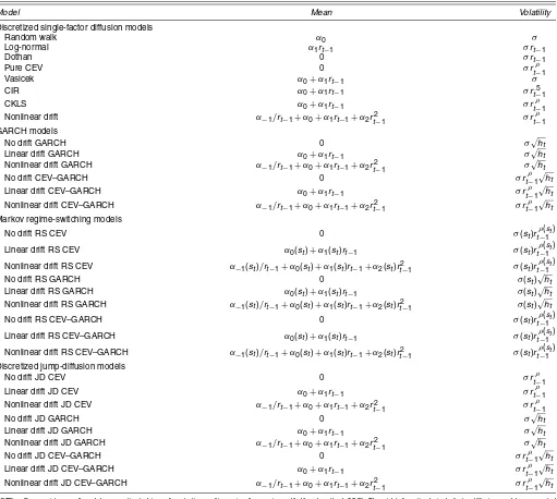
Table 1. Spot Rate Models Considered for Density Forecast Evaluation
NOTE: For consistency, all models are estimated in a discrete time setting using the maximum likelihood method (MLE). The eight discretized single-factor diffusion models are nested by the following specification: rt−1=α−1/rt−1+α0+α1rt−1+α2r2t−1+σr
we assume that the transition probability of{st}depends on the
once-lagged spot rate level,
Pr(st=l|st−1=l)=
1
1+exp(−cl−dlrt−1)
.
Table 1 lists a variety of regime-switching models, all of which are nested by the following specification:
As in the aforementioned models, we consider three specifica-tions of the conditional mean: zero, linear, and nonlinear drift. We also consider three specifications of the conditional vari-ance: CEV, GARCH, and combined CEV–GARCH. Thus we have a total of nine regime-switching models.
Although Gray (1996) removed the path-dependent nature of GARCH models by averaging the conditional and un-conditional variances over regimes at every time point, we use the same GARCH specification across different regimes. Confirming results of Ang and Bekaert (2002), we find a very unstable estimation of Gray’s (1996) model. In contrast, our specification turns out to have much better convergence prop-erties. Unlike many previous studies that set the elasticity parameter equal to .5, we allow it to be regime-dependent and
estimate it from the data. For identification, we set the diffusion constantσ (st)=1 for st=1 in the regime-switching models
with GARCH effect.
The conditional density of the interest rate rt in a
regime-switching model is
where the ex ante probability that the data are generated from regimelatt, Pr(st=l|It−1), can be obtained using Bayes’s rule
via a recursive procedure described by Hamilton (1989). The conditional density of regime-switching models is a mixture of two normal distributions, which can generate unimodal or bi-modal distributions and allows for great flexibility in modeling skewness, kurtosis, and heavy tails.
3.4 Jump-Diffusion Models
There are compelling economic and statistical reasons to account for discontinuity in interest rate dynamics. Various eco-nomic shocks, news announcements, and government interven-tions in bond markets have pronounced effects on the behavior of interest rates and tend to generate large jumps in interest rate data. Statistically, Das (2002) and Johannes (2003), among others, have shown that diffusion models (even with stochastic volatility) cannot generate the excessive leptokurtosis exhibited by the changes of the spot rates and that jump-diffusion mod-els are a convenient way to generate excessive kurtosis or, more generally, heavy tails.
We consider a class of discretized jump-diffusion mod-els listed Table 1. As in the aforementioned modmod-els, we consider zero, linear, and nonlinear drift specifications and CEV, GARCH and combined CEV–GARCH specifications for volatility. The nine different jump-diffusion models are nested by the following specification:
whereJ is the jump size andqt is the jump probability with
qt=1+exp(−1c−dr
t−1).
The conditional density of the foregoing jump-diffusion models can be written as
f(rt|rt−1)
ance of the diffusion part in (4). Similar to the regime-switching models, the conditional density of the jump-diffusion mod-els is also a mixture of two normal distributions. Thus these two classes of models represent two alternative approaches to generating excess kurtosis and heavy tails, although the regime-switching models have more sophisticated specifica-tions. For example, in (3) all drift parameters are regime-dependent, whereas in (4) only the intercept term is different in the conditional mean and variance. For the regime-switching models in (3), the state probabilities evolve according to a tran-sition matrix with updated priors at every time point. Thus it can capture both very persistent and transient regime shifts. For the jump-diffusion models in (4), the state probabilities are as-sumed to depend on the past interest rate level.
The in-sample performances of the four classes of models that we study have been individually studied in the literature. However, no one has yet attempted a systematic evaluation of all of these models in a unified setup, particularly in the out-of-sample context, because of the difficulty in density forecast evaluation and because of different nonnested specifications between existing classes of models. In the next section we com-pare the relative performance of these four classes of models in out-of-sample density forecast using the evaluation method described in Section 2. This comparison can provide valuable information about the relative strengths and weaknesses of each model and should be important for many applications.
4. MODEL ESTIMATION AND IN–SAMPLE PERFORMANCE
4.1 Data and Estimation Method
In modeling spot interest rate dynamics, yields on short-term debts are often used as proxies for the unobservable instan-taneous risk-free rate. These include the 1-month T-bill rates used by Gray (1996) and Chan, Karolyi, Longstaff, and Sanders (CKLS) (1992), the 3-month T-bill rates used by Stanton (1997) and Andersen and Lund (1997), the 7-day Eurodollar rates used by Ait-Sahalia (1996) and Hong and Li (2004), and the Fed funds rates used by Conley, Hansen, Luttmer, and Scheinkman (1997) and Das (2002). In our study, we follow CKLS (1992) and use the daily 1-month T-bill rates from June 14, 1961 to De-cember 29, 2000, with a total of 9,868 observations. The data are extracted from the CRSP bond file using the midpoint of quoted bid and ask prices of the T-bills with a remaining ma-turity that is closest to 1 month (30 calendar days) from the current date. Most of these T-bills have maturities of 6 months or 1 year when first issued and all T-bills used in our study have a remaining maturity between 27 and 33 days. We then com-pute the annualized continuously compounded yield based on the average of the ask and bid prices.
Figure 1 plots the level and change series of the daily 1-month T-bill rates, as well as their histograms. There is obvious persistent volatility clustering, and in general, the volatility is higher at a higher level of the interest rate (e.g., the 1979–1982 period). The marginal distribution of the inter-est rate level is skewed to the right, with a long right tail. Most daily changes in the interest rate level are very small, giving a
Figure 1. Daily 1-Month T-Bill Rates Between June 14, 1961 and December 29, 2000. This figure plots the level and change series of the daily 1-month T-bill rates, as well as their histograms. The data are extracted from the CRSP bond file using the midpoint of quoted bid and ask prices of the T-bills with a remaining maturity that is closest to 1 month (30 calendar days) from the current date.
sharp probability peak around 0. Daily changes of other spot in-terest rates, such as 3-month T-bill and 7-day Eurodollar rates, also exhibit a high peak around 0. But the peak is much less pronounced for weekly changes in spot rates. This, together with the long (right) tail, implies excess kurtosis, a stylized fact that has motivated the use of jump models in the literature (e.g., Das 2002; Johannes 2003).
We divide our data into two subsamples. The first, from June 14, 1961 to February 22, 1991 (with a total of 7,400 ob-servations), is a sample used to estimate model parameters; the second, from February 23, 1991 to December 29, 2000 (with a total of 2,467 observations), is a prediction sample used to evaluate out-of-sample density forecasts. We first consider the in-sample performance of the various models listed in Table 1, all of which are estimated using the MLE method. The opti-mization algorithm is the well-known BHHH with STEPBT for step length calculation and is implemented via the constrained optimization code in GAUSS Windows Version 5.0. The op-timization tolerance level is set such that the gradients of the parameters are less than or equal to 10−6.
Tables 2–5 report parameter estimates of four classes of spot rate models using daily 1-month T-bill rates from June 14, 1961 to February 22, 1991, with a total of 7,400 observations. To ac-count for the special period between October 1979 and Septem-ber 1982, we introduce dummy variables to the drift, volatility, and elasticity parameters; that is,αD,σD, andρD equal 0
out-side of the 1979–1982 period. We also introduce a dummy variable,D87, in the interest rate level to account for the effect
of 1987 stock market crash.D87 equals 0 except for the week
right after the stock market crash. Estimated robust standard er-rors are reported in parentheses.
4.2 In-Sample Evidence
We first discuss the in-sample performance of models within each class and then compare their performance across dif-ferent classes. Many previous studies (e.g., Bliss and Smith
1998) have shown that the period between October 1979 and September 1982, which coincides with the Federal Reserve ex-periment, has a big impact on model parameter estimates. To account for the special feature of this period, we introduce dummy variables in the drift, volatility, and elasticity parame-ters for this period. We also introduce a dummy variable in the interest rate level for the week right after 1987 stock market crash. Brenner et al. (1996) showed that the decline of the in-terest rates during this week is too dramatic to be captured by most standard models.
Table 2 reports parameter estimates with estimated robust standard errors and log-likelihood values for discretized single-factor diffusion models. The estimates of the drift parameters of Vasicek, CIR, and CKLS models all suggest mean-reversion in the conditional mean, with an estimated 6% long-run mean. For other models, such as the random walk, log-normal, and nonlinear drift models, most drift parameters are not signifi-cant. A comparison of the pure CEV, CKLS, and Ait-Sahalia (1996) nonlinear drift models indicates that the incremental contribution of nonlinear drift is very marginal, which is not surprising given that the drift parameter estimates in the non-linear drift model are mostly insignificant. On the other hand, there is also a clear evidence of level effect; all estimates of the elasticity parameter are significant. Unlike previous stud-ies (e.g., CKLS 1992), which found an estimated elasticity pa-rameter close to 1.5, our estimate is about .25 (.70) outside (inside) the 1979–1982 period. Our results confirm previous findings of Brenner et al. (1996), Andersen and Lund (1997), Bliss and Smith (1998), and Koedijk, Nissen, Schotman, and Wolff (1997) that the estimate of the elasticity parameter is very sensitive to the choice of interest rate data, data frequency, sample periods, and specifications of the volatility function. The 1979–1982 period dummies suggest that the drift does not behave very differently (i.e., αD is not significant), whereas
volatility is significantly higher and depends more heavily on
Table 2. Parameter Estimates for the Single-Factor Diffusion Models
Nonlinear Parameters RW Log-normal Dothan Pure CEV Vasicek CIR CKLS drift
α−1 .0289
(.0751)
α0 .0012 .0196 .0190 .0199 −.0098
(.0019) (.0056) (.0049) (.0053) (.0485)
α1 .0006 −.0033 −.0032 −.0034 .0045
(.0004) (.0010) (.0009) (.0009) (.0095)
α2 −.0006
(.0006)
σ .1523 .0304 .0304 .1011 .1522 .0658 .1007 .1007
(.0013) (.0003) (.0003) (.0041) (.0013) (.0006) (.0041) (.0041)
ρ .2437 .2460 .2460
(.0238) (.0238) (.0238)
αD −.0047 .0196 .0154 .0233 .0266 .0402
(.0157) (.0186) (.0168) (.0176) (.0168) (.0202)
σD .2768 .0175 .0175 .2764 .0712
(.0112) (.0013) (.0013) (.0112) (.0036)
ρD .3692 .3684 .3680
(.0132) (.0132) (.0132)
D87 −.3988 −.2107 −.2079 −.3549 −.4003 −.3101 −.3574 −.3582 (.0681) (.0660) (.0660) (.0671) (.0681) (.0655) (.0670) (.0671) Log-likelihood 2,649.6 2,187.0 2,184.9 2,654.5 2,655.5 2,672.0 2,661.7 2,662.5
NOTE: The models are nested by the following specification:rt=α−1/rt−1+(α0+αD)+α1rt−1+α2rt2−1+(σ+σD)rt(ρ−+1ρD)zt+D87, where
{zt}∼iid N(0, 1).
the interest rate level in this period (i.e.,σDandρD are
signif-icantly positive) than in other periods. For models with level effect, we introduce the dummy only for elasticity parameterρ, to avoid the offsetting effect of dummies in ρ andσ, which would tend to generate unstable estimates. The stock market crash dummy is significantly negative, which is consistent with the findings of Brenner et al. (1996).
Estimation results of GARCH models in Table 3 show that GARCH significantly improves the in-sample fit of dif-fusion models (i.e., the log-likelihood value increases from
about 2,500 to about 5,700). Previous studies, such as those by Bali (2001) and Durham (2003), have also shown that for single-factor diffusion, GARCH, and continuous-time stochas-tic volatility models, it is more important to correctly model the diffusion function than the drift function in fitting interest rate data. This suggests that volatility clustering is an important feature of interest rates. All estimates of GARCH parameters are overwhelmingly significant. The sum of GARCH parame-ter estimates,βˆ1+ ˆβ2, is slightly larger (smaller) than 1 without
(with) level effect. Although the sum of GARCH parameters is
Table 3. Parameter Estimates for the GARCH Models
No drift Linear drift Nonlinear drift No drift Linear drift Nonlinear drift Parameters GARCH GARCH GARCH CEV–GARCH CEV–GARCH CEV–GARCH
α−1 .1556 .1716
(.0470) (.0457)
α0 .0053 −.1117 .0063 −.1233
(.0025) (.0323) (.0025) (.0311)
α1 −.0003 .0263 −.0006 .0290
(.0006) (.0069) (.0006) (.0066)
α2 −.0018 −.0020
(.0004) (.0004)
ρ .1709 .1797 .1926
(.0298) (.0301) (.0300)
β0 9.7E−05 8.6E−05 8.6E−05 8.9E−05 8.2E−05 8.2E−05
(1.2E−05) (1.2E−05) (1.6E−05) (1.0E−05) (.9E−05) (.9E−05)
β1 .1552 .1544 .1563 .0896 .0875 .0851
(.0097) (.0096) (.0099) (.0104) (.0101) (.0098)
β2 .8707 .8723 .8712 .8583 .8582 .8553
(.0065) (.0064) (.0065) (.0074) (.0076) (.0078)
αD .0166 .1119 .0550 .1317
(.0318) (.0229) (.0282) (.0201)
σD .1368 .1302 .1017
(.0327) (.0331) (.0334)
ρD .0151 .0064 −.0053
(.0134) (.0146) (.0142)
D87 −.5397 −.5426 −.5460 −.5288 −.5318 −.5352
(.0774) (.0777) (.0771) (.0753) (.0751) (.0741) Log-likelihood 5,686.8 5,699.5 5,706.3 5,701.1 5,715.2 5,725.5
NOTE: The models are nested by the following specification:rt=α−1/rt−1+(α0+αD)+α1rt−1+α2rt2−1+(1+σD)rt(ρ−+1ρD)
√
htzt+D87, where
ht=β0+ht−1(β2+β1rt2−ρ1zt2−1) and {zt}∼iid N(0, 1).
Table 4. Parameter Estimates for the Markov Regime-Switching Models
Linear drift Nonlinear drift No drift Linear drift Nonlinear drift No drift Linear drift Nonlinear drift Parameters No drift CEV CEV CEV GARCH GARCH GARCH CEV–GARCH CEV–GARCH CEV–GARCH
α−1(1) .0607 .3321 .2646
(.3569) (.1701) (.1605)
α0(1) .0973 .1517 .0457 −.1462 .0450 −.1086
(.0259) (.2027) (.0107) (.1009) (.0105) (.0989)
α1(1) −.0102 −.0288 −.0043 .0274 −.0042 .0209
(.0031) (.0321) (.0019) (.0181) (.0019) (.0185)
α2(1) .0011 −.0015 −.0011
(.0014) (.0010) (.0011)
σ(1) .3361 .3171 .3106 1 1 1 1 1 1
(.0302) (.0287) (.0281)
ρ(1) .1021 .1277 .138 0 0 0 .1193 .1589 .1670
(.044) (.0446) (.0448) (.0452) (.0460) (.0487)
α−1(2) −.0352 −.0267 −.0286
(.0329) (.0242) (.0183)
α0(2) −.0002 .0141 −.0013 .0062 −.0020 .0062
(.0020) (.0229) (.0017) (.0153) (.0018) (.0104)
α1(2) −.0006 −.0012 −.0008 −.0001 −.0007 .0005
(.0004) (.0048) (.0004) (.0031) (.0004) (.0020)
α2(2) −.0001 −.0002 −.0002
(.0003) (.0002) (.0001)
σ(2) .0143 .0141 .0138 .2566 .2567 .2574 .2769 .3034 .3051
(.0010) (.0010) (.0010) (.006) (.006) (.006) (.0275) (.0303) (.0311)
ρ(2) .8122 .8179 .8257 0 0 0 .0844 .0727 .0800
(.0403) (.0422) (.0421) (.0602) (.0602) (.0611)
β0 3.83E−4 3.18E−4 2.96E−4 3.21E−4 2.43E−4 2.25E−4
(7.11E−5) (6.14E−5) (5.79E−5) (.67E−4) (.50E−4) (.47E−4)
β1 .0357 .0336 .0335 .0265 .0259 .0252
(.004) (.0039) (.0038) (.0057) (.0055) (.0053)
β2 .9027 .9066 .9077 .8972 .8993 .9001
(.009) (.0089) (.0086) (.0099) (.0098) (.0094)
c1 .3132 .3001 .3171 −1.2515 −1.2007 −1.1293 −1.1954 −1.1429 −1.0012
(.2734) (.273) (.2683) (.3211) (.3065) (.3136) (.3819) (.3705) (.3674)
d1 .1081 .107 .1029 .1303 .1295 .1192 .1190 .1193 .0959
(.0391) (.039) (.0381) (.044) (.0426) (.0447) (.0594) (.0582) (.0593)
c2 4.0963 4.0342 4.0089 1.8864 1.7868 1.7633 1.8227 1.7299 1.6947
(.2386) (.2393) (.2313) (.2048) (.1947) (.1909) (.2092) (.1983) (.2009)
d2 −.2302 −.225 −.2225 −.0938 −.0806 −.0776 −.0906 −.0810 −.0757
(.0354) (.0354) (.0339) (.0276) (.0263) (.0257) (.0285) (.0276) (.0283) Log-likelihood 6,493.1 6,507.9 6,512.8 7,079.0 7,132.8 7,138.2 7,082.8 7,138.6 7,144.1
NOTE: The models are nested by the following specification:rt=α−1(st)/rt−1+α0(st)+α1(st)rt−1+α2(st)rt2−1+σ(st)rρt−(st1)
√
htzt, whereht=β0+β1E{et|rt−2,st−2}2+β2ht−1,
et= [rt−1−E(rt−1|rt−2,st−1)]/σ(st−1), {zt}∼iid N(0, 1), andstfollows a two-state Markov chain with transition probability Pr (st=l|st−1=l)=(1+exp (−cl−dlrt−1))−1forl=1, 2.
slightly larger than 1, it is still possible that the spot rate model is strictly stationary (see Nelson 1991 for more discussion). We also find a significant level effect even in the presence of GARCH, but the estimated elasticity parameter is close to .20, which is much smaller than that of single-factor diffusion mod-els. The specification of conditional variance also affects the es-timation of drift parameters. Unlike those in diffusion models, most drift parameter estimates in linear drift GARCH models are insignificant. Among all GARCH models considered, the one with nonlinear drift and level effect has the best in-sample performance. In the 1979–1982 period, the interest rate volatil-ity is significantly higher, but its dependence on the interest rate level is not significantly different from other periods. The 1987 stock market crash dummy is again significantly negative.
Parameter estimates of regime-switching models, given in Table 4, show that the spot rate behaves quite differently between two regimes. Although the sum of GARCH parame-ters is slightly larger than 1, it is still possible that the spot rate model is strictly stationary (see Nelson 1991 for more discus-sion). For models with a linear drift, in the first regime the spot rate has a high long-run mean (about 10%) and exhibits strong
mean reversion (i.e., estimates of the mean-reversion speed pa-rameter are significantly negative). The spot rate in the second regime behaves almost like a random walk, because most drift parameter estimates are close to 0 and insignificant. For mod-els with a nonlinear drift, all drift parameters are insignificant. Volatility in the first regime is much higher, about three times that in the second regime. Our estimates show that level ef-fect, although significant in both regimes, is much stronger in the second regime in the absence of GARCH. After including GARCH, the elasticity parameter estimate becomes insignif-icant in the second regime, but remains the same in the first regime. Apparently, regime switching helps capture volatility clustering; the sum of GARCH parameters,βˆ1+ ˆβ2, is smaller
in regime-switching models than in pure GARCH models. The estimated transition probabilities of the Markov state variablest
show that the low-volatility regime is much more persistent than the high-volatility regime. Our results suggest that the spot rate evolves like a random walk with low volatility most of time, oc-casionally increasing and evolving with strong mean reversion and high volatility. Overall, the regime-switching model with a linear drift in each regime, CEV, and GARCH has the best in-sample performance.
Table 5. Parameter Estimates for the Jump-Diffusion Models
Linear drift Nonlinear drift No drift Linear drift Nonlinear drift No drift Linear drift Nonlinear drift Parameters No drift CEV CEV CEV GARCH GARCH GARCH CEV–GARCH CEV–GARCH CEV–GARCH
α−1 .0264 .0702 .0661
(.0293) (.0384) (.0380)
α0 −.0011 −.0340 .0028 −.0506 .0026 −.0486
(.0169) (.0203) (.0019) (.0256) (.0020) (.0253)
α1 −.0007 .0101 −.0013 .0110 −.0012 .0107
(.0004) (.0043) (.0004) (.0053) (.0004) (.0052)
α2 −.0009 −.0008 −.0008
(.0003) (.0003) (.0003)
σ .0127 .0126 .0124
(.0008) (.0008) (.0008)
ρ .8936 .8975 .9045 .0929 .0852 .0837
(.0390) (.0397) (.0400) (.0518) (.0510) (.0512)
β0 8.7E−05 8.8E−05 8.7E−05 7.6E−5 7.7E−5 7.7E−5
(1.2E−05) (1.2E−05) (1.2E−05) (1.2E−5) (1.2E−5) (1.2E−5)
β1 .0631 .0640 .0635 .0450 .0472 .0472
(.0076) (.0073) (.0073) (.0101) (.0102) (.0102)
β2 .8514 .8484 .8499 .8504 .8471 .8483
(.0139) (.0134) (.0134) (.0140) (.0135) (.0134)
c −2.7404 −2.7057 −2.6972 −3.7908 −3.7470 −3.7481 −3.6908 −3.6498 −3.6518 (.1608) (.1605) (.1614) (.1982) (.1970) (.1976) (.2097) (.2084) (.2093)
d .1451 .1423 .1397 .2554 .2516 .2509 .2293 .2274 .2272
(.0275) (.0275) (.0275) (.0307) (.0305) (.0307) (.0343) (.0340) (.0341)
µ .0233 .0385 .0321 .0700 .0887 .0895 .0679 .0892 .0897
(.0133) (.0142) (.0128) (.0152) (.0158) (.0158) (.0162) (.0164) (.0163)
γ .4316 .4279 .4304 .3928 .3903 .3929 .4109 .4046 .4061
(.0117) (.0120) (.0104) (.0197) (.0189) (.0187) (.0199) (.0182) (.0178)
αD −.0094 .0296 −.0192 .0057 −.0197 .0055
(.0121) (.0112) (.0117) (.0154) (.0112) (.0150)
σD −.1027 −.1328 −.1551
(.1142) (.1054) (.1033)
ρD .1473 .1872 −.0697 −.1220 −.1186 −.1277
(.1079) (.0703) (.0722) (.0769) (.0573) (.0564)
cD 4.1604 4.3364 4.0036 4.0290 4.2505 4.1857 3.8622 4.0677 4.0272
(.6523) (.6535) (.5477) (.7495) (.7546) .7421 (.6911) (.7129) (.7019)
dD −.2441 −.2721 −.1836 −.2748 −.2860 −.2791 −.2320 −.2487 −.2445
(.0808) (.0730) (.0534) (.0689) (.0682) .0667 (.0685) (.0676) (.0662)
D87 −.4283 −.4253 −.4266 −.4226 −.4198 −.4217 −.4233 −.4209 −.4225
(.0646) (.0641) (.0643) (.0826) (.0820) (.0815) (.0793) (.0793) (.0791) Log-likelihood 6,306.3 6,317.2 6,326.3 6,794.1 6,810.8 6,813.9 6,796.3 6,812.9 6,816.1
NOTE: The models are nested by the following specification:rt=α−1/rt−1+(α0+αD)+α1rt−1+α2rt2−1+(σ+σD)rt(ρ−+1ρD)
√
htzt+J(µ,γ2)πt(qt+qD)+D87, whereht=β0+
β1[rt−1−E(rt−1|rt−2)]2+β2ht−1, {zt}∼iid N(0, 1),J∼N(µ,γ2), andπt(qt+qD) is Bernoulli(qt+qD) withqt+qD=(1+exp (−c−cD−(d+dD)·rt−1))−1.
Table 5 reports parameter estimates for discretized jump-diffusion models. There is some weak evidence of mean re-version, especially when there is GARCH. The contribution of nonlinear drift is again very marginal: most estimated drift pa-rameters are insignificant. For jump-diffusion models, without GARCH, the elasticity parameter estimate is about .9, which is closer to the 1.5 found by CKLS. However, level effect is weakened (i.e., ρˆ becomes close to .1) after GARCH is in-troduced. It seems that CEV helps capture part of volatility clustering, but its importance diminishes in the presence of GARCH. We find that GARCH also significantly improves the performance of jump-diffusion models. Without GARCH, there is a high probability of small jumps, with an estimated mean jump size between 2% and 4%. With GARCH, the jump probability becomes smaller, but the mean jump size increases to about between 7% and 9%. This suggests that without GARCH, jumps can capture part of volatility clustering, but with GARCH, jumps mainly capture large interest rate move-ments. Of course, jumps also help explain volatility cluster-ing; the sum of GARCH parameters is again much smaller than that in pure GARCH models. During the 1979–1982 pe-riod, other than the probability of jumps becoming
substan-tially higher, other aspects of the jump-diffusion models (e.g., the drift, volatility, or elasticity parameter) do not behave very differently.
To sum up, our in-sample analysis reveals some important stylized facts for the spot rate:
1. The importance of modeling mean reversion in mean is ambiguous. It seems that linear drift is adequate for this purpose once GARCH, regime switching, or jumps are included. The contribution of Ait-Sahalia’s (1996) type of nonlinear drift is very marginal.
2. It is important to model conditional heteroscedasticity through GARCH or level effect, although GARCH seems to have much better in-sample performance than CEV. 3. Regime switching and jumps help capture volatility
clus-tering and especially the excess kurtosis and heavy-tails of the interest rate.
4. Interest rates behave quite differently during the 1979–1982 period. The level and volatility of the inter-est rate, the dependence of the interinter-est rate volatility on the interest rate level, and the probability of jumps are much higher during this period.
5. OUT–OF–SAMPLE DENSITY FORECAST PERFORMANCE
The foregoing in-sample analysis demonstrates that model-ing volatility clustermodel-ing through GARCH and heavy tails and excess kurtosis through regime switching or jumps significantly improves the in-sample fit of historical interest rate data. How-ever, it is not clear whether these models will also perform well in out-of-sample density forecasts for future interest rates. Indeed, some previous studies have shown that more compli-cated models actually underperform the simple random walk model in predicting the conditional mean of future interest rates (e.g., Duffee 2002). In many financial applications, we are interested in forecasting the whole conditional distribu-tion. We now apply the generalized spectral evaluation method described in Section 2 to evaluate density forecasts of the mod-els under study. Among other things, we examine whether the features found to be important for in-sample performance remain important for out-of-sample forecasts, and whether the best in-sample performing models still perform best in out-of-sample forecasts.
For each model, we first calculate{Zt(θ )ˆ }, then model
gen-eralized residuals using the prediction sample, with model parameter estimates based on the estimation sample. Table 6 reports the out-of-sample evaluation statistic M1 for each
model. To computeM1, we select a normal cdf(
√
12u)for the weighting functionW(u)and a Bartlett kernel for the kernel functionk(z). To choose a lag order p, we use a data-driven method that minimizes the asymptotic integrated mean squared error of the modified generalized spectral density. This method involves choosing a preliminary lag orderp¯.We examine a wide range ofp¯ in our application. We obtain similar results for the preliminary lag orderp¯between 10 and 30 and report results for
¯
p=20 in Table 6. For comparison, we also report the in-sample log-likelihood values obtained from the estimation sample.
TheM1 statistics show that all single-factor diffusion
mod-els are overwhelmingly rejected. One of the most interesting findings is that models that include a drift term (either linear or nonlinear) have much worse out-of-sample performance than those without a drift. Dothan’s (1978) model and the pure CEV model have the best density forecast performance. Both mod-els have a zero drift and level effect, the elasticity parameter ρ=1 for the former and .25 (.60 for the 1979–1982 period) for the latter. On the other hand, although the CKLS model and Ait-Sahalia’s (1996) nonlinear drift model have the highest in-sample likelihood values, they have the worst out-of-sample density forecasts in terms ofM1. This seems to suggest that for
the purpose of density forecast, it is much more important to model the diffusion function than the drift function. Of course, this does not necessarily mean that the drift is not important.
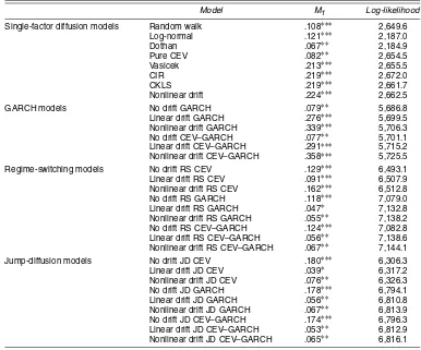
Table 6. Out-of-Sample Density Forecast Performance of Spot Interest Rate Models
Model M1 Log-likelihood
Single-factor diffusion models Random walk .108∗∗∗ 2,649.6
Log-normal .121∗∗∗ 2,187.0
Dothan .067∗∗ 2,184.9
Pure CEV .082∗∗ 2,654.5
Vasicek .213∗∗∗ 2,655.5
CIR .219∗∗∗ 2,672.0
CKLS .219∗∗∗ 2,661.7
Nonlinear drift .224∗∗∗ 2,662.5
GARCH models No drift GARCH .079∗∗ 5,686.8
Linear drift GARCH .276∗∗∗ 5,699.5 Nonlinear drift GARCH .339∗∗∗ 5,706.3
No drift CEV–GARCH .077∗∗ 5,701.1
Linear drift CEV–GARCH .291∗∗∗ 5,715.2 Nonlinear drift CEV–GARCH .358∗∗∗ 5,725.5 Regime-switching models No drift RS CEV .129∗∗∗ 6,493.1 Linear drift RS CEV .091∗∗∗ 6,507.9 Nonlinear drift RS CEV .162∗∗∗ 6,512.8
No drift RS GARCH .118∗∗∗ 7,079.0
Linear drift RS GARCH .047∗ 7,132.8 Nonlinear drift RS GARCH .055∗∗ 7,138.2 No drift RS CEV–GARCH .124∗∗∗ 7,082.8 Linear drift RS CEV–GARCH .056∗∗ 7,138.6 Nonlinear drift RS CEV–GARCH .067∗∗ 7,144.1 Jump-diffusion models No drift JD CEV .180∗∗∗ 6,306.3
Linear drift JD CEV .039∗ 6,317.2
Nonlinear drift JD CEV .076∗∗ 6,326.3
No drift JD GARCH .178∗∗∗ 6,794.1
Linear drift JD GARCH .056∗∗ 6,810.8 Nonlinear drift JD GARCH .067∗∗ 6,813.9 No drift JD CEV–GARCH .174∗∗∗ 6,796.3 Linear drift JD CEV–GARCH .053∗∗ 6,812.9 Nonlinear drift JD CEV–GARCH .065∗∗ 6,816.1
NOTE: This table reports the out-of-sample density forecast performance of the single-factor diffusion, GARCH, Markov regime-switching, and jump-diffusion models measured by theM1statistic. For convenience of comparison, we also report the in-sample log-likelihood value for each
model. The in-sample parameter estimation is based on the observations from June 14, 1961 to February 2, 1991, and the out-of-sample density forecast evaluation is based on the observations from February 23, 1991 to December 29, 2000. The ratio between the size of the estimation sample and the forecast sample is about 3 : 1. In computing the out-of-sampleM1statistics, a preliminary lag orderp¯of 20 is used. Other lag
orders give similar results. The asymptotic critical values for the out-of-sample evaluation statistic are .087, .051, and .037 at the 1%, 5%, and 10% levels and∗∗∗,∗∗, and∗indicate that theM1statistic is significant at the 1%, 5%, and 10% levels.
It might be simply because the drift specifications considered are severely misspecified and do not outperform the zero drift model. In fact, most drift parameter estimates have large stan-dard errors and thus have excess sampling variation in para-meter estimation. As a consequence, assuming zero drift may result in a smaller adverse effect on out-of-sample performance. The generalized residuals{Zt(θ )ˆ }contain much information
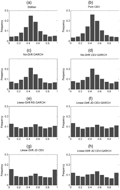
about possible sources of model misspecification. Instead of being uniform, the histograms of the generalized residuals for all diffusion models (Fig. 2) exhibit a high peak in the cen-ter of the distribution, which indicates that the diffusion mod-els cannot satisfactorily capture the marginal density of the spot rate. The separate inference statistics M(m,l)in Table 7 also show that all the models fail to satisfactorily capture the dynamics of the generalized residuals. In particular, the large
M(2,2) and M(4,4) statistics indicate that diffusion models perform rather poorly in modeling the conditional variance and kurtosis of the generalized residuals.
Similar to single-factor diffusion models, GARCH models with a zero drift have much better density forecasts than those models with a linear or nonlinear drift. The best GARCH and diffusion models haveM1 statistics roughly between .07
(a) (b)
(c) (d)
(e) (f)
(g) (h)
Figure 2. Histograms of the Generalized Residuals of Four Classes of Spot Rate Models. This figure plots the histograms of the generalized residuals of the single-factor diffusion, GARCH, regime-switching, and jump-diffusion spot rate models.
and .08. Comparing the best GARCH and single-factor dif-fusion models, we find that GARCH provides better density forecasts than CEV, and combining CEV and GARCH further improves the density forecasts. Diagnostic analysis of general-ized residuals shows that GARCH models provide certain im-provements over diffusion models. For example, the histograms of the generalized residuals of GARCH models have a less-pronounced peak in the center. TheM(m,l)statistics show that GARCH models significantly improve the fitting of even-order moments of the generalized residuals; theM(2,2)andM(4,4) statistics are reduced from close to 100 to single digits!
In summary, our analysis of single-factor diffusion and GARCH models demonstrates that both classes of models fail to provide good density forecasts for future interest rates. They fail to capture both the high peak in the center of the mar-ginal density and the dynamics of different moments of the generalized residuals. GARCH models have a more uniform marginal density and significantly improve the ability to model the dynamics of even-order moments of the generalized residu-als. For both classes of models, modeling the conditional vari-ance through CEV or GARCH is much more important than modeling the conditional mean of the interest rate. Zero-drift models outperform either linear or nonlinear drift models in density forecast, although the M(1,1) statistics suggest that neither model adequately captures the dynamic structure in the conditional mean of the generalized residuals.
We next turn to regime-switching models. Regime-switching models generally have better density forecasts than single-factor diffusion and GARCH models: the best regime-switching models reduce the M1 statistics of the best diffusion and
GARCH models from above .07 to about .05. Although mod-eling the drift does not improve density forecast for diffusion and GARCH models, the best regime-switching models in den-sity forecast have a linear drift in each regime. As pointed out by Ang and Bekaert (2002) and Li and Xu (2000), a regime-switching model with a linear drift in each regime actually im-plies nonlinear conditional mean dynamics for the interest rate. Thus our results suggest that perhaps a specific nonlinear drift is needed for out-of-sample density forecasts. GARCH is more important than CEV for density forecasts, and combining CEV with GARCH does not further improve model performance. Overall, the regime-switching GARCH model with a linear drift in each regime provides the best out-of-sample forecasts among all of the regime-switching models. Diagnostic analysis shows that regime-switching models provide a much better charac-terization of the marginal density of interest rates; the his-tograms of the generalized residuals are much closer to U[0,1]. TheM(2,2)andM(4,4)statistics of regime-switching models are slightly higher than those of GARCH models, however, and theM(1,1)andM(3,3)statistics of regime-switching models are actually higher than those of diffusion and GARCH models. Therefore the advantages of regime-switching models seem to come from better modeling of the marginal density, rather than from the dynamics of the generalized residuals.
The density forecast performance of jump-diffusion models shares many common features with that of regime-switching models. First, they have comparable performance; theM1
sta-tistics of the best jump-diffusion models are also around .05. Second, for jump-diffusion models, the linear drift
Table 7. Separate Inference Statistics for Out-of-Sample Density Forecast Performance
Model M(1, 1) M(1, 2) M(2, 1) M(2, 2) M(3, 3) M(4, 4)
Single-factor diffusion models
Random walk 40.08 6.35 40.48 99.73 21.50 80.12
Log-normal 46.52 8.77 39.91 110.10 26.98 92.51
Dothan 46.04 8.07 42.62 108.90 27.02 91.03
Pure CEV 41.62 6.63 41.55 96.81 22.85 80.42
Vasicek 40.40 8.13 35.55 100.20 21.43 81.79
CIR 43.61 8.68 36.30 98.57 24.39 85.02
CKLS 42.02 8.55 35.75 97.89 22.80 82.77
Nonlinear drift 42.40 8.37 35.93 98.47 22.77 82.98
GARCH models
No drift GARCH 40.73 3.75 28.21 7.68 17.57 2.53
Linear drift GARCH 41.07 4.66 25.11 7.53 17.00 2.35
Nonlinear drift GARCH 40.71 4.87 24.70 7.02 16.63 2.09
No drift CEV–GARCH 41.30 4.10 28.40 7.46 19.24 2.74
Linear drift CEV–GARCH 41.68 5.11 25.06 7.09 18.73 2.44
Nonlinear drift CEV–GARCH 41.43 5.45 24.32 6.45 18.54 2.17
Regime-switching models
No drift RS CEV 53.16 3.13 11.31 7.05 35.02 10.21
Linear drift RS CEV 53.25 4.56 11.16 6.57 34.31 8.83
Nonlinear drift RS CEV 53.75 5.12 9.84 6.56 34.50 8.49
No drift RS GARCH 57.29 4.05 21.59 10.95 43.71 7.63
Linear drift RS GARCH 55.46 4.56 21.09 12.38 40.71 9.14
Nonlinear drift RS GARCH 55.69 4.50 21.05 12.14 41.13 8.93
No drift RS CEV–GARCH 45.35 3.69 20.91 10.67 34.25 7.08
Linear drift RS CEV–GARCH 44.10 4.86 20.75 11.99 32.12 8.87 Nonlinear drift RS CEV–GARCH 44.36 4.84 20.55 11.40 32.46 8.32
Jump-diffusion models
No drift JD CEV 47.38 5.32 16.76 85.10 43.01 99.31
Linear drift JD CEV 46.32 4.48 19.63 85.09 42.26 99.82
Nonlinear drift JD CEV 46.50 4.85 18.31 85.10 42.48 99.29
No drift JD GARCH 43.32 5.10 20.35 12.38 28.44 8.96
Linear drift JD GARCH 42.57 4.60 21.48 12.19 28.22 8.84
Nonlinear drift JD GARCH 42.62 4.67 21.42 12.34 28.24 8.95
No drift JD CEV–GARCH 43.55 5.05 20.51 13.36 29.31 10.07
Linear drift JD CEV–GARCH 42.74 4.54 21.69 13.00 28.93 9.76 Nonlinear drift JD CEV–GARCH 42.78 4.62 21.57 13.07 28.94 9.81
NOTE: This table reports the separate inference statisticsM(m,l) for the four classes of spot rate models. The asymptotically normal statisticM(m,l) can be used to test whether the cross-correlation between themth andlth moments of {Zt} is significantly different from 0. The choice of (m,l)=(1, 1), (2, 2), (3, 3), and (4, 4) is sensitive to
autocorrelations in mean, variance, skewness, and kurtosis of {rt}. We report results only for a lag truncation orderp=20; the results forp=10 and 30 are rather similar. The
asymptotical critical values are 1.28, 1.65, and 2.33 at the 10%, 5%, and 1% levels.
cation outperforms those with no drift or nonlinear drift for density forecasts. Third, for jump-diffusion models, GARCH generally provides better density forecasts than CEV. Fourth, jump-diffusion models have similar advantages over single-factor diffusion and GARCH models. They have much bet-ter characbet-terization of the marginal density of the generalized residuals, but they may not necessarily perform better in mod-eling the dynamics of the generalized residuals, as indicated by their large M(m,l)statistics. The jump model with a lin-ear drift and level effect, although it has the smallestM1
statis-tic, apparently fails to capture the even-order moments of the generalized residuals, with M(2,2)andM(4,4)statistics sig-nificantly higher than other jump-diffusion models that include GARCH effects.
In summary, our out-of-sample density forecast evaluation reveals the following important features:
1. For out-of-sample density forecast, the importance of modeling mean reversion in the interest rate is ambiguous. For diffusion and GARCH models, a linear or nonlinear drift gives worse density forecasts than a zero drift. How-ever, when there are regime switches or jumps, linear drift models outperform those with zero or nonlinear drift. The best density forecast models still fail to adequately cap-ture the mean dynamics of the generalized residuals. 2. It is important to capture volatility clustering in interest
rates for both in-sample and out-of-sample performance
via GARCH. Most of the best-performing models have a GARCH component, which significantly improves their ability to model the dynamics of the even-order moments of the generalized residuals.
3. It is also important to capture excess kurtosis and heavy tails of the interest rate for both in-sample and out-of-sample performance via regime switching or jumps. The advantages of regime-switching and jump models are mainly reflected in modeling the marginal density, rather than in the dynamics of the generalized residuals.
Overall, our out-of-sample analysis demonstrates that more-complicated models that incorporate conditional heteroscedas-ticity and heavy tails of interest rates tend to have a better density forecast. This result is quite different from the results for those that focus on conditional mean forecast. As widely documented in the literature, the predictable component in the conditional mean of the interest rate appears insignificant. As a result, random walk models tend to outperform more-sophisticated models in terms of mean forecast (e.g., Duffee 2002). However, density forecast includes all conditional mo-ments, and as a result, those models that can capture the dy-namics of higher-order moments tend to have better density forecasts. Our analysis suggests that the more-complicated spot rate models developed in the literature can indeed capture some important features of interest rates and are relevant in applica-tions involving density forecasts of interest rates.
6. CONCLUSION
Despite the numerous empirical studies of spot interest rate models, little effort has been devoted to examining their out-of-sample forecast performance. We have contributed to the literature by providing the first (to our knowledge) compre-hensive empirical analysis of the out-of-sample performance of a wide variety of popular spot rate models in forecasting the conditional density of future interest rates. Out-of-sample density forecasts help minimize the data snooping bias due to excessive searching for more-complicated models using similar datasets. The conditional density, which completely character-izes the full dynamics of interest rates, is also an essential input to many financial applications. Using a rigorous econometric evaluation procedure for density forecasts, we examined the out-of-sample performance of single-factor diffusion, GARCH, regime-switching, and jump-diffusion models.
Although previous studies have shown that simpler models, such as the random walk model, tend to have more accurate forecasts for the conditional mean of interest rates, we find that models that capture conditional heteroscedasticity and heavy tails of the spot rate have better out-of-sample density forecasts. GARCH significantly improves modeling of the conditional variance and kurtosis of the generalized residuals, whereas regime-switching and jumps help in modeling the marginal density of interest rates. Therefore, our analysis shows that the more-sophisticated interest rate models developed in the litera-ture can indeed caplitera-ture some important fealitera-tures of interest rate data and perform better than simpler models in out-of-sample density forecasts. Although we have focused on density fore-casts of the spot rates here, there is evidence that the term struc-ture of interest rates is driven by multiple factors (e.g., Dai and Singleton 2000). Extending our analysis to forecast the joint density of multiple yields is an interesting issue that we will address in future research.
ACKNOWLEDGMENTS
The authors are grateful for the helpful comments of Canlin Li, Daniel Morillo, Larry Pohlman, and seminar participants at PanAgora Asset Management, the 2002 Econometric Society European Summer Meeting, and the 2003 Econometric Society North American Winter Meeting. They also thank the associate editor, and two anonymous referees, whose comments and sug-gestions have greatly improved the article, and David George for editorial assistance. Hong’s work was supported by National Science Foundation grant SES-0111769. Any errors are the au-thors’ own.
APPENDIX: GENERALIZED SPECTRAL EVALUATION FOR DENSITY FORECASTS
Here we describe Hong’s (2003) omnibus evaluation proce-dure for out-of-sample density forecasts, as well as a class of separate inference procedures. (For more discussion and formal treatment, see Hong 2003.)
A.1 Generalized Spectrum
Generalized spectrum was proposed by Hong (1999) as an analytic tool to provide an alternative to the power spectrum and the higher-order spectrum (e.g., bispectrum) in time series analysis. Define the centered generalized residual
Zt≡Zt(θ )=
characteristic function ϕ(u) ≡ E(eiuZt) and pairwise joint
characteristic function ϕj(u,v) ≡ E[exp{i(uZt + vZt−|j|)}],
wherei≡√−1,u,v∈(−∞,∞)andj=0,±1, . . . .The basic idea of generalized spectrum is to transform the series{Zt}and
then consider the spectrum of the transformed series. Define the generalized covariance function
σj(u,v)≡coveiuZt,eivZt−|j|, j=0,±1, . . . .
Straightforward algebra yields σj(u,v)=ϕj(u,v)−ϕ(u)ϕ(v).
Because ϕj(u,v) =ϕ(u)ϕ(v) for all (u,v) if and only if
Zt and Zt−|j| are independent (cf. Lukacs 1970), σj(u,v)can
capture any type of pairwise serial dependence in {Zt} over
various lags, including those with zero autocorrelation in{Zt}.
Under certain regularity conditions on the temporal depen-dence of{Zt}, the Fourier transform of the generalized
covari-ance functionσj(u,v)exists and is given by
rial dependence in {Zt} across various lags. An advantage of
spectral analysis is thatf(ω,u,v)incorporates all lags simulta-neously. Thus it can capture the dependent processes in which serial dependence occurs only at higher-order lags. This can arise from seasonality (e.g., calender effects) or time delay in financial markets. Moreover,f(ω,u,v)is particularly powerful in capturing the dependent alternatives whose serial depen-dence decays to 0 slowly as j→ ∞, such as slow mean-reverting or persistent volatility clustering processes. For such processes,f(ω,u,v)has a sharp peak at frequency 0.
The functionf(ω,u,v)does not require any moment condi-tion on{Zt}. When the moments of{Zt}exist, however, we can tral density. (For applications of the power spectral density in economics and finance, see, e.g., Granger 1969; Durlauf 1991; Watson 1993.) For this reason,f(ω,u,v)is called the “gener-alized spectral density” of{Zt}. The parameters(u,v)provide
much flexibility in capturing linear and nonlinear dependence. Because f(ω,u,v)can be decomposed as a weighted sum of