APPLICATIONS OF SIMULATION METHODS TO BARRIER OPTIONS DRIVEN BY L ´EVY PROCESSES
Alin V. Ros¸ca and Natalia C. Ros¸ca
Abstract. In this paper, we apply a mixed Monte Carlo and Quasi-Monte Carlo method, which we proposed in a previous paper, to problems from mathe-matical finance. We estimate by simulation the Up-and-Out barrier options and Double Knock-Out barrier options. We assume that the stock price of the under-laying asset S =S(t) is driven by a L´evy process L(t). We compare our estimates with the estimates obtained by using the Monte Carlo and Quasi-Monte Carlo me-thods. Numerical results show that an important improvement can be achieved by using the mixed method.
2000Mathematics Subject Classification: 91B24, 91B28, 65C05, 11K45, 11K36, 62P05.
1. Introduction
The valuation of financial derivatives is one of the most important problems from mathematical finance. The risk-neutral price of such a derivative can be expressed in terms of a risk-neutral expectation of a random payoff. In some cases, the expec-tation is explicitly computable, such as the Black & Scholes formula for pricing call and put options on assets modeled by a geometric Brownian motion. However, if we consider call or put options written on assets with non-normal returns, there exists no longer closed form expressions for the price, and therefore numerical methods are involved. Among these methods, Monte Carlo (MC) and Quasi-Monte Carlo (QMC) methods play an increasingly important role.
Barndorff-Nielsen [1] proposed to model the log returns of asset prices by using the normal inverse Gaussian (NIG) distribution. This family of non-normal distri-butions has proven to fit the semi-heavily tails observed in financial time series of various kinds extremely well (see Rydberg [22] or Eberlein and Keller [7]). The time dynamics of the asset prices are modeled by an exponential L´evy process. To price such derivatives, even simple call and put options, we need to consider the numerical evaluation of the expectation. Raible [18] has considered a Fourier method to eval-uate call and put options. Alternatives to this method are the MC method or the QMC method. The QMC method has been applied with succes in financial applica-tions by many authors (see [8]), and has strong convergence properties. Majority of the work done on applying these simulation techniques to financial problems was in direction where one needs to simulate from the normal distribution. One exception is Kainhofer (see [14]), who proposes a QMC algorithm for NIG variables, based on a technique proposed by Hlawka and M¨uck (see [12]) to generate low-discrepancy sequences for general distributions.
Barrier options are one of the most important derivatives in the financial markets. In the case of barrier options the general idea is that the payoff depends on whether the underlying asset price hits a predetermined barrier level (see [15]). In this paper we evaluate by simulation the Up-and-Out barrier options and Double Knock-Out barrier options, in the situation where the stock price is modeled by an exponential L´evy process. For the Knock-Out barrier option, the option is valid only as long as the barrier is never touched during the life of the option. For the double Knock-Out barrier options the option is valid only as long as the underlying asset remains above the lower barrier and bellow the upper barrier until maturity. If the asset price touches either the upper or the lower barrier, then the option is knocked out worthless (zero payoff). Because of the difficulty in obtaining general analytical solutions for barrier options driven by L´evy processes much of the work has been focused on numerical or Monte Carlo valuation methods.
In this paper, we apply the Monte Carlo method, the Quasi-Monte Carlo and a mixed Monte Carlo and Quasi-Monte Carlo method, which we proposed in a previous paper [19], to estimate the value of two types of barrier options.
2. A mixed Monte Carlo and Quasi-Monte Carlo method Let us consider the problem of estimating integrals of the form
I = Z
[0,1]s
f(x)dH(x), (1)
I = Z
[0,1]s
f(x)h(x)dx,
where h is the density function corresponding to the distribution function H. In the MC method (see [23]), the integral I is estimated by sums of the form
ˆ
IN = 1
N
N X
k=1
f(xk),
where xk = (x(1)k , . . . , x (s)
k ), k ≥ 1, are independent identically distributed random points on [0,1]s, with the common density functionh.
In the QMC method (see [23]), the integral I is approximated by sums of the form N1 PNk=1f(xk), where (xk)k≥1 is a H-distributed low-discrepancy sequence on [0,1]s.
Next, the notions of discrepancy and marginal distributions are introduced. Definition 2.1 [H-discrepancy] Consider an s-dimensional continuous
distri-bution on [0,1]s, with distribution function H. Let λ
H be the probability measure
induced by H. Let P = (x1, . . . , xN) be a sequence of points in [0,1]s. The
H-discrepancy of sequence P is defined as
DN,H(P) = sup J⊆[0,1]s
1
NAN(J, P)−λH(J)
,
where the supremum is calculated over all subintervals J = Qsi=1[ai, bi] ⊆ [0,1]s;
AN(J, P) counts the number of elements of the set (x1, . . . , xN), falling into the
interval J, i.e.
AN(J, P) = N X
k=1
1J(xk).
1J is the characteristic function of J.
The sequence P is called H-distributed if DN,H(P)→0 as N → ∞. TheH-distributed sequence P is said to be a low-discrepancy sequence if DN,H(P) =O (logN)s/N.
The non-uniform Koksma-Hlawka inequality ([3]) gives an upper bound for the approximation error in QMC integration, when H-distributed low-discrepancy se-quences are used.
Theorem 2.2 [non-uniform Koksma-Hlawka inequality] Let f : [0,1]s → R be
be a sequence of points in [0,1]s. Consider ans-dimensional continuous distribution
on [0,1]s, with distribution function H. Then, for anyN >0 Z [0,1]s
f(x)dH(x)− 1
N
N X
k=1
f(xk)
≤VHK(f)DN,H(x1, . . . , xN), (2)
where VHK(f) is the variation of f in the sense of Hardy and Krause.
Definition 2.3 Consider an s-dimensional continuous distribution on [0,1]s,
with density functionhand distribution functionH. For a pointu= u(1), . . . , u(s)∈
[0,1]s, the marginal density functions h
l, l= 1, . . . , s, are defined by
hl u(l)
= Z
. . .
Z
| {z } [0,1]s−1
h t(1), . . . , t(l−1), u(l), t(l+1), . . . t(s)dt(1). . . dt(l−1)dt(l+1). . . dt(s),
and the marginal distribution functions Hl, l= 1, . . . , s, are defined by
Hl u(l)
= Z u(l)
0
hl(t)dt.
We considers-dimensional continuous distributions on [0,1]s, with independent marginals, i.e.,
H(u) = s Y
l=1
Hl(u(l)), ∀u= (u(1), . . . , u(s))∈[0,1]s.
This can be expressed, using the marginal density functions, as follows:
h(u) = s Y
l=1
hl(u(l)), ∀u= (u(1), . . . , u(s))∈[0,1]s.
Consider an integer 0 < d < s. Using the marginal density functions, we con-struct the following density functions on [0,1]dand [0,1]s−d, respectively:
hq(u) = d Y
l=1
hl(u(l)), ∀u= (u(1), . . . , u(d))∈[0,1]d,
and
hX(u) = s Y
l=d+1
hl(u(l)), ∀u= (u(d+1), . . . , u(s))∈[0,1]s−d.
Hq(u) =
Z u(1)
0
. . .
Z u(d)
0
hq t(1), . . . , t(d)dt(1). . . dt(d),
u= (u(1), . . . , u(d))∈[0,1]d, (3) and
HX(u) =
Z u(d+1)
0
. . .
Z u(s)
0
hX t(d+1), . . . , t(s)dt(d+1). . . dt(s),
u= (u(d+1), . . . , u(s))∈[0,1]s−d. (4) Next, we present the notion ofH-mixed sequence.
Definition 2.4[H-mixed sequence] ([19]) Consider ans-dimensional continuous
distribution on [0,1]s, with distribution function H and independent marginals H l,
l = 1, . . . , s. Let Hq and HX be the distribution functions defined in (3) and (4),
respectively.
Let (qk)k≥1 be a Hq-distributed low-discrepancy sequence on [0,1]d, with
qk = (qk(1), . . . , qk(d)), and Xk, k ≥ 1, be independent and identically distributed
random vectors on [0,1]s−d, with distribution function HX, where
Xk= (Xk(d+1), . . . , X (s) k ).
A sequence (mk)k≥1, with the general term given by
mk= (qk, Xk), k≥1, (5)
is called a H-mixed sequence on [0,1]s.
Let (mk)k≥1 be a H-mixed sequence on [0,1]s, with the general term given by (5).
In order to estimate general integrals of the form (1), we introduce the following estimator.
Definition 2.5 ([19]) Let (mk)k≥1 = (qk, Xk)k≥1 be an s-dimensional H-mixed
sequence, introduced by us in Definition 2.4, with qk = (qk(1), . . . , qk(d)) and Xk = (Xk(d+1), . . . , Xk(s)). We define the following estimator for the integral I:
θm= 1
N
N X
k=1
f(mk). (6)
3. Evaluation of barrier options by simulation
In the following, we apply the Monte Carlo method, the Quasi-Monte Carlo method and the mixed method to a problem from mathematical finance, namely the valuation of barrier options. We focus on Up-and-Out barrier options and Double Knock-Out barrier options. The general setting of the problem and the modeling part is presented next.
We consider the situation where the stock price of the underlying assetS =S(t) is driven by a L´evy process L(t),
S(t) =S(0)eL(t). (7)
L´evy processes can be characterized by the distribution of the random variable
L(1). This distribution can be hyperbolic (see [7]), normal inverse gaussian (NIG), variance-gamma or Meixner distribution.
According to the fundamental theory of asset pricing (see [5]), the risk-neutral price of a barrier option, C(0), is given by
C(0) =EQ(C(τ, Sτ)), (8)
where C(τ, Sτ) is the discounted payoff of the derivative, τ is the first hitting time of the considered barrier price by the underlying asset S(t) and Q is an equivalent martingale measure or a risk-neutral measure. In this paper, we are mostly con-cerned with exponential NIG-L´evy processes, meaning that L(t) has independent increments, distributed according to a NIG distribution. For a detailed discussion of the NIG distribution and the corresponding L´evy process, we refer to Barndorff-Nielsen [1] and Rydberg [22]. In the situation of exponential NIG-L´evy models, we have an incomplete market, leading to a continuum of equivalent martingale mea-suresQ, which can be used for risk-neutral pricing. Here, we choose the approach of Raible [18] and consider the measure obtained by Esscher transform method. This approach is so-called structure preserving, in the sense that the distribution of L(1) remains in the class of NIG distributions.
In the following, we consider the evaluation of Up-and-Out barrier call options, which have to be valued by simulation. The random variableτ is defined as
τ = inf{v≥0|S(v)≥L}, (9) where Lis the barrier price. The discounted payoff of such an option is
C(τ, Sτ) =
e−rT(S(T)−K)+ , S(t)< L, ∀t≤T, i.e. τ =T,
where the constantK is the strike price,T is the expiration time,R is a prescribed cash rebate and r >0 is a constant risk-free annual interest rate.
Let us assume that the cash rebate is zero, i.e. R= 0. Hence, the second part of the discounted payoff is zero. For the risk neutral price C(0) we obtain
C(0) = e−rTEQ((S(T)−K)+·I{sup0≤t≤TS(t)<L})
= e−rTEQ(max{S(T)−K,0} ·I{sup0≤t≤TS(t)<L}),
where I is the indicator function. If we replace the stock price by (7), we obtain
C(0) =e−rTEQ(max{S(0)eL(T)−K,0} ·I{S(0)·sup
0≤t≤TeL(t)<L}). (11)
The evaluation of the stock priceS(t) should be made at discrete times 0 =t0< t1 <
t2 < . . . < ts=T. For simplicity, we focus on regular time intervals, ∆t=ti−ti−1. We note that
Xi =L(ti)−L(ti−1) =L(ti−1+ ∆t)−L(ti−1)∼L(∆t), i= 1, . . . , s, are independent and identically distributed NIG random variables with the same distribution as L(t1).
Dropping the discounted factor from the risk-neutral option price, we get the expected payoff under the Esscher transform measure of the Up-and-Out barrier call option
EQ(max{S(0)eL(T)−K,0} ·I
{S(0)·esup0≤t≤T L(t)<L}) =
=E((S(0)ePsi=1Xi−K)+·I
{S(0)·emax1≤k≤s{0,Pki=1Xi}<L}). (12) Our purpose is to evaluate the expected payoff (12). For this, we rewrite the expectation (12) as a multidimensional integral on Rs
I = Z
Rs
S(0)ePsi=1x(i)−K
+·I{S(0)·emax1≤k≤s{0,Pki=1x(i)}<L}
| {z }
E(x)
dG(x) = Z
Rs
E(x)dG(x),
(13) where G(x) = Qsi=1Gi(x(i)), ∀x = (x(1), . . . , x(s)) ∈ Rs, and Gi(x(i)) denotes the distribution function of the so-called log returns induced by L(t1), with the corre-sponding density function gi(x(i)). These log increments are independent and NIG distributed, with probability density function
fN IG(x;µ, β, α, δ) =
α π exp δ
p
α2−β2+β(x−µ)δK1(α p
δ2+ (x−µ)2) p
whereK1(x) denotes the modified Bessel function of third type of order 1 (see [17]). In order to approximate the integral (13), we have to transform it to an integral on [0,1]s. We can do this using an integral transformation, as follows.
We first consider the family of independent double-exponential distributions with the same parameter λ >0, having the cumulative distribution functionsGλ,i :R→ [0,1], i= 1, . . . , s,
Gλ,i(x) = 1
2eλx , x <0
1−12e−λx , x≥0, (15)
and the inverses G−1λ,i : [0,1]→R, i= 1, . . . , s, given by
G−1λ,i(x) = 1
λlog (2x) , x≤ 12
−λ1log (2−2x) , x > 12. (16)
Next, we consider the substitutions x(i) =G−1
λ,i(1−y(i)), i= 1, . . . , s, and then take y(i)= 1−z(i), i= 1, . . . , s.
The integral (13) becomes
I =
Z
[0,1]s
S(0)ePsi=1Gλ,i−1(z(i))−K
+·I{S(0)·emax1≤k≤s{0,Pki=1G−λ,i1(z(i))}<L}
| {z }
f(z)
dH(z)
= Z
[0,1]s
f(z)dH(z), (17)
where H: [0,1]s→[0,1], defined by
H(z) = s Y
i=1
(Gi◦G−1λ,i)(z(i)), ∀z= (z(1), . . . , z(s))∈[0,1]s, (18)
is a distribution function on [0,1]s, with independent marginals H
i = Gi ◦G−1λ,i,
i= 1, . . . , s.
In conclusion, we want to estimate the integral (17). This can be done using the Monte Carlo method, the Quasi-Monte Carlo method, as well the mixed Monte Carlo and Quasi-Monte Carlo method proposed by us.
In the case of a Double Knock-Out barrier call option, reasoning and modeling in a similar way, we need to estimate the following integral:
I =
Z
[0,1]s
f(z)·I
{S(0)·emin1≤k≤s{0,
Pk
i=1G−λ,i1(z(i))}>l}
| {z }
p(z)
dH(z)
= Z
[0,1]s
where l is the lower barrier, L is the upper barrier andH : [0,1]s →[0,1], defined by
H(z) = s Y
i=1
(Gi◦G−1λ,i)(z(i)), ∀z= (z(1), . . . , z(s))∈[0,1]
s, (20)
is a distribution function on [0,1]s, with independent marginals H
i = Gi ◦G−1λ,i,
i= 1, . . . , s.
4. Numerical experiments
In the following, we compare numerically our mixed method with the MC and QMC methods. As a measure of comparison, we will use the absolute errors pro-duced by these three methods in the approximation of the integrals (17) and (19).
4.1 The MC, QMC and mixed estimates The MC estimate is defined as follows:
θM C = 1
N
N X
k=1
f(x(1)k , . . . , x(s)k ), (21)
where xk = (x(1)k , . . . , x(s)k ), k ≥ 1, are independent identically distributed random points on [0,1]s, with the common distribution functionH defined in (20).
In order to generate such a pointxk, we proceed as follows. We first generate a random point ωk = (ωk(1), . . . , ω
(s)
k ), where ω (i)
k is a point uniformly distributed on [0,1], for eachi= 1, . . . , s. Then, for each componentωk(i),i= 1, . . . , s, we apply the inversion method (see [4] and [6]), and obtain that Hi−1(ωk(i)) = (Gλ,i◦G−1i )(ω
(i) k ) is a point with the distribution function Hi. As the s-dimensional distribution with the distribution function H has independent marginals, it follows that xk = ((Gλ,1◦G−11 )(ω
(1)
k ), . . . ,(Gλ,s◦G−1s )(ω (s)
k )) is a point on [0,1]s, with the distribution function H. As we can see, in order to generate non-uniform random points on [0,1]s, with distribution functionH, we need to know the inverse of the distribution function of a NIG distributed random variable or, at least an approximation of it. As the inverse function is not explicitly known, an approximation of it is needed in our simulations. In order to obtain an approximation of the inverse, we use the Matlab function ”niginv” as implemented by R. Werner, based on a method proposed by K. Prause in his Ph.D. dissertation [17].
The QMC estimate is defined as follows:
θQM C = 1
N
N X
k=1
where x= (xk)k≥1 is aH-distributed low-discrepancy sequence on [0,1]s, with
xk= (x(1)k , . . . , x(s)k ), k≥1.
In order to generate such a sequence, we apply a method proposed by Hlawka and M¨uck in [12]. In their method, they create directly H-distributed low-discrepancy sequences, whereHcan be any distribution function on [0,1]s, with density function
h, which can be factored into a product of independent, one-dimensional densities. The method is based on the following theoretical result.
Theorem 4.1([11]) Consider ans-dimensional continuous distribution on[0,1]s,
with distribution function H and density function h(u) = Qsj=1hj(u(j)), ∀u =
u(1), . . . , u(s) ∈ [0,1]s. Assume that h
j(t) 6= 0, for almost every t ∈ [0,1] and
for all j = 1, . . . , s. Furthermore, assume that hj, j = 1, . . . , s, are continuous on [0,1]. Denote by Mf = supu∈[0,1]sf(u). Let ω = (ω1, . . . , ωN) be a sequence in
[0,1]s. Generate the sequencex= (x
1, . . . , xN), with
x(j)k = 1
N
N X
r=1
1 +ωk(j)−Hj ωr(j)
= 1
N
N X
r=1 1[0,ω(j)
k ]
Hj ω(j)r
, (23)
for all k = 1, . . . , N and all j = 1, . . . , s, where [a] denotes the integer part of a. Then the generated sequence x has aH-discrepancy of
DN,H(x1, . . . , xN)≤(2 + 6sMf)DN(ω1, . . . , ωN).
As our distribution functionH can be factored into independent marginals, and has the support on [0,1]s, we can apply directly the above theorem, to generate
H-distributed low-discrepancy sequences. During our experiments, we employed as low-discrepancy sequences ω= (ωk)k≥1 on [0,1]s, the Halton sequences (see [10]).
All points constructed by the Hlawka-M¨uck method are of the form i/N, i = 0, . . . , N, in particular some elements of the sequence x = (x1, . . . , xN) might as-sume a value of 0 or 1. A value of 1 is a singularity of the function f(x), due to the logarithm from the definition of G−1λ,i(x), which becomes unbounded if x = 1. Hence, the sequence constructed with Hlawka-M¨uck method is not directly suited for unbounded problems. To overcome this problem, Kainhofer (see [14]) suggests to define a new sequence, in which the value 1 is replaced by 1/N, where N is the number of points in the set. This slight modification of the sequence is shown to have a minor influence, as the transformed set does not loose its low-discrepancy and can be used for QMC integration.
TheH-mixed estimate proposed by us earlier is:
θm= 1
N
N X
k=1
where (qk, Xk)k≥1 is an s-dimensional H-mixed sequence on [0,1]s.
In order to obtain such aH-mixed sequence, we first construct theHq-distributed low-discrepancy sequence (qk)k≥1 on [0,1]d, using the Hlawka-M¨uck method (the distribution function Hq was defined in (3)). Next, we generate the independent and identically distributed random points xk, k≥1 on [0,1]s−d, with the common distribution functionHX, using the inversion method (the distribution functionHX was defined in (4)). Finally, we concatenate qk and xk for eachk ≥1, and get our
H-mixed sequence on [0,1]s.
In our experiments, we used as low-discrepancy sequences on [0,1]d, for the generation of H-mixed sequences, the Halton sequences (see [10]).
We suppose that the parameters of the NIG-distributed log-returns under the equivalent martingale measure given by the Esscher transform are given by
µ= 0.00079∗5, β=−15.1977, α= 136.29, δ= 0.0059∗5, (25) and they are the same as in Kainhofer (see [14]). We observe that these parameters are relevant for daily observed stock price log-returns (see [22]). As the class of NIG distributions is closed under convolution, we can derive weekly stock prices by using a factor of 5 for the parameters µand δ.
4.2 Up-and-Out barrier options
We suppose that the initial stock price is S(0) = 100, the strike price is K = 100, the barrier price is L= 120 and the risk-free annual interest rate isr = 3.75%. We choose the parameter of the double-exponential distribution λ= 95.2271.
The barrier option is sampled at weekly time intervals. We also let the option to have maturities of s = 32 weeks. Hence, our problem is a 32 multidimensional integral, over the payoff function.
We are going to compare the three estimates in terms of their absolute error, where the ”exact” option price is obtained as the average of 10 MC simulations, with N = 400000 for the initial integral (13).
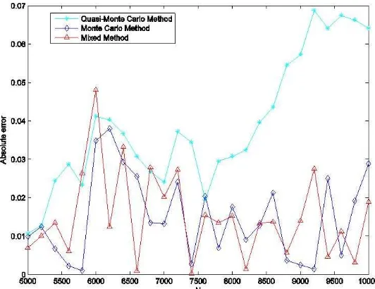
In our tests we considered the dimensions= 32 of the transformed integral (17) on [0,1]s. The MC and H-mixed estimates are the mean values of 10 independent runs, while the QMC estimate is the result of a single run. The results are presented in Figure 1,where the number of samples N varies from 5000 to 10000 with a step of 200.
Figure 1: Simulation results for s= 32 and d= 10 for the Up-and-Out barrier call option.
We can conclude that our mixed method can give considerable improvements over the MC method in almost half of the situations and over the QMC method in almost all of the situations, in estimating Up-and-Out barrier options driven by L´evy processes. Also, the absolute errors for all three estimates are very small, even for small sample sizes.
4.3 Double Knock-Out barrier options
We assume that the initial stock price isS(0) = 110, the strike price isK= 100, the upper barrier price is L = 120 , the lower barrier price is l = 90 and the risk-free annual interest rate isr = 3.75%. We choose the parameter of the double-exponential distributionλ= 95.2271.
We are going to compare the three estimates in terms of their absolute error, where the ”exact” barrier option price is obtained as the average of 10 MC simula-tions, with N = 400000 for the initial integral.
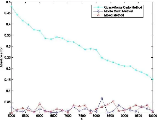
Figure 2: Simulation results fors= 32 andd= 10 for the Double Knock-Out barrier call option.
with a step of 200.
We performed numerical tests for different values of d. We noticed that, to achieve a good performance of the mixed method, the value of d should be 10, which is around one third of the dimension of the problem and which confirms the conclusions from paper [19] concerning the choice of d.
References
[1] O. E. Barndorff-Nielsen, Processes of normal invers Gaussian type, Finance and Stochastic, 2 (1998), 41-68.
[2] P. P. Boyle, Options:A Monte Carlo Approach, J. Financial Economics, 4 (1977), 323-338.
[3] P. Chelson, Quasi-Random Teqniques for Monte Carlo Methods, Ph.D. Dis-sertation, The Claremont Graduate School, 1976.
[4] I. Deak,Random Number Generators and Simulation, Akademiai Kiado, Bu-dapest, 1990.
[5] F. Delbaen, W. Schachermayer,A general version of the fundamental theorem of assest pricing, Math. Ann., 300(3) (1994), 463-520.
[6] L. Devroye,Non-Uniform Random Variate Generation, Springer-Verlag, New-York, 1986.
[7] E. Eberlein, U. Keller,Hyperbolic distribution in finance, Bernoulli, 1 (1995), 281-299.
[8] P. Glasserman, Monte Carlo Methods in Financial Engineering, Springer-Verlag, New-York, 2003.
[9] M. Gnewuch, A. V. Ro¸sca, On G-discrepancy and mixed Monte Carlo and quasi-Monte Carlo sequences, Acta Universitatis Apulensis, Mathematics-Informatics, No. 18 (2009), 97-110.
[10] J. H. Halton, On the efficiency of certain quasi-random sequences of points in evaluating multidimensional integrals, Numer. Math., 2 (1960), 84-90.
[11] E. Hlawka,Gleichverteilung und Simulation, ¨Osterreich. Akad. Wiss. Math.-Natur. Kl. Sitzungsber. II, 206 (1997), 183-216.
[12] E. Hlawka, R. M¨uck, A transformation of equidistributed sequences, Appli-cations of number theory to numerical analysis, Academic Press, New-York, 1972, 371-388.
[13] C. Joy, P. P. Boyle, K. S. Tan, Quasi-Monte Carlo Methods in Numerical Finance, Management Science, Vol. 42, No. 6 (1996), 926-938.
[14] R. F. Kainhofer,Quasi-Monte Carlo algorithms with applications in numeri-cal analysis and finance, Ph.D. Dissertation, Graz University of Technology, Austria, 2003.
[15] I. Nelken,The Handbook of Exotic Options: Instruments, Analysis and Ap-plications, McGraw-Hill, New-York, 1996.
[16] S. Ninomya, S. Tezuka,Toward real time pricing of complex finacial deriva-tives, Applied Mathematical Finance, Vol. 3 (1996), 1-20.
1999.
[18] S. Raible, L´evy Processes in Finance: Theory, Numerics and Empirical Facts, Ph.D. Dissertation, Albert-Ludwigs-Universitat, Freiburg, 2000.
[19] A. V. Ro¸sca, A Mixed Monte Carlo and Quasi-Monte Carlo Sequence for Multidimensional Integral Estimation, Acta Universitatis Apulensis, Mathematics-Informatics, No. 14 (2007), 141-160.
[20] N. Ro¸sca, A Combined Monte Carlo and Quasi-Monte Carlo Method for Estimating Multidimensional Integrals, Studia Universitatis Babes-Bolyai, Mathe-matica, Vol. LII, No. 1 (2007), 125-140.
[21] N. C. Ro¸sca, A Combined Monte Carlo and Quasi-Monte Carlo Method with Applications to Option Pricing, Acta Universitatis Apulensis, Mathematics-Informatics, No. 19 (2009), 217-235.
[22] T. H. Rydberg, The normal inverse Gaussian L´evy process: simulation and approximation, Comm. Statist. Stochastic Models, Vol.13, No. 4 (1997), 887-910.
[23] D. D. Stancu, Gh. Coman, P. Blaga,Numerical Analysis and Approximation Theory, Vol. II, Presa Universitara Clujeana, Cluj-Napoca, 2002 (In Romanian). Alin V. Ro¸sca
Faculty of Economics and Business Administration Babe¸s-Bolyai University
Str. Teodor Mihali, Nr. 58-60, Cluj-Napoca, Romania email:[email protected]
Natalia C. Ro¸sca
Faculty of Mathematics and Computer Science Babe¸s-Bolyai University