Electronic Journal of Qualitative Theory of Differential Equations Proc. 8th Coll. QTDE, 2008, No. 61-10;
http://www.math.u-szeged.hu/ejqtde/
NEIMARK-SACKER BIFURCATION IN A DISCRETE
DYNAMICAL MODEL OF POPULATION GENETICS
ATTILA D´ENES
Abstract. In this paper we investigate a genetic model initiated by G´abor Tusn´ady. This model is a four-dimensional system of difference equations which describes the change of distribution of genotypes from generation to generation in the case of one locus and four alleles considering selection and mutation. During computer experiments Tusn´ady discovered cyclic behaviour in the evolution of genotypes. Using bifurcation theory we prove that the system indeed can have cycles and this occurrence is caused by a Neimark-Sacker bifurcation.
1. Introduction
G. Tusn´ady established a discrete population dynamical model which describes the change of distribution of genotypes from generation to generation considering selection, mutation and recombination.
The genetical program is stored in the cells of living beings in the form of chromo-somes. One half of the chromosomes comes from the mother, the other half comes from the father, i. e., chromosomes appear in pairs. When such adiploidcell divides, each chromosome doubles and the two arising cells get the whole chromosome set. Our organism also containshaploid cells, in which only half as much chromosomes can be found: these are thegametes. These cells originate from diploid cells during meiosiswhich splits chromosome pairs. During fertilization gametes unite and the original chromosome number is re-established. The segments of the chromosomes that determine the different properties are calledgenes, their different variants are called alleles and their place in the chromosomes are called loci. The genotype is determined by the two alleles which are really present in the cell. The distribu-tion of the genoytpes is affected mainly byselection,mutation andrecombination. Selection means that different genotypes have different chances to create offspring. The succesfulness of a genotype is shown by thefitness. When a diploid cell divides and chromosomes double, their copying is not always absolutely precise: certain segments of the chromosome can change, an allele can change to another one. This phenomenon is called mutation. (For details see e. g. [1].)
In Section 2 we introduce Tusn´ady’s model in the case of one locus and four alle-les. Using monograph [2], in Section 3 we delineate the Neimark-Sacker bifurcation and its conditions (Theorem A). In the proof of our main result (Theorem 4.1) we have to use a special procedure to check the genericity conditions of Theorem A. To make our paper self-contained we include this procedure from [2]. In Section 4 we apply the procedure presented in Section 3 to obtain our main result.
2. The model
Let us model the above-mentioned notions mathematically in the case of one locus. Let n denote the number of alleles. Letxi denote the density of the i-th allele in the given generation,x1+...+xn= 1. Let Γ denote the set of genotypes. Then aγ∈Γ genotype is a vector with two independent allele components. Fitness is a mapping from Γ to the [0,1] closed interval. Meiosis is a random mapping from Γ into the set of alleles.
Tusn´ady assumed that mutation depends on both parental genes and created the following model:
Letw(i, j) denote the fitness of the genotypeij, i. e., the probability of genotype
ijcreating offspring and{yij}ni,j=1denotes the distribution of genotypes in the next generation. If we consider selection only, we get the following selection model:
(2.1) yij =
w(i, j)xixj Pn
p,q=1w(p, q)xpxq
.
Let us now consider mutation as well. LetMij(k) denote the probability of the event that a gamete of type k issues from a cell of genotype ij. Mij(k) contains mutation as well. Then, after meiosis, the new distribution of gametes is given by the following formula:
x′k= n X i,j=1
yijMij(k).
If we substitute the expression from the selection model (2.1) in the place ofyij introducing the notationa(i, j, k) =w(i, j)Mij(k), we get the following model:
(2.2) x′k=
Pn
i,j=1a(i, j, k)xixj Pn
i,j,k=1a(i, j, k)xixj
.
Tusn´ady investigated what can be said about the limit sets of the solutions of (2.2) obtained by iterating the mapping and whether there is a system in which there are solutions having more than one limit points. After a long numeric searching he found the following four-dimensional system:
a(2,4,1)=1042 a(2,4,2)=8 a(3,4,2)=113 a(1,2,3)=19 a(2,3,3)=9 a(1,3,4)=1078, a(2,2,4)=414
wherea(i, j, k) =a(j, i, k) and the coefficients not mentioned here are equal to zero. That is, our system is as follows:
(2.3) F(x) =
2084x2x4
38x1x2+414x22+2156x1x3+18x2x3+2100x2x4+226x3x4,
16x2x4+226x3x4
38x1x2+414x22+2156x1x3+18x2x3+2100x2x4+226x3x4,
38x1x2+18x2x3
38x1x2+414x22+2156x1x3+18x2x3+2100x2x4+226x3x4,
414x2
2+2156x1x3
38x1x2+414x22+2156x1x3+18x2x3+2100x2x4+226x3x4
.
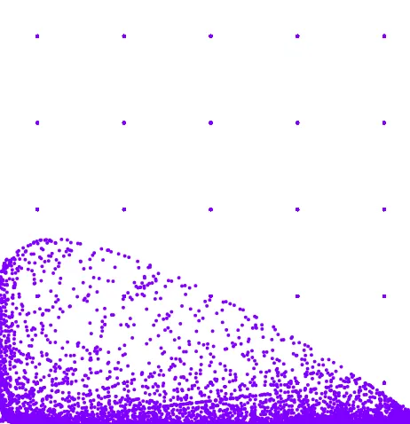
Figure 1. p= 8
Using bifurcation theory we prove that the appearance of the one-dimensional limit is not caused by errors of numeric calculating.
Let us examine the attractor of our system at different parameter values. We chose the coefficient p = a(2,4,2) = a(4,2,2) as a parameter. In Figure 1 the attractor of the system can be seen with the coefficients determined by Tusn´ady.
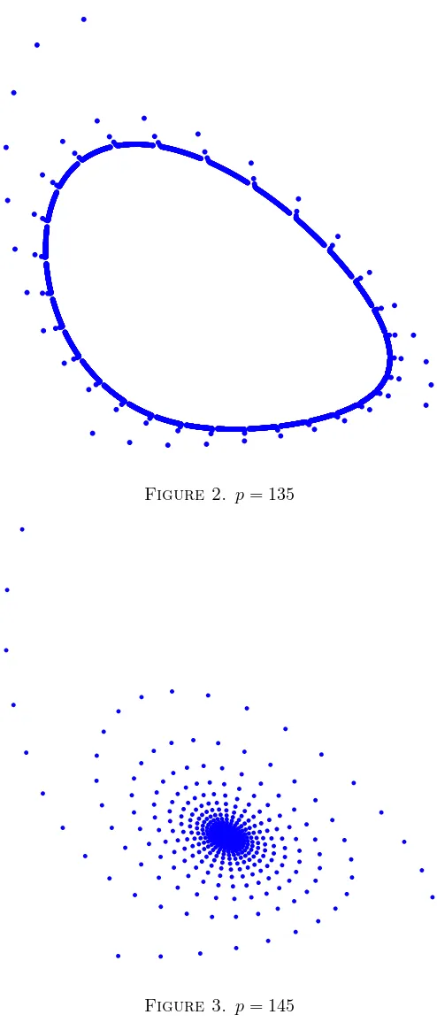
Figure 2 represents the attractor at p = 135, where the attractor is a stable closed curve, while in Figure 3, at p = 145 the attractor is a stable fixed point. The figures suggest that between the last two parameter values a Neimark-Sacker bifurcation takes place, as we can see a stable closed curve arising from the stable fixed point.
Figure 2. p= 135
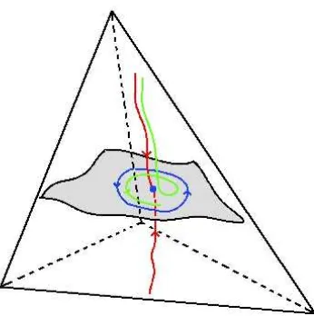
Figure 4. Dynamics of the system
3. Neimark-Sacker bifurcation (see [2, Sections 4.7, 5.4])
If we change parameterp=a(2,4,2) =a(4,2,2), a complex pair of eigenvalues of the Jacobian of the system passes through the unit circle. However, the system has to satisfy some non-degenericity conditions to ensure a Neimark-Sacker bifurcation. First we formulate the Neimark-Sacker bifurcation theorem for two-dimensional systems.
Let us consider the following two-dimensional system:
x7→f(x, α), x∈R2, α∈R1,
where the smooth function f has at α = 0 the fixed point x = 0 with simple eigenvaluesµ1,2=e±iθ0,0< θ0< π. By the Implicit Function Theorem, the system has a unique fixed pointx0(α) for all sufficiently small|α| in some neighbourhood of the origin, since µ = 1 is not an eigenvalue of the Jacobian matrix. With a parameter-dependent coordinate shift we can place the fixed point at the origin, therefore we can assume that x = 0 is the fixed point for |α| sufficiently small. Thus, the system can be written as
(3.1) x7→A(α)x+F(x, α),
whereFis a smooth vector function and its componentsF1,2have Taylor expansions inxstarting with at least quadratic terms,F(0, α) = 0 for all sufficiently small|α|. The Jacobian matrixA(α) has two multipliers
µ1,2=r(α)e±iϕ(α),
and express the multipliers in terms of β: µ1(β) = µ(β), µ2(β) = µ(β), where
µ(β) = (1 +β)eθ(β)andθ(β) is a smooth function such thatθ(0) =θ0.
To formulate the theorem we need another transformation. Omitting the tech-nical details it is enough to say that introducing a complex variable and a new parameter system (3.1) can be transformed for all sufficiently small |α| into the following form:
z7→µ(β)z+g(z, z, β),
where β ∈ R1, z ∈ C1, µ(β) = (1 +β)eiθ(β) and g is a smooth complex-valued function of z, z and β, whose Taylor expansion with respect to (z, z) contains quadratic and higher-order terms:
g(z, z, β) = X k+l≥2
1
k!l!gkl(β)z kzl,
k, l= 0,1, . . . .
Now we can state the following theorem for Neimark-Sacker bifurcation in two dimensions:
Theorem A (Generic Neimark-Sacker bifurcation ([2])). For any generic two-dimensional one-parameter system
x7→f(x, α),
having at α= 0 the fixed point x0 = 0with complex multipliers µ1,2=e±iθ0 there is a neighbourhood of x0 in which a unique closed invariant curve bifurcates from
x0 asαpasses through zero.
The system has to satisfy the following genericity conditions: (1) r′(0)6= 0, whereµ1,2(α) =r(α)e±iϕ(α),r(0) = 1, ϕ(0) =θ0, (2) e±ikθ06= 1,
k= 1,2,3,4,
(3) a(0)6= 0, wherea(0) = Ree−iθ0g21
2
−Re(1−2e
iθ0)e−2iθ0
2(1−eiθ0) g20g11
−12|g11|2− 1
4|g02|
2, where g
ij =gij(0).
Coefficient a(0) in condition (3) determines the direction of the appearance of the invariant curve in a generic system exhibiting Neimark-Sacker bifurcation. If
a(0) is negative, the bifurcation is supercritical, i. e., a stable closed invariant curve bifurcates from a stable fixed point while the fixed point becomes unstable. Ifa(0) is positive, the bifurcation is subcritical, i. e., an unstable closed curve disappears as we pass through the critical value.
As for systems with dimension higher than 2 essentially the same takes place: there exists a two-dimensional invariant manifold on which the system exhibits the bifurcation, while the behaviour off the manifold is “trivial”.
During the proof of Theorem 2.1 we followed the procedure described in [2]. Using this method we avoid the transformation of the system into its eigenbasis. We use the eigenvectors belonging to the critical eigenvalues of the Jacobian A
We write the system in the form
(3.2) G(x) =Ax+H(x), x∈R,
whereH(x) =O(kxk2) is a smooth function with Taylor expansion
H(x) = 1
2B(x, x) + 1
6C(x, x, x) +O(kxk 4)
,
whereB(x, x) andC(x, x, x) are multilinear functions. In coordinates:
(3.3) Bi(x, y) = n X j,k=1
∂2Hi(ξ)
∂ξj∂ξk ξ=0
xjyk
and
(3.4) Ci(x, y, z) = n X j,k,l=1
∂3Hi(ξ)
∂ξj∂ξk∂ξl ξ=0
xjykzl,
wherei= 1,2, . . . , n.
Ahas a simple pair of complex eigenvalues on the unit circle: µ1,2=e±iθ0 Letq∈Cn denote the complex eigenvector corresponding to µ1:
(3.5) Aq=eiθ0
q, Aq=e−iθ0 q.
Introduce also the adjoint eigenvectorp∈Cn which has the property (3.6) ATp=e−iθ0
p, ATp=eiθ0 q.
and satisfies the normalizationhp, qi= 1.
The critical real eigenspaceTc corresponding to µ
1,2 is two-dimensional and is spanned by Req,Imq. The real eigenspace Tsu corresponding to all other eigen-values ofA is (n−2)-dimensional. y ∈Tsu if and only ifhp, yi= 0. As y∈Rn is real andp∈Cn is complex, the conditionhp, yi= 0 implies two real constraints on
y. We decomposex∈Rn as
x=zq+zq+y,
wherez∈C1 andzq+zq∈Tc,y∈Tsu. We have
z =hp, xi
y =x− hp, xiq− hp, xiq.
After a series of transformations we get the following form for the map: (3.7) z˜=eiθ0
z+1 2g20z
2+g
11zz+1 2g02z
2+1 2g21z
2z+· · ·, where
and
g21=hp, C(q, q, q) + 2hp, B(q,(E−A)−1
B(q, q)))i+hp, B(q,(e2iθ0
E−A)−1
B(q, q))i
+ e
−iθ0(1−2eiθ0)
1−eiθ0 hp, B(q, q)ihp, B(q, q)i
− 2
1−e−iθ0|hp, B(q, q)i|
2− eiθ0
e3iθ0−1|hp, B(q, q)i|
2
.
Ifeikθ0 6= 1 for
k= 1,2,3,4,we can transform (3.7) into the following form: ˜
z=eiθ0z(1 +
d(0)|z|2) +O(|z|4).
Here the real numbera(0) = Red(0) determines the direction of bifurcation of a closed invariant curve, and can be obtained from the following formula:
a(0) = Re
e−iθ0 g21 2
−Re
(1−2eiθ0) e−2iθ0
2(1−eiθ0) g20g11
− 1
2|g11| 2−1
4|g02| 2
.
Using this formula with the above-definded coefficients, we obtain the following invariant expression:
a(0) = 1 2Re
e−iθ0
hp, C(q, q, q)i+ 2hp, B(q,(E−A)−1B(q, q))i
+hp, B(q,(e2iθ0
E−A)−1B(q, q))i .
(3.9)
This formula allows us to verify the nondegeneracy of the nonlinear terms at a nonresonant Neimark-Sacker bifurcation ofn-dimensional maps withn≥2.
4. Main result
Theorem 4.1. Tusn´ady’s system (2.3) undergoes a Neimark-Sacker bifurcation at parameter value 139.455, i. e., a stable invariant closed curve bifurcates from a stable fixed point while the fixed point becomes unstable.
Proof:
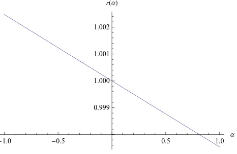
To check condition (1) of Theorem A we calculated the value ofr′(0) numerically
and obtainedr′(0) =−0.00217713. (Actually, to check the transversality directly,
we draw the graph of the interpolating function tor, see Figure 5.)
The critical eigenvalues are 0.561391 + 0.827552iand 0.561391−0.827552i, i. e., they are not complex roots of unity of order four or less and condition (2) of Theorem A is satisfied.
-1.0 -0.5 0.5 1.0
Α
0.999 1.000 1.001 1.002
[image:9.595.192.425.120.272.2]rHΑL
Figure 5. Interpolating function tor
We determine the eigenvectorqand the adjoint eigenvectorpintroduced in (3.5) and (3.6):
q= (−0.67126−0.0108908i,−0.0793651−0.049971i,
0.0181909 + 0.0608618i,0.732434 +i)
p= ( 0.0134851−0.0321706i,−0.19597−0.00610824i,
0.97727,−0.0340428 + 0.0642307i)
Now we have to compute the functionsB andC introduced in (3.3) and (3.4). Here we only showB1 andC1; the rest of the functions look similar to these.
B1(x, y) =
0.281071x1y1+ 1.3569x2y1−4.99837x3y1+ 0.337012x4y1+ 1.3569x1y2−30.0461x2y2+ 42.9415x3y2−1.51484x4y2− 4.99837x1y3+ 42.9415x2y3+ 208.644x3y3+ 7.85539x4y3+ 0.337012x1y4−1.51484x2y4+ 7.85539x3y4−2.8086x4y4
C1(x, y, z) =
0.413396x1y1z1+ 3.40342x2y1z1−13.5565x3y1z1+ 0.961551x4y1z1+ 3.40342x1y2z1+ 6.19157x2y2z1+ 28.8248x3y2z1−1.50999x4y2z1− 13.5565x1y3z1+ 28.8248x2y3z1−369.354x3y3z1+ 10.0174x4y3z1+ 0.961551x1y4z1−1.50999x2y4z1+ 10.0174x3y4z1+ 0.136465x4y4z1+ 3.40342x1y1z2+ 6.19157x2y1z2+ 28.8248x3y1z2−1.50999x4y1z2+ 6.19157x1y2z2−696.409x2y2z2+ 234.526x3y2z2−13.6853x4y2z2+ 28.8248x1y3z2+ 234.526x2y3z2+ 2845.51x3y3z2−41.4316x4y3z2− 1.50999x1y4z2−13.6853x2y4z2−41.4316x3y4z2−0.0275582x4y4z2− 13.5565x1y1z3+ 28.8248x2y1z3−369.354x3y1z3+ 10.0174x4y1z3+ 28.8248x1y2z3+ 234.526x2y2z3+ 2845.51x3y2z3−41.4316x4y2z3− 369.354x1y3z3+ 2845.51x2y3z3+ 8360.91x3y3z3+ 642.894x4y3z3+ 10.0174x1y4z3−41.4316x2y4z3+ 642.894x3y4z3+ 0.598556x4y4z3+ 0.961551x1y1z4−1.50999x2y1z4+ 10.0174x3y1z4+ 0.136465x4y1z4− 1.50999x1y2z4−13.6853x2y2z4−41.4316x3y2z4−0.0275582x4y2z4+ 10.0174x1y3z4−41.4316x2y3z4+ 642.894x3y3z4+ 0.598556x4y3z4+ 0.136465x1y4z4−0.0275582x2y4z4+ 0.598556x3y4z4−18.9188x4y4z4
With the help of these functions we can calculate the values of the scalar products in the formula fora(0).
For the value ofa(0) at parameter value 139.455 we get−13.9966. Asa(0)6= 0, the system is non-degeneric, i. e., there is a Neimark-Sacker bifurcation taking place at parameter value 139.455. As a(0) is negative, the bifurcation is supercritical, i. e., a stable closed invariant curve bifurcates from the fixed point while the fixed point becomes unstable.
5. Acknowledgement
The author is grateful for the suggestions and comments by the referee that helped to improve the paper.
References
[1] Hofbauer, S., Sigmund, K.,Evolutionary Games and Population Dynamics, Cambridge University Press, 1998.
[2] Kuznetsov, Y. A.,Elements of applied bifurcation theory, Springer-Verlag, 1998. [3] Tusn´ady, G., Mut´aci´o ´es szelekci´o,Magyar Tudom´any 7(1997), 792–805. [4] Wiggins, S.,Global Bifurcations and Chaos, Springer-Verlag, New York, 1988.
(Received September 13, 2007)