Full Terms & Conditions of access and use can be found at
http://www.tandfonline.com/action/journalInformation?journalCode=ubes20
Download by: [Universitas Maritim Raja Ali Haji] Date: 11 January 2016, At: 22:50
Journal of Business & Economic Statistics
ISSN: 0735-0015 (Print) 1537-2707 (Online) Journal homepage: http://www.tandfonline.com/loi/ubes20
Improving Real-Time Estimates of Output and
Inflation Gaps With Multiple-Vintage Models
Michael P. Clements & Ana Beatriz Galvão
To cite this article: Michael P. Clements & Ana Beatriz Galvão (2012) Improving Real-Time
Estimates of Output and Inflation Gaps With Multiple-Vintage Models, Journal of Business & Economic Statistics, 30:4, 554-562, DOI: 10.1080/07350015.2012.707588
To link to this article: http://dx.doi.org/10.1080/07350015.2012.707588
View supplementary material
Accepted author version posted online: 05 Jul 2012.
Submit your article to this journal
Article views: 205
Supplementary materials for this article are available online. Please go tohttp://tandfonline.com/r/JBES
Improving Real-Time Estimates of Output
and Inflation Gaps With Multiple-Vintage Models
Michael P. C
LEMENTSDepartment of Economics, University of Warwick, Coventry, United Kingdom ([email protected])
Ana Beatriz G
ALVAO˜
Department of Economics, Queen Mary University of London, London, United Kingdom ([email protected])
Real-time estimates of output gaps and inflation gaps differ from the values that are obtained using data available long after the event. Part of the problem is that the data on which the real-time estimates are based is subsequently revised. We show that vector-autoregressive models of data vintages provide forecasts of post-revision values of future observations and of already-released observations capable of improving estimates of output and inflation gaps in real time. Our findings indicate that annual revisions to output and inflation data are in part predictable based on their past vintages. This article has online supplementary materials.
KEY WORDS: Data revisions; Inflation trend; Output gap; Real-time forecasting.
1. INTRODUCTION
Policy makers often require reliable estimates of the current state of the economy. Because national accounts data are subject to revision, current estimates of key macroeconomic variables (such as output growth and inflation) for present and recent peri-ods are provisional: post-revision estimates will not be available until some later date. This raises the question of whether more accurate estimates of these macro-variables can be obtained be-yond simply assuming that the latest-available estimate is the best indicator of the “true” value (taken to be the post-revision value).
Monetary policy perhaps best exemplifies the need to estimate the current state of the economy. Estimates of the current output gap are key, and it has been shown that estimates based on final data can be markedly different from those available in real time, affecting both historical evaluations of monetary policy and the effective conduct of monetary policy in real time (see, e.g., Orphanides2001; Orphanides and van Norden2002). We con-sider the improvements in the accuracy of real-time output gap estimation achievable from first estimating the post-revision val-ues of the relevant data. Models are employed to calculate post-revision estimates of the level of output for current, past, and future observations. We quantify the resulting improvements in output gap estimation. As we detail in the following, a number of ways of forecasting revised data have been proposed. We present an empirical investigation of the relative merits of these approaches along side our preferred model.
Recently, a number of authors have estimated the trend infla-tion rate, associated with either long-run inflainfla-tion expectainfla-tions or a time-varying inflation target. These include contributions by Kozicki and Tinsley (2005), Stock and Watson (2007,2010), and Cogley, Primiceri, and Sargent (2010). Changes in the per-sistence of the inflation gap, defined as the difference between the observed inflation rate and trend inflation, are also important for the conduct of monetary policy (see Cogley, Primiceri, and Sargent2010). Notwithstanding the attention to real-time issues surrounding the estimation of output gaps, we are unaware of
any studies of the real-time estimation of inflation gaps and trends. The literature to date has used fully revised data: our interest is in the quality of estimates that can be obtained in real time, and as for the output gap, whether we can obtain more ac-curate estimates by predicting the future revisions to the relevant data.
The models we use to forecast revisions and post-revision future observations of output growth and inflation are related to the vector-autoregressive (VAR) models by Garratt et al. (2008, 2009) and Hecq and Jacobs (2009). In our models, the elements of the vector of variables being modeled consist of the
vintage-t+1 estimates of the observations for the periodtback tot−
q+1, where the observations are the growth rates (so either the output growth rate, or inflation). The model supposes that these vintage-t+1 growth rate estimates are predictable from earlier vintage estimates (e.g., the vintage-t estimate of observations
t−1 tot−q). We model a three-and-a-half-year release cycle, including initial revisions and three waves of annual revisions, soqis set to 14 for vintages sampled quarterly. This differs from that by Garratt et al. (2008; henceforth GLMS) who specified a cointegrated VAR for the levels of log-output, assuming that only initial revisions are predictable. Our approach is in the spirit of the general unrestricted VAR model by Sims (1980), but we also consider a wide range of related VAR models, including models that reflect more closely the timing of the release of data revisions by the government statistical agency, as well as a model that imposes the restriction that annual and benchmark revisions are unpredictable. We also consider the forecast performance of models based on the approach by Kishor and Koenig (2011; henceforth KK), as an alternative way of allowing for data revisions, and extensions that allow for the seasonal nature of data revisions.
© 2012American Statistical Association Journal of Business & Economic Statistics October 2012, Vol. 30, No. 4 DOI:10.1080/07350015.2012.707588
554
Clements and Galv ˜ao: Improving Real-Time Estimates of Output and Inflation Gaps 555
The unrestricted vintage-based VAR model (henceforth V-VAR) is generally the dominant forecasting model. It provides more accurate forecasts of the fully revised values of past ob-servations (backcasts) in comparison with specifications (such as GLMS) that assume that annual and benchmark revisions are unpredictable. We investigate the extent to which the forecasts from the multiple-vintage models (such as the V-VAR model) improve the accuracy of real-time estimates of output and infla-tion gaps.
The issues we address are part of a wider literature on real-time data analysis, reviewed by Croushore (2011a, 2011b), which includes the analysis of the nature of data revisions (see, e.g., Mankiw and Shapiro 1986; Faust, Rogers, and Wright 2005; Aruoba 2008; Corradi, Fernandez, and Swanson 2009) and forecast evaluation in real time (see, e.g., Faust, Rogers, and Wright2003; Clements and Galv˜ao2008). Our focus is on forecasting the final or fully revised data in such an environment. The plan of the article is as follows. The vintage-based VAR model is described in Section2, along with the other models for forecasting data revisions. Section3 provides evidence on the extent to which data revisions are predictable using V-VAR, the GLMS model, and the KK model. Sections4and5document the extent to which more “accurate data” (i.e., using forecasts of revisions to past data and of revisions to future data, as appropri-ate) translate into improved measures of the output gap and the inflation trend and gap. Section4defines the output gap using the filter by Hodrick and Prescott (1997) (HP) to calculate trend output, but results for an alternative definition are given in the Supplementary Appendix (see supplementary materials posted on the journal web site). Section 5 estimates trend inflation and the inflation gap using the Stock and Watson (2007,2010) model of cycle and trend. Section 6 offers some concluding remarks. The Supplementary Appendix provides details of ad-ditional models, including seasonal variants of the main models, which impose restrictions based on the timing of data releases. These are not found to improve on the models in the main text.
2. MODELS FOR BACKCASTING AND FORECASTING USING PAST DATA VINTAGES
VARs model relationships between observable variables. Other approaches introduce unobserved components (e.g., Jacobs and van Norden2011), which relate a vector of different vintage estimates of yt to the (generally unobserved) true
value and latent news and noise measurement errors (see also Cunningham et al. 2009). As an example of the unobserved components approach, we consider the approach by Kishor and Koenig (2011).
t−1) be the quarterly percentage
change (at an annual rate) for periodt(denoted by the subscript) computed using data vintaget+1 (i.e., the data available at time
t+1, denoted by the superscript), whereYis the natural log of the level of the variable we are interested in (either real GDP, or the price level). Hence,ytt+1 is the first estimate of the growth rate for periodt. If we suppose that there are revisions for the nextq−1 quarters, but thereafter the observation is unrevised
(i.e.,ytt+q+i =y
the dynamics of successive vintages of data that include both a new observationyt+1
t and revised estimates of past
observa-tionsytt−+11, . . . , ytt−+q1+1. The first equation of the VAR refers to first releases,yt+1
t , the second equation to data that has been
re-vised once,ytt−+11, and so on. The variance–covariance matrix of the disturbances (ε=E(εt+1εt+1′)) captures the correlations between data published in the same vintage.
The autoregressive orderpis set to capture serial correlation in yt+1, and in practice it may be possible to set p to a low
value. For example, even settingp=1 allowsyt+1
t to depend
on q lags (all from the period t-data vintage), where in the base case q =14. Ideally, the vector yt+1
should include all revisions. Taking this literally would be impractical as a data point is always subject to further revision, chiefly in the form of benchmark revisions. Setting q=14 is a compromise that explicitly allows for the three annual revisions to which each data point is subject (see, e.g., Fixler and Grimm2005,2008; Landefeld, Seskin, and Fraumeni2008, on Bureau of Economic Analysis (BEA) data releases and revisions).
We consider a restricted V-VAR model based on the belief that after a small number of revisions, further revisions are unpredictable. This greatly reduces the number of parameters that need to be estimated relative to the V-VAR. Suppose that after n−1 revisions, the next estimate yt+n+1
t is an efficient
forecast in the sense that the revision from yt+n
t toyt+n+
In the empirical work, we setn=2 so that values after the first revision (considering vintages are quarterly observed) are as-sumed to be efficient forecasts (i.e., the BEA estimate published two quarters after the period to which it refers is an efficient forecast). An unrestricted intercept is included in each equa-tion, to accommodate nonzero mean revisions. We refer to this model as the “news-restricted” vintage-based VAR, RV-VAR.
To understand the nature of the VAR forecasts, consider the forecast origin t+1. At this time, all the data vintages up to and including the time t+1 vintage are known, that
is,yt+1
forecasts of the first estimate of yt+h, a forecast of the
sec-ond estimate ofyt+h−1, and so on down to theqth estimate of
yt+h−q+1. The forecasts are computed by iteration in the
stan-dard way. The calculation of output and inflation gaps requires “post-revision” values, which we take to be the qth estimate (where usuallyq=14). (Clements and Galv˜ao (2012a) allow that all elements of the vector yt+1+h|t+1 may be of interest.)
This means we only consider forecasts of a subset of the ele-ments ofyt+1+h|t+1, namely, the last elements of each vector for
Following Patterson (2003), GLMS work in terms of the level (of the log) of output (Y), which is taken to be integrated of order one (I(1)), and they assume that different vintage estimates are cointegrated such that data revisions areI(0). Their model is
Zt+1=c+1Zt+2Zt−1+εt, (3)
where
Zt+1−i=Ytt−+i1−i−Ytt−−1i−i, Ytt−+11−−ii−Ytt−−1i−i, Ytt−+21−−ii−Ytt−−2i−i′
fori=0,1,2, and where thei are 3×3 matrices of
coeffi-cients with third columns consisting solely of zeros (see Garratt et al.2008, for details). The first element of Zt+1
is a differ-ence across vintage and observation, and subsequent terms are revisions to past data. The inclusion of two revisions reflects the view that a “revision horizon” of two is appropriate: revi-sions such asYtt−+21−j −Ytt−2−j forj >0 are regarded as being unpredictable.
As already described, our VAR models are formulated in terms of growth rates, and revisions in growth rates. Deciding which is the more appropriate approach from a forecasting per-spective is an empirical issue (see, e.g., Elliott2006; Clements and Hendry2006). However, in the current context an advantage of our approach is that the level shifts due to base-year changes (or to other definitional changes) at times of benchmark revi-sions have no effect on our “same-vintage” growth rates. These shifts cannot be easily handled by the GLMS model, and the level-shift components of the benchmark revisions are removed from the real-time dataset prior to estimating Equation (3). The adjustments we make to the real-time dataset to estimate the GLMS model are as follows (these were suggested in a private communication from Professor K. Lee). LettBLdenote the
vin-tage date of the most recent benchmark revision. The adjustment process assumes that in the absence of the definitional change,
YttBL
data from all the vintages prior totBL are adjusted by a fixed
factor, back to and including the data in the previous benchmark revision vintage,tBL−1. Data in vintages before tBL−1 are then
adjusted by the multiplicative factor (YtBL−1 tBL−1−4/Y
tBL−1−1
tBL−1−4), and so
on. We smooth eight benchmark revisions in this way. Note that both adjusted and unadjusted data provide the same vintage-based data in growth rates, so the data adjustment has no effect on the models described previously.
Garratt et al. (2008, p. 797, footnote 14) noted that they extended their model to allow for seasonal effects from annual revisions to output, but did not find significant improvements in fit. Because they applied their model to output growth but not inflation, we follow their lead and only use the GLMS model for output.
Following Garratt et al. (2008), we compute forecasts for log-levels
Ytt++h1+h|t+1, Ytt−+11++hh|t+1, Ytt−+21++hh|t+1′
using OLS estimates of Equation (3). Then growth rate forecasts are computed as
ytt+−11++hh|t+1=400Ytt−+11++hh|t+1−Ytt−+21++hh|t+1
to compare with other multiple-vintage models.
Note that we can only compute backcasts based on the spec-ification in Equation (3) for the first releaseyt+1
t , that is, given
data vintaget+1 we can forecastytt+3|t+1, but not earlier
ob-servations (such asyt−1, etc.).
2.3 The Kishor and Koenig Approach
Kishor and Koenig (2011) modeled the “final data” by an au-toregressive model, with equations for the measurement errors. Their modeling approach encompasses the approaches by both Howrey (1978) and Sargent (1989) in terms of the assumptions made about the nature of data revisions. They assumed that af-ter a finite number of revisions the estimates are fully efficient. Their approach is appealing in that it does not make restrictive assumptions about the nature of data revisions, and the model can be extended to allow for the seasonal nature of data revi-sions. Their empirical forecasting exercises are based on annual observations, which require only a small number of revisions before releases are efficient, and they considered one-step-ahead forecasts of future observations. They found improved forecasts of output growth in comparison with the traditional real-time approach, but not for inflation.
Our interest is in forecasting revisions to past data as well fu-ture data at multiple steps ahead. The labeling of this model as “KK” should not be taken to imply it is how Kishor and Koenig (2011) would necessarily proceed. Define yt =
[yt, . . . , yt−q+1]′as a vector of true values of the same
dimen-sion asyt+1. The last element ofyt+1can be assumed to either
equal the final value (i.e.,ytt−+q1+1=yt−q+1) or to be an efficient
estimate of it. The model can be written succinctly in state-space
Clements and Galv ˜ao: Improving Real-Time Estimates of Output and Inflation Gaps 557
form with measurement and state equations:
yt+1=[Iq Iq]
where Iq is the identity matrix of order q. The disturbances
vectors arevt =(v1t,0, . . .0)′andεt =(ε1t, . . . , εq−1t,0)′. As
shown by KK, in the general case the errors in the data revision equationsεtwill be correlated with the disturbances to the true
values,v1t, as well as being contemporaneously correlated. We
definevt =(vt,εt)′ , and let E(vtv′t)=Q. Theq×1 vectors
c1 andc2arec1=(c1,0, . . . ,0)′andc2=(c21, . . . , c2q−1,0)′.
The true valuesyt follow an autoregression of orderp, defined
by the first block of Equation (5) with
F=
The matrixKdescribes the dynamics ofq−1 data revisions
yt+1−y
seemingly unrelated regression estimator. Becauseyt consists
of final values, given the assumption thatytt−+1q++i1=yt−q+1 for
i≥0, the estimation sample ends att =T −q+1 whenT +1 is the forecast-origin data vintage. Application of the Kalman Filter then provides backcasts (i.e., of the post-revision values of current and past observations,yt−q+2up toyt). Forecasts of
post-revision future observationsyt+1,. . .,yt+Hare obtained by
iterating the state equation conditional onˆyTforh=1, . . . , H.
Our baseline model setsq =14 andp=4, and we allowKto be an unrestricted coefficient matrix (with (q−1)2parameters). We also consider a range of related model, including specifica-tions with diagonalKand seasonal specifications. Details of these models and forecasting results are in the Supplementary Appendix.
2.4 A Single-Equation Approach
The V-VAR is also closely related to the single-equation approach by Koenig, Dolmas, and Piger (2003). The first equation of Equation (1) withp=1 is the “real-time-vintage” autoregression by Clements and Galv˜ao (2012b), labeled
AR-RTV: release valueyTT++12, this approach is preferable in some circum-stances to the traditional approach of simply estimating an AR model on the data in the latest-available vintage (T +1), that is, to estimatingyT+1
t =α0+
pAR
i=1αiytT−+i1+ζtont=2, . . . , T.
Because our interest is in forecasting post-revision values, we follow the suggestion by Clements and Galv˜ao (2012b) to correct the forecast from Equation (6) by the sample estimate of the mean revision ytt+q−ytt+1 for t through T +1−q.
Because the VAR is estimated equation-by-equation by OLS, the estimates of the coefficients in the first equation (first row) of Equation (1) will be the same as the AR estimated with real-time-vintage data whenpAR=q. In the empirical exercise in
Section3, we use Equation (6) as a benchmark against which the V-VAR model forecasts of future observations can be evaluated.
3. FORECASTING FINAL DATA OF OUTPUT GROWTH AND INFLATION
The models we consider are the unrestricted vintage-based VAR (V-VAR), the RV-VAR that assumes that annual and bench-mark revisions are unpredictable except by a nonzero mean (RV-VAR), the GLMS model, and the KK model. Models that explicitly take into account the seasonal nature of data releases do not improve on the V-VAR, and to save space results for such models are confined to the Supplementary Appendix.
Recall that the benchmark model for forecasts of post-revision values of future observations is the single equation model in Equation (6). For forecasting future data releases of past ob-servations, the benchmark is simply that revisions are assumed to be zero. By comparing the accuracy of the forecasts of data revisions from the vintage-based VAR models with the forecasts from the no-change benchmark, we can assess the predictability of data revisions. The RV-VAR model is expected to do bet-ter than the benchmark for moderate and heavily revised data if revisions are nonzero mean. If the V-VAR outperforms the RV-VAR, then the annual and benchmark revisions are in part predictable. In terms of forecasting future observations, we are interested in whether the use of multiple-data vintages leads to superior forecasts, and if the choice of multiple-vintage model (V-VAR, GLMS and KK) matters.
We use real-time data on real output and the GDP deflator published by the Philadelphia Fed (see Croushore and Stark 2001). We have at our disposal 178 data vintages from 1965:Q4 up 2010:Q1 to estimate the models and evaluate their relative forecast performance. The models are initially estimated on the data vintages from 1965:Q4 to 1985:Q3, and then on vintages from 1965:Q4 to 1985:Q4, and so on up to 1965:Q4 to 2006:Q3, adopting an expanding window of data approach (i.e., “recursive forecasting”). We stop at the 2006:Q3 vintage in order that the forecasts can be compared to “actual” values from the 2010:Q1 data vintage that can be regarded as fully revised.
We set h∗=25 (see Section 2.1) that gives forecasts of post-revision values of data up to yt+12 (the last element of
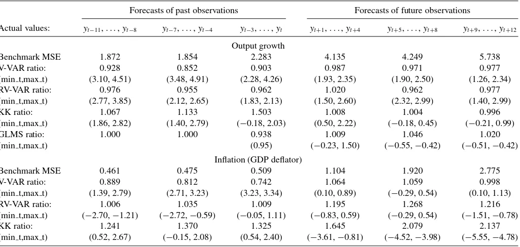
Table 1. The accuracy of forecasts of post-revision output growth and inflation
Forecasts of past observations Forecasts of future observations
Actual values: yt−11,. . .,yt−8 yt−7,. . .,yt−4 yt−3,. . .,yt yt+1,. . .,yt+4 yt+5,. . .,yt+8 yt+9,. . .,yt+12
Output growth
Benchmark MSE 1.872 1.854 2.283 4.135 4.249 5.738 V-VAR ratio: 0.928 0.852 0.903 0.987 0.971 0.977 (min t,max t) (3.10, 4.51) (3.48, 4.91) (2.28, 4.26) (1.93, 2.35) (1.90, 2.50) (1.26, 2.34) RV-VAR ratio: 0.976 0.955 0.962 1.020 0.962 0.977 (min t,max t) (2.77, 3.85) (2.12, 2.65) (1.83, 2.13) (1.50, 2.60) (2.32, 2.99) (1.40, 2.99) KK ratio: 1.067 1.133 1.503 1.008 1.004 0.996 (min t,max t) (1.86, 2.82) (1.40, 2.79) (−0.18, 2.03) (0.50, 2.22) (−0.18, 0.45) (−0.21, 0.99) GLMS ratio: 1.000 1.000 0.938 1.009 1.046 1.020 (min t,max t) (0.95) (−0.23, 1.50) (−0.55,−0.42) (−0.51,−0.42)
Inflation (GDP deflator)
Benchmark MSE 0.461 0.475 0.509 1.104 1.920 2.775 V-VAR ratio: 0.889 0.812 0.742 1.064 1.059 0.998 (min t,max t) (1.39, 2.79) (2.71, 3.23) (3.23, 3.34) (0.10, 0.89) (−0.29, 0.54) (0.10, 1.13) RV-VAR ratio: 1.006 1.035 1.009 1.195 1.268 1.216 (min t,max t) (−2.70,−1.21) (−2.72,−0.59) (−0.05, 1.11) (−0.83, 0.59) (−0.29, 0.54) (−1.51,−0.78) KK ratio: 1.241 1.370 1.325 1.645 2.079 2.137 (min t,max t) (0.52, 2.67) (−0.15, 2.08) (0.54, 2.40) (−3.61,−0.81) (−4.52,−3.98) (−5.55,−4.78)
NOTE: Forecasts are calculated recursively with the vintaget+1=1985:Q3 as the first forecast origin, ending witht+1=2006:Q3. Forecast accuracy is calculated relative to final values of the actuals (taken from the 2010:Q1 vintage). The table reports the MSE of the benchmark forecasts (“no change” for past observations, the AR-RTV for future observations). For V-VAR, RV-VAR, KK, and GLMS, the MSE for the selected set of forecast horizons (equivalently, data maturities) is reported as a ratio of the benchmark MSE for those horizons. Section 2 includes description of how forecasts are computed for each model. The figures in parentheses are the minimum and maximum values of the Clark and West (2007) test of equal predictive accuracy relative to the benchmark, across the four horizons.
the forecast vector when h=25 is ytt++121+25|t+1), and of the post-revision values of the observation at the forecast origin (ytt+1+13|t+1) and of the previous 12 observations back to
ytt+−121+1|t+1. This results in 85 sequences of forecasts of the fully revised values of{yt−12, yt−11, . . . , yt+12}. We split these
fore-casts and their associated forecast errors into three sets for “past data,” {yt−11, . . . , yt−8}, {yt−7, . . . , yt−4}, and {yt−3, . . . , yt},
and into three sets for “future data”, {yt+1, . . . , yt+4},
{yt+5, . . . , yt+8}, and {yt+9, . . . , yt+12}. Forecasts from the
GLMS model are based onh=1, . . . ,13 (see Section 2.2), and from the KK model withh=1, . . . ,12 for future observations and filtered values for backcasting (see Section 2.3).
Table 1reports the benchmark mean squared forecast error (MSFE) for each forecasting horizon set, as well as the ratio of each models’ MSFE to the benchmark. We also calculate the Clark West (2007) test of equal accuracy for each{yt+j},
j = −11, . . . ,+12, and record the minimum and maximumt -statistics overjfor each set. This is an asymptotically normally distributed test of equal predictive accuracy recommended for nested models. Consider backcasts of output growth. The av-erage MSFE of the V-VAR for forecasting lightly revised data, namely {yt−3, . . . , yt}, is 0.903 of the benchmark MSFE,
in-dicating a 10% improvement in forecast accuracy on average across the four target periods. The minimumt-statistic is 2.28, which is significant at the 5% level, so that for all four tar-get periods we reject the null that the V-VAR model forecasts are no more accurate than those of the no-change benchmark. For the more mature data{yt−7, . . . , yt−4}, we find larger gains
in forecast accuracy (relative to the no-change benchmark) of around 15%. For inflation, V-VAR forecasts of lightly revised data ({yt−3, . . . , yt}) are 25% more accurate. It is apparent that
the V-VAR backcasts are statistically significantly more accu-rate than the benchmark for both inflation and output growth. In terms of forecasting future observations, the V-VAR offers small improvements on MSFE for output growth, but not for inflation. The RV-VAR is generally dominated by the V-VAR for both variables: imposing the restriction that revisions after the first are unpredictable has a negative impact in terms of out-of-sample forecasting. Our implementation of KK is at best on par with the benchmark forecasts, and GLMS is dominated by the V-VAR for output growth. Our results indicate greater pre-dictability of U.S. data revisions than has typically been found (see, e.g., Faust, Rogers, and Wright2005), but the literature focuses on revisions from first to final estimates, whereas for our purposes revisions to data of varying degrees of maturity are relevant. For output growth, some of the largest gains (relative to the benchmark) are to the more mature data.
In the Supplementary Appendix, we investigate whether the relative accuracy of the models has been roughly constant over the whole out-of-sample period. There is some evidence that data revisions to output growth are harder to forecast toward the end of the out-of-sample period. However, the superior forecast-ing performance of the V-VAR in comparison with the RV-VAR and the KK models does not change over the out-of-sample period. In the Supplementary Appendix, we also show that a reduction fromq=14 toq =6 worsens V-VAR forecasts of past and future observations.
4. ESTIMATING OUTPUT GAPS IN REAL TIME
There are two reasons why it is inherently difficult to ob-tain reliable estimates of the output gap in real time (see, e.g.,
Clements and Galv ˜ao: Improving Real-Time Estimates of Output and Inflation Gaps 559
Orphanides and van Norden2002; Watson2007). The first is the “one-sided” nature of the data available in real time—real-time estimates of the current value of gaps and trends necessarily have to be made without recourse to future data. However, for data that are autocorrelated, the accurate estimation of gaps and trends requires observations in the future relative to the period of interest. As a consequence, real-time estimates will be markedly less accurate than historical analyses that draw on known fu-ture values. Second, gaps and trends are defined with reference to “final” or post-revision data, not in terms of real-time data consisting of observations revised to varying degrees. Watson (2007) analyzed the first problem, and Garratt et al. (2008) also allowed for data revisions. Forecast-augmentation is a solution to the one-sidedness problem, whereby forecasts are used to replace unknown future values, and in the context of data sub-ject to revision, Garratt et al. (2008) investigated the gains in accuracy that can be achieved by forecasting revised values.
We carry out an exercise similar to that by Garratt et al. (2008) to gauge the value of our VAR models in improving the estimates of output gaps and business cycles in real time. The actual or final gap uses all the historical data from the latest-available vintage, that is,
gapt =G
Y1960:2010:QQ11, . . . , Y2009:2010:QQ41, (7) whereG(.) indicates gap estimation by application of a filter to the indicated vintage and data points (whereYis the log-level of real output). We isolate the impact of data revision by defining a “pseudo real-time” estimate based only on observations through the periodtfor which the gap is calculated, but drawn from the 2010:Q1 vintage:
gap2010:t Q1=G
Y1960:12010:Q1, . . . , Yt2010:Q1. (8) The real-time estimate of the period-tgap uses data from the latest available vintage at that point in time (namely, thet+1 vintage):
gaptt+1=G
Y1960:1t+1 , . . . , Ytt+1. (9) The impact of data revision is measured by comparing Equations (8) and (9), the “pseudo real-time” and “real-time” estimates, while the impact of the one-sidedness of the filter is brought out by comparing Equations (7) and (8).
Given its use in previous studies (Garratt et al. 2008), we report results for gaps computed with the Hodrick and Prescott (HP) filter. Orphanides and van Norden (2002) found that differ-ent methods of estimating the gap in real time display roughly synchronous upward and downward movements, but a wide range of estimates of the magnitude of the gap. As an alterna-tive measure of the output gap, we report results for the band-pass filter (as computed by Watson2007; see Supplementary Appendix).
Our primary focus is on whether the forecasts of post-revision data from multiple-vintage models lead to improvements in the accuracy of real-time gap estimates. We consider the V-VAR, RV-VAR, and GLMS with results for additional models, in-cluding seasonal variants, in the Supplementary Appendix. For vintaget+1, the gap is calculated as
gaptt+q =G
Y1960:1t+1 , . . . , Ytt−+q1+1;Ytt−+q2+|t2+1, . . . Ytt+q|t+1;
Ytt++1q+1|t+1, . . . , Ytt++qq+q|t+1. (10) The first set of observations in Equation (10) is fully revised data available in thet+1 vintage, assuming that data are revised
q−1 times (soYtt+qis the fully revised value ofYt). The second
set is forecasts of the post-revision values of data for which earlier estimates are available. For example, the last of these,
Ytt+q|t+1, is the forecast of the revised value ofYt, given that we
have the first estimate,Yt+1
t , in data vintaget+1. The third set
is forecasts of the revised values of future observations. We also consider a variant of Equation (10) that omits the forecasts of future observations. A comparison of this against Equation (9) highlights the effects of uncertainty about past data. As before, we setq=14.
We consider estimates of the gap for the same period as the forecasting exercise in Section3.Table 2reports correlations between the different estimates and the final gap estimates, as well as the biases and RMSEs of each method as estimates of the final values. The correlation of the real-time estimates with the final is only 35.5. The use of final-vintage data (as in Equation (8)) raises the correlation to 45.1, but the importance of future observations is made clear if we calculate the gaps having first augmentedY1960:12010:Q1, . . . , Yt2010:Q1in Equation (8) with forecasts
of the next 14 observations from an AR (8). The correlation
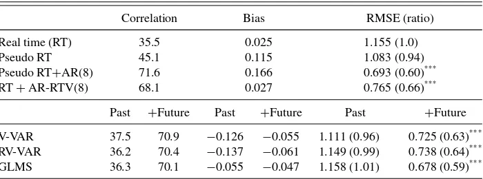
Table 2. Estimation of output gaps (HP filter)
Correlation Bias RMSE (ratio)
Real time (RT) 35.5 0.025 1.155 (1.0) Pseudo RT 45.1 0.115 1.083 (0.94) Pseudo RT+AR(8) 71.6 0.166 0.693 (0.60)∗ ∗ ∗ RT+AR-RTV(8) 68.1 0.027 0.765 (0.66)∗ ∗ ∗
Past +Future Past +Future Past +Future V-VAR 37.5 70.9 −0.126 −0.055 1.111 (0.96) 0.725 (0.63)∗ ∗ ∗ RV-VAR 36.2 70.4 −0.137 −0.061 1.149 (0.99) 0.738 (0.64)∗ ∗ ∗ GLMS 36.3 70.1 −0.055 −0.047 1.158 (1.01) 0.678 (0.59)∗ ∗ ∗
NOTE: The statistics are based on gap estimates for observationst=1985:Q2 to 2006:Q2. Pseudo RT uses 2010:Q1 vintage data; Pseudo RT+AR(8) augments this with forecasts of next 14 observations from an AR(8); RT+AR-RTV(8) is real time with forecasts of next 14 observations from AR-RTV(8). For V-VAR, RV-VAR, and GLMS,Pastindicates that past observations are replaced with model forecasts of the fully revised estimates of those observations;+Futureindicates past and future observations are replaced by forecasts of their fully revised values. The correlations are with the estimates obtained using all the data from the 2010:Q1 data vintage. Significant biases in the gap estimates at the 10%, 5%, and 1% levels are denoted by∗,∗ ∗, and∗ ∗ ∗after the bias estimate (where the tests use Newey-West standard errors). The same notation is used to denote statistically significant differences in MSE
relative to the real-time benchmark (one-sided tests).
increases to 71.6. The use of final data means this is infeasible, but real-time estimates with forecast augmentation using AR-RTV (as in Equation (6)) are nearly as highly correlated with the final estimates. The impact of the one-sided nature of the data available in a real-time setting outweighs data revision effects.
Table 2indicates that using backcasts has only a minor effect, and that forecasts of future observations are key to obtaining accurate gap estimates. Substituting estimates of post-revision data in Equation (9) has little effect. But whereas the V-VAR forecasts of past data are often statistically significantly more accurate than those of the no-change benchmark, as shown in Table 1, any improvements over AR-RTV for forecasting future observations are relatively modest. This is reflected in relatively small improvements in gap estimates from using the V-VAR forecasts relative to those of AR-RTV. The results for RV-VAR and GLMS are similar to the V-VAR: the V-VAR gives the highest correlation, GLMS the smallest RMSE, but differences between them are relatively minor. None of the sets of estimates are biased, and the RMSE ratios suggest that any forecast aug-mentation results in significantly more accurate real-time gap estimates on RMSE.
5. ESTIMATING THE INFLATION TREND AND GAP IN REAL TIME
We estimate trend inflation and the inflation gap as in the lit-erature by Stock and Watson (2007,2010; but see also Cogley, Primiceri, and Sargent2010). The deviation of inflation from trend (i.e., the inflation gap) is shown by Stock and Watson (2010) to have a stable relationship with the lagged unemploy-ment gap, where the inflation trend is interpreted as a measure of long-run expected inflation. Of interest is whether accurate es-timates of inflation trends and gaps can be obtained in real time, when the decomposition is applied to inflation data subject to revision, as opposed to the last vintage of data (the 2010:Q3 vintage in the case of Stock and Watson (2010)). We consider (a) whether data revisions have an important impact on the measurement of the inflation trend and cycle, and (b) whether forecasting data revisions using V-VAR models can improve the accuracy of real-time estimates of these quantities.
We begin by outlining the trend–gap decomposition. The observed inflation rate is decomposed into a trend and cycle using the Stock and Watson (2007) integrated moving aver-age (IMA(1,1)) model allowing for stochastic volatility. The IMA(1,1) is a reduced form representation of the following structural trend–cycle model:
πt =τt+ηt; E(ηt)=0, var(ηt)=ση,t2
τt =τt−1+εt; E(εt)=0, var(εt)=σε,t2 ,
cov(ηt, εt)=0, (11)
where πt is the quarter-on-quarter rate of inflation (at an
an-nualized rate);τt is the trend, which is a random walk driven
by a conditionally heteroscedastic disturbance,εt; andηt is the
cycle, which is also conditionally heteroscedastic. The trend is interpreted as a measure of the long-run expected inflation rate, and the filtered estimateτt|t is employed as the best forecast of
inflation using information up totby Stock and Watson (2010, Eqn. (1), p. 5). We measure the gap as the difference between current inflation and the filtered trend, that is, gapπ,t =πt−τt|t.
Croushore (2008) studied the nature of data revisions to core PCE inflation (the preferred measure of Stock and Watson2010), and found that revisions are predictable, matching our findings in Section3for the GDP deflator, suggesting that there might be scope for improving on real-time estimates. As a consequence, we consider both the GDP and PCE deflators. The estimate of the final gap gapπ,tand trendτt|tuse latest-vintage data (2010:Q1),
with an initial observation period of 1960:Q1. We used the same code as used by Stock and Watson (2010) that estimates the trend
τt|t using a Markov chain Monte Carlo algorithm, available on
Mark Watson’s webpage.
The real-time measures are obtained for all data vintagest+
1=1965:Q3 to 2006:Q3, with 1960:Q1 as the first observation: gaptπ,t+1=π
t+1
t −τ t+1
t|t ,
whereτtt|+t1is the estimate of trend using thet+1 data vintage to estimate Equation (11), that is, data{πit+1}fori=. . . , t−1, t. In contrast with the previous section, data revisions are the only source of disagreement between the final and the real-time measures because the inflation trend is computed with a one-sided filter.
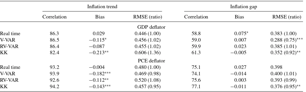
Table 3presents summary statistics for estimating inflation gaps and trends. Consider first the GDP deflator. In terms of estimating the inflation trend, the effect of using real-time data compared to the final-vintage data is fairly small. The correlation between the two measures is 86.3. The real-time GDP inflation gap estimates are less correlated with the final estimates, and there is a significant bias (at the 10% level) of 0.075. For the PCE deflator, the correlations of the real-time trend and gap estimates with the final are higher than for GDP inflation, and there is no significant bias. In the Supplementary Appendix, we show that the real-time inflation trend estimates perform poorly over specific periods (of 3–4 years duration) not withstanding these whole-period findings.
To attenuate the bias and reduce the variability of the real-time measures about the true values, we replace the data in thet+1 vintage that are still subject to the usual rounds of data revisions with forecasts of their post-revision values. Maintaining the assumption that the lastq−1 data points in vintaget+1 are not fully revised, these observations are replaced with forecast values
πtt−+q2+|t+21, πtt−+q3+|t+31, . . . , πtt+q|t+1.
The model in Equation (11) is then estimated using {πit+1},
i=. . . , t−1, t, whereπit+1=πit+1foriup tot−q+1, and πit+1=πii+q|t+1fori=t−q+2 tot.πii+q|t+1are forecasts of fully revised inflation rates.
Table 3 reports results for the V-VAR, RV-VAR, and KK models. The use of backcasts has little impact on the trend estimates, either in terms of correlation or MSE. However, the V-VAR backcasts improve real-time estimates of the GDP inflation gap by removing the bias and significantly reducing the RMSE. For both inflation measures, the KK model significantly reduces the real-time RMSE.
Clements and Galv ˜ao: Improving Real-Time Estimates of Output and Inflation Gaps 561
Table 3. Estimation of inflation trend and gap
Inflation trend Inflation gap
Correlation Bias RMSE (ratio) Correlation Bias RMSE (ratio)
GDP deflator
Real time 86.3 0.029 0.446 (1.00) 58.8 0.075∗ 0.383 (1.00) V-VAR 86.5 −0.115∗ 0.456 (1.02) 59.0 0.007 0.288 (0.75)∗∗∗ RV-VAR 86.4 −0.087 0.455 (1.02) 59.9 0.023 0.385 (1.01) KK 82.4 −0.213∗∗ 0.606 (1.36) 61.3 −0.005 0.352 (0.92)∗∗
PCE deflator
Real time 93.2 −0.004 0.480 (1.00) 75.1 0.027 0.398 V-VAR 93.9 −0.182∗∗∗ 0.469 (0.98) 74.1 −0.014 0.400 (1.01) RV-VAR 92.6 −0.112∗∗ 0.520 (1.08) 75.6 0.003 0.393 (0.99) KK 94.2 −0.143∗∗∗ 0.457 (0.95) 77.1 −0.011 0.376 (0.95)∗∗
NOTE: The statistics are based on trend and gap estimates for observationst=1985:Q2 to 2006:Q2. The correlations are with the estimates obtained using all the data from the 2010:Q1 data vintage. Significant biases in the gap estimates at the 10%, 5%, and 1% levels are denoted by∗,∗ ∗, and∗ ∗ ∗after the bias estimate (where the tests use Newey-West standard errors).
The same notation is used to denote statistically significant differences in MSE relative to the real-time benchmark (one-sided tests). KK is implemented with a diagonal K matrix.
6. CONCLUSIONS
We show that real-time estimates of output and inflation gaps can be improved by using past data vintages to predict revisions to past data and future observations. Because our forecasting models only use information on the variable in question, we are able to establish that improvements in the measurement of these key quantities are achievable simply by modeling the dy-namics of the data releases published by the statistical agency. Hence, we conclude that earlier-vintage data usefully supple-ments the latest-available vintage of data for real-time policy analysis. Information from other macroeconomic variables is also likely to play a role (see, e.g., Cunningham et al.2009), but we do not consider that issue. We regard the vintage-based VAR as a simple way of incorporating past-vintage information, because the unrestricted model can be estimated by OLS and the forecasts can be calculated using standard econometric soft-ware packages. We also consider alternative multiple-vintage models, such as the KK and the GLMS model, but the V-VAR forecasts were generally superior.
Our evaluation of the forecast performance of the different VAR models yields a number of insights. Revisions to past data are predictable—the VAR models improve upon the “no-change” benchmark forecasts. Moreover, data revisions to val-ues available two quarters after the observation period are pre-dictable, implying that the U.S. BEA annual revisions are in part predictable. Further extensions summarized in the Supplemen-tary Appendix suggest it is hard to improve upon the unrestricted VAR model by attempting to better approximate the seasonal nature of the release of data revisions.
The results of historical analyses of the output gap can be very misleading compared to what would have appeared to have been the case in real time. The same is not true to such an extent for filtered estimates of the inflation trend. The use of real-time data raises the variability of the measure of the inflation gap, but the trend is still a good measure of the long-run inflation expectations. However, if the task at hand requires an assessment of how far current inflation is from trend (the inflation “gap”), then using backcasts from multiple-vintage models improves the accuracy of inflation gap estimates in real time.
SUPPLEMENTARY MATERIALS
Appendix: A pdf file with descriptions of extensions to the forecasting models described in Section 2, tables evaluating the forecast performance of the additional models, and their value for estimating output gaps, inflation trends, and inflation gaps. It also includes additional figures.
ACKNOWLEDGMENTS
We gratefully acknowledge helpful comments and sugges-tions from seminar participants at Bath and Warwick, and from anonymous reviewers of this journal.
[Received May 2011. Revised May 2012.]
REFERENCES
Aruoba, S. B. (2008), “Data Revisions are Not Well-Behaved,”Journal of Money, Credit and Banking, 40, 319–340. [555]
Clark, T. E., and West, K. D. (2007), “Approximately Normal Tests for Equal Predictive Accuracy in Nested Models,”Journal of Econometrics, 138, 291– 311. [558]
Clements, M. P., and Galv˜ao, A. B. (2008), “Macroeconomic Forecasting With Mixed-Frequency Data: Forecasting Output Growth in the United States,” Journal of Business and Economic Statistics, 26, 546–554. [555] ——— (2012a), “Forecasting With Vector Autoregressive Models of Data
Vin-tages: US Output Growth and Inflation,”International Journal of Forecast-ing, doi:10.1016/j.ijforecast.2011.09.003. [556]
——— (2012b), “Real-Time Forecasting of Inflation and Output Growth With Autoregressive Models in the Presence of Data Revisions,”Journal of Ap-plied Econometrics, doi:10.1002/jae.2274. [557]
Clements, M. P., and Hendry, D. F. (2006), “Forecasting With Breaks,” in Handbook of Economic Forecasting(Vol. 1), eds. G. Elliott, C. Granger, and A. Timmermann, Amsterdam: Horth-Holland, pp. 605–657. [556] Cogley, T., Primiceri, G. E., and Sargent, T. J. (2010), “Inflation-Gap Persistence
in the US,”American Economic Journal: Macroeconomics, 2 (1), 43–69. [554,560]
Corradi, V., Fernandez, A., and Swanson, N. R. (2009), “Information in the Revision Process of Real-Time Datasets,”Journal of Business and Economic Statistics, 27, 455–467. [555]
Croushore, D. (2008),Revisions to PCE Inflation Measures: Implications for Monetary Policy, Working Paper No. 08-8, Philadelphia, PA: Research De-partment, Federal Reserve Bank of Philadelphia. [560]
——— (2011a), “Forecasting With Real-Time Data Vintages,” inThe Oxford Handbook of Economic Forecasting, eds. M. P. Clements and D. F. Hendry, New York: Oxford University Press, pp. 247–267. [555]
——— (2011b), “Frontiers of Real-Time Data Analysis,”Journal of Economic Literature, 49, 72–100. [555]
Croushore, D., and Stark, T. (2001), “A Real-Time Data Set for Macroe-conomists,”Journal of Econometrics, 105, 111–130. [557]
Cunningham, A., Eklund, J., Jeffery, C., Kapetanios, G., and Labhard, V. (2009), “A State Space Approach to Extracting the Signal From Uncertain Data,” Journal of Business & Economic Statistics, doi:10.1198/jbes.2009.08171. [555,561]
Elliott, G. (2006), “Forecasting With Trending Data,” inHandbook of Economic Forecasting (Vol. 1), eds. G. Elliott, C. Granger, and A. Timmermann, Amsterdam: Horth-Holland, pp. 555–604. [556]
Faust, J., Rogers, J. H., and Wright, J. H. (2003), “Exchange Rate Forecasting: The Errors We’ve Really Made,”Journal of International Economic Review, 60, 35–39. [555]
——— (2005), “News and Noise in G-7 GDP Announcements,”Journal of Money, Credit and Banking, 37 (3), 403–417. [555,558]
Fixler, D. J., and Grimm, B. T. (2005), “Reliability of the NIPA Estimates of U.S. Economic Activity,”Survey of Current Business, 85, 9–19. [555] ——— (2008), “The Reliability of the GDP and GDI Estimates,”Survey of
Current Business, 88, 16–32. [555]
Garratt, A., Lee, K., Mise, E., and Shields, K. (2008), “Real Time Representa-tions of the Output Gap,”Review of Economics and Statistics, 90, 792–804. [554,556,559]
—— (2009), “Real Time Representations of the UK Output Gap in the Presence of Model Uncertainty,”International Journal of Forecasting, 25, 81–102. [554]
Hecq, A., and Jacobs, J. P. A. M. (2009),On the VAR-VECM Representation of Real Time Data, Discussion paper, mimeo, Maastricht: Department of Quantitative Economics, University of Maastricht. [554]
Hodrick, R. J., and Prescott, E. (1997), “Post-War Business Cycles: An Empir-ical Investigation,”Journal of Money, Credit and Banking, 29, 1–16. [555] Howrey, E. P. (1978), “The Use of Preliminary Data in Economic Forecasting,”
Review of Economics and Statistics, 60, 193–201. [556]
Jacobs, J. P. A. M., and van Norden, S. (2011), “Modeling Data Revisions: Mea-surement Error and Dynamics of ‘True’ Values,”Journal of Econometrics, 161, 101–109. [555]
Kishor, N. K., and Koenig, E. F. (2011), “VAR Estimation and Forecasting When Data are Subject to Revision,”Journal of Business and Economic Statistics, 30, 181–190. [554,555,556]
Koenig, E. F., Dolmas, S., and Piger, J. (2003), “The Use and Abuse of Real-Time Data in Economic Forecasting,”Review of Economics and Statistics, 85 (3), 618–628. [557]
Kozicki, S., and Tinsley, P. A. (2005), “Permanent and Transitory Policy Shocks in an Empirical Macro Model With Asymmetric Information,”Journal of Economic Dynamics and Control, 29, 1985–2015. [554]
Landefeld, J. S., Seskin, E. P., and Fraumeni, B. M. (2008), “Taking the Pulse of the Economy,”Journal of Economic Perspectives, 22, 193–216. [555] Mankiw, N. G., and Shapiro, M. D. (1986), “News or Noise: An Analysis of
GNP Revisions,”Survey of Current Business, 66, 20–25. [555]
Orphanides, A. (2001), “Monetary Policy Rules Based on Real-Time Data,” American Economic Review, 91 (4), 964–985. [554]
Orphanides, A., and van Norden, S. (2002), “The Unreliability of Output Gap Estimates in Real Time,”Review of Economics and Statistics, 84, 569–583. [554,559]
Patterson, K. D. (2003), “Exploiting Information in Vintages of Time-Series Data,”International Journal of Forecasting, 19, 177–197. [556]
Sargent, T. J. (1989), “Two Models of Measurements and the Investment Ac-celerator,”Journal of Political Economy, 97, 251–287. [556]
Sims, C. A. (1980), “Macroeconomics and Reality,”Econometrica, 48, 1–48. [554]
Stock, J. H., and Watson, M. W. (2007), “Why has U.S. Inflation Become Harder to Forecast?,”Journal of Money, Credit and Banking, 39 (S1), 3– 33. [554,555,560]
——— (2010),Modelling Inflation After the Crisis, NBER Working Paper Series, 16488, Cambridge, MA: National Bureau of Economic Research. [554,555,560]
Watson, M. W. (2007), “How Accurate are Real-Time Estimates of Output Trends and Gaps?,”Federal Reserve Bank of Richmond Economic Quarterly, 93, 143–161. [559]