Full Terms & Conditions of access and use can be found at
http://www.tandfonline.com/action/journalInformation?journalCode=ubes20
Download by: [Universitas Maritim Raja Ali Haji] Date: 13 January 2016, At: 00:39
Journal of Business & Economic Statistics
ISSN: 0735-0015 (Print) 1537-2707 (Online) Journal homepage: http://www.tandfonline.com/loi/ubes20
Robust Stationarity Tests in Seasonal Time Series
Processes
A. M Robert Taylor
To cite this article: A. M Robert Taylor (2003) Robust Stationarity Tests in Seasonal
Time Series Processes, Journal of Business & Economic Statistics, 21:1, 156-163, DOI: 10.1198/073500102288618856
To link to this article: http://dx.doi.org/10.1198/073500102288618856
Published online: 01 Jan 2012.
Submit your article to this journal
Article views: 45
Robust Stationarity Tests in Seasonal
Time Series Processes
A. M. Robert
Taylor
Department of Economics, University of Birmingham, Birmingham B15 2TT, U.K. (r.taylor@bham.ac.uk)
This article builds on the existing literature on (stationarity) tests of the null hypothesis of deterministic seasonality in a univariate time series process against the alternative of unit root behavior at some or all of the zero and seasonal frequencies. This article considers the case where, in testing for unit roots at some proper subset of the zero and seasonal frequencies, there are unattended unit roots among the remaining frequencies. Monte Carlo results are presented that demonstrate that in this case, the station-arity tests tend to distort below nominal size under the null and display an associated (often very large) loss of power under the alternative. A modication to the existing tests, based on data preltering, that eliminates the problem asymptotically is suggested. Monte Carlo evidence suggests that this procedure works well in practice, even at relatively small sample sizes. Applications of the robustied statistics to various seasonally unadjusted time series measures of U.K. consumers’ expenditure are considered; these yield considerably more evidence of seasonal unit roots than do the existing stationarity tests.
KEY WORDS: Preltering; Seasonality; Stationarity tests; Unattended unit roots.
1. INTRODUCTION
In a recent article, Canova and Hansen (1995) (hereafter CH) developed score-based tests for the null hypothesis of deterministic seasonality against the alternative of unit roots at some or all of the seasonal, but not zero, frequencies. Their tests are similar in spirit to the tests against a zero frequency unit root developed by Kwiatkowski, Phillips, Schmidt, and Shin (1992) (hereafter KPSS) and are derived from the gen-eral theory on parameter stability testing of Hansen (1992). These statistics retain pivotal Cramer–von Mises limit distribu-tions even under weakly dependent and heterogeneous errors via the use of a nonparametric heteroscedasticity and autocor-relation consistent (HAC) covariance matrix estimator. Under much stronger assumptions on the errors, Caner (1998) devel-oped variants of the CH tests that replace the nonparametric HAC estimator with a parametric correction, developed along similar lines to that used in testing against zero frequency unit roots by Leybourne and McCabe (1994). Taylor (2003) amal-gamated the aforementioned seasonal and nonseasonal fre-quency material to develop tests against seasonaland/orzero frequency unit roots. A brief review of this literature is given in Section 2.
In this article attention is focused on an issue originally highlighted by Hylleberg (1995). Discussing the CH tests, Hylleberg provided simulation evidence to show that when testing for a unit root at a certain seasonal frequency, the size and power properties of this test can be adversely affected if there are unit roots at other seasonal frequencies of the data, what he termed “unattended unit roots.” Section 3 gives exten-sive Monte Carlo evidence that further supports this position. The results demonstrate that inferences at one frequency will be affected as to whether, and at what strength, unit roots occur at unattended frequencies. This issue has also been partly recognized by CH, who argued that when testing against purely seasonal unit roots, one should rst-difference the data before analysis. However, as the simulation evidence presented in Section 3 and by Hylleberg (1995) makes clear, unattended
seasonal frequency unit roots have qualitatively similar effects to unattended zero frequency unit roots.
In Section 4 a practical solution to this problem is pro-posed. The suggestion is made that when testing for a unit root at a particular frequency, one should rst transform the data by applying a differencing lter (prelter) that reduces the order of integration at each of the remaining (unattended) frequencies by one. It is demonstrated that such preltering renders the limiting null distributions of the resulting stationar-ity test statistics invariant as to whether or not unattended unit roots are actually present. Monte Carlo evidence is provided suggesting that such preltering can yield considerable power gains in nite samples relative to the case where preltering is not conducted. Moreover, the nite-sample power of the tests based on such preltered data appears largely unaffected by whether or not these unattended unit roots exist in the data. Section 5 presents empirical applications to a variety of mea-sures of U.K. quarterly consumption. Section 6 concludes. All proofs are contained in an Appendix.
2. TESTING AGAINST UNIT ROOTS IN SEASONAL PROCESSES
Consider the scalar time series process8yt9, observed with constant seasonal periodicityd, satisfying the data-generating process (DGP),
ytDZ
0
ttÄCZ
0
tÃtC…t1 tD11: : : 1T (1)
and
ÃtDÃtƒ1Cut1 ut¹IID401G51 tD11: : : 1T 0 (2)
©2003 American Statistical Association Journal of Business & Economic Statistics January 2003, Vol. 21, No. 1 DOI 10.1198/073500102288618856
156
Taylor: Stationarity in Seasonal Time Series Processes 157
In (1),ZtD4z
01 tz011 t¢ ¢ ¢z0d=21t5
0,
¢denoting the integer part
of its argument, is ad-vector of spectrally identied indicator variables; that is,z
assume that the error process …t satises the strong mixing conditions laid out in Assumption 1 of Taylor (2003).
The matrixGDdiag4ˆ11 : : : 1 ˆd5of (2) contains the hyper-parameters associated with each element ofÃt. Ifˆk>0, then thekth element ofÃt follows a random walk, whereas ifˆk1 tD 0, thenƒk1 treduces to a xed constant for allt. Consequently, from (1)–(2),ˆ1>0 yields a unit root at the zero spectral
fre-quency,—²0;ˆd>0,d even, yields a unit root at frequency
(also termed the Nyquist frequency),—², whereas a pair of complex conjugate unit roots at thekth harmonic seasonal frequency pair,4—k12ƒ—k51 —kD2k=d,k2811 : : : 1 dü9,
is obtained underˆ2kDˆ2kC1>0. Unit roots occur at all of
the zero and seasonal frequencies ifˆk>01 kD11 : : : 1 d. To test the null hypothesis of deterministic seasonality against unit root behavior at certain (possibly all) of the spec-tral frequencies,—kD2k=d1 kD01 : : : 1 dƒ1, dene the full column rankdc11µcµd, selection matrixC
1, comprising
thec columns ofI
d, thedd identity matrix, which selects the c elements of Ãt to test for random walk behavior. The associatedd4dƒc5 matrix C
2 is also dened to comprise
thedƒccolumns ofI
d notinC1. It will prove convenient in
what follows to rewrite (1) as
ytD test, consider the hypothesis structure
H02È1D0 (4)
2È contains all elements of È not included in
È1. The notation È1>0 is used to indicate that ˆ
11 j ¶0 for eachj with inequality for at least onej, that is, a one-sided alternative. UnderH0of (4) ÃtDÃ, for allt, so that (1)–(2),
a strong mixing process displaying deterministic seasonal behavior with a seasonally varying linear trend. In contrast, underH1 of (5),8yt9has unit root(s) at the frequencies deter-mined by the form ofC
1 and byÈ1.
As demonstrated by Taylor (2003), a consistent test forH0
of (4) againstH1 of (5), is dened by the critical region
¬DTƒ2tr
where ` is a suitably chosen (positive) constant, “tr” denotes the trace operator, …Ot, tD11 : : : 1 T, are the ordi-nary least squares (OLS) residuals from estimating the null model (7). Following CH, the HAC estimator of
ì1 ² limT!ˆTƒ1E44PTtD1Z11 t…t54
where the autocovariance estimator bâ4j5 DTƒ1PT tDjC1…Ot
Z
11 t…OtƒjZ011 tƒj, bâ4ƒj5Dbâ4j5
0, j ¶0. Suitable choices for
the kernel functionk4¢5 have been given by Priestley (1981,
pp. 446–447) and Andrews (1991, p. 821), while setting the bandwidth parameterST such thatST ! ˆandST=T1=2!0
(8) the locally best invariant test ofH0 of (4) againstH1 of
(5) in the directionˆ111D¢ ¢ ¢Dˆ11 c>0, provided thatÈ2D0;
(cf. Nyblom 1989, eq. 4.2, p. 228).
Remark 2. If it is known that ÄD0 in (1), then the test
statistic¬ should be constructed from the OLS residuals…Oü
t from the regression ofyt onZ
t,tD11 : : : 1 T. Similarly, if it
Remark 3. FordD1, the statistic¬constructed from the OLS residuals…Ot and …Oüt coincides with‡’ and‡Œ of KPSS [eqs. (15), p. 167 and (13), p. 165]. Ford >1 and choosing
C
1D41101 : : : 105
0,¬ is a KPSS-type test statistic, differing
from the KPSS statistic only by the presence of the seasonal deterministic regressors in the estimated null regression (7).
Remark 4. If the statistic ¬ is constructed using the …Oü
t residuals, then (a) for d even, ¬ will coincide with the ¬
statistic of CH [eq. (17), p. 6] on choosingC
1D400: : :15
1to comprise all but the rst column
ofI
d renders¬equivalent to the¬f statistic of CH [eq. (15), p. 5].
The following theorem demonstrates that, provided that the maintained hypothesisHM of (6) holds, the score-based test statistic¬of (8) has a pivotal limiting null distribution
belong-ing to a well-known family of distributions.
Theorem 1. Let yt be generated by (1)–(2) under H0 of
where “)” denotes weak convergence andGc4r5is a vector
standard second-order Brownian bridge of dimensionc.
Corollary 1. If ¬ is derived from the OLS residuals …Oü
t, as in Remark 2, then its limiting distribution is given by (10), on replacing Gc4r 5 with Bc4r 5, a vector standard Brownian
bridge of dimensionc. This result also holds when using the OLS residuals…Oüü
t , provided that the vector41 01 : : : 105
0does
not lie in the column space ofC
1. Where the rst column, say,
ofC
1is the vector41 01 : : : 105
0
, the limiting distribution of¬
in this case is given by (10) but replacingG
c4r 5 byHc4r 5, a
c-dimensional limit process whose rst element is a standard second-order Brownian bridge process and remaining cƒ1 elements are standard Brownian bridge processes.
Remark 5. The foregoing limiting distributions belong to the family of generalized Cramer–von Mises distributions (see Harvey 2001 for further discussion). Selected critical values from these distributions have been provided by Taylor (2003) and CH.
Theorem 1 was derived under the assumptions thatÈ2D0
[i.e., the maintained hypothesisHM of (6)] and thatì1is
pos-itive denite. The rst assumption ensures that poles do not exist at the spectral frequencies not identied byC
1; the
con-sequences of this assumption failing to hold are explored in the next section. The second assumption rules out zeros in the spectrum of 8…t9 at any of the frequencies identied by the selection matrix C
1. There is, however, no requirement that
the spectral density of8…t9 be nonzero at those spectral fre-quencies identied byC
2, and it is this result that will prove
pivotal in the ability to develop robustied statistics in Section 4 that retain the limiting null distributions given earlier, irre-spective ofÈ2. At this point, it is worth noting that paramet-ric stationarity tests of the type considered by Leybourne and McCabe (1994) and Caner (1998), where the nonparametric HAC estimator in (8) is replaced by a parametric estimator, can also be used to test againstH1of (5). However, such tests
require the much stronger assumption that8…t9 of (1) admits a nite-order stationary AR representation. Because processes with spectral zeros do not have AR representations, parametric variants of the robust statistics that are subsequently developed in Section 4 would not be viable. Consequently, parametric stationarity tests are not considered in this article.
3. UNATTENDED UNIT ROOTS
Hylleberg (1995) highlighted a serious shortcoming with the tests of Section 2, which he terms the problem of unattended unit roots. This problem translates into how one chooses the matrix C
1 in practice. Thus far, it has been assumed thatC1
is chosen such that the maintained hypothesis,HM of (6), is not violated. However, in practice, one cannot know which of the spectral frequencies admits a unit root. If one did know this, then one would have no need for unit root testing. To that end, suppose now thatC
1is chosen is such a way that the
maintained hypothesis,HM, is violated; that is,È2 is a xed 4dƒc5-vector of constants such thatÈ2>0. In this case, the
following theorem may be stated.
Theorem 2. Let yt be generated by (1)–(2) with È2>0.
Then, underH0 of (4),¬of (8) isOp44TST5ƒ15.
Given the results of Theorem 2, one would anticipate that in the presence of unattended unit roots (i.e., cases whereHM is violated), a test based on¬of (8) will be undersized
(increas-ingly so as the sample size increases) with an associated loss of power under H1 of (5), the latter due to the usual
nite-sample trade-off between type I and type II errors in hypoth-esis testing. To quantify these effects in nite-samples, the results from a Monte Carlo experiment conducted using the quarterly (dD4) DGP are presented:
ytDZ0
tÃtC…t1 tD11 : : : 1 T (11)
and
ÃtDÃtƒ1Cut1 tD11 : : : 1 T 1 (12)
where Zt D 411cos4t=251sin4t=251 4ƒ15t50 and Ãt ²
4ƒ11t1 : : : 1 ƒ41t50 with Ã0D0. The error processes was
gen-erated according to …t ¹IN40115 and u
t¹ IN401G5, inde-pendent of …t, with GDdiag4ˆ11 ˆ21 ˆ21 ˆ35. Here 8…t9 has been generated as a serially uncorrelated sequence to show the effects of unattended unit roots, uncontaminated by issues arising from serial correlation in the errors. The latter is already well documented for the tests of Section 2 (see KPSS pp. 169–173; Hylleberg 1995; CH, pp. 8–12; Caner 1998). In the results reported here the sample size varies among T 2
840110012009 and the signal-to-noise ratios (hyperparame-ters) vary among certain combinations ofˆj2801 011 021 05119,
jD11 : : : 13. Other values for these design parameters were also investigated. These results, available on request, qualita-tively add nothing to the reported results. Under (11)–(12), the stationary (unit root) hypothesis holds at the zero, Nyquist, and seasonal harmonic frequencies when ˆ1D0 (ˆ1>0), ˆ3D0
(ˆ3>0), andˆ2D0 (ˆ2>0).
To implement the tests, an appropriate estimatorìb1 must be selected for the long-run covariance matrix ì1. There-fore, both a kernel functionk4¢5 and a bandwidth parameter
ST must be chosen. The results, reported in Tables 1 and 2, are for the Bartlett kernel with ST D4 if T D50, ST D6 if T D100, and ST D8 if T D200. Other values of ST were also explored; these results are not reported because they do not add anything to the present discussion, they simply reect the well-known trade-off between size and power (see KPSS pp. 169–173; Hylleberg 1995; CH pp. 10–11). All tests were run at the nominal .05 level, using the asymptotic critical val-ues from page 5 of CH. All experiments in this section were programmed using the RNDN function of GAUSS 3.1, in each case using 50,000 replications.
Table 1 reports the nite-sample behavior of the tests based on the ¬
0, ¬, ¬=2, and ¬0: : :2 statistics; that is, (8)
under C
1D41 0 0 05
0, C
1D40 0 0 15
0, C
1D40 I205
0, and
C
1DI4. Recall that the KPSS-type statistic¬0is used to test
H0112 ˆ1D0 againstH1112 ˆ1>0, withˆ2Dˆ3D0 maintained.
Similarly, the CH statistics¬
and¬ =2are used to testH0132
ˆ3D0 againstH1132 ˆ3>0, withˆ1Dˆ2D0 maintained and
H0122 ˆ2D0 againstH1122 ˆ2>0, withˆ1Dˆ3D0 maintained.
The joint statistic¬
0: : :2 is used to testH02 ˆ1D¢ ¢ ¢Dˆ3D0
versus H12[ 3
jD14ˆj>05. Each test statistic was constructed
Taylor: Stationarity in Seasonal Time Series Processes 159
Table 1. Size and Power of Stability Tests: No Data Pre’ltering
¬0 ¬ ¬ =2 ¬0: : :2
ˆ1 ˆ3 ˆ2 40 100 200 40 100 200 40 100 200 40 100 200
01 0 0 019 050 073 003 004 004 001 002 003 010 036 060
02 0 0 037 066 082 003 003 003 001 002 002 020 052 069
05 0 0 056 074 086 002 001 001 000 001 001 035 058 069 100 0 0 061 075 086 001 000 000 000 000 000 034 055 066 0 01 0 003 004 004 019 050 072 001 002 003 010 036 060 0 02 0 003 003 003 037 066 082 001 002 002 020 053 070 0 05 0 002 001 001 056 074 086 000 000 001 034 058 069 0 100 0 001 000 000 060 076 086 000 000 000 034 055 066 0 0 01 003 004 004 003 004 004 014 055 084 010 045 079 0 0 02 003 003 003 003 003 003 036 080 094 024 073 091 0 0 05 001 001 001 001 001 001 070 091 097 055 086 094 0 0 100 001 000 000 001 000 000 079 093 098 066 087 094
01 01 01 013 045 069 013 045 069 006 044 080 021 082 097
01 02 02 012 042 066 029 062 080 014 072 092 043 094 1000
01 05 05 006 027 053 047 070 082 040 085 094 074 098 1000
01 100 100 001 010 030 050 071 083 051 087 096 081 098 1000
02 01 02 030 062 079 011 042 066 014 072 092 043 094 1000
05 01 05 047 070 082 005 027 053 041 085 095 074 098 1000 100 01 100 050 071 084 001 010 030 051 087 096 081 098 1000
02 02 01 030 062 079 030 062 079 004 037 077 040 091 099
05 05 01 048 070 083 047 070 083 001 016 055 065 093 099 100 100 01 052 072 084 052 071 084 000 003 024 070 091 098
from the OLS residuals…Oüt, obtained from estimating the null model,
ytDZ
0
tÃC…t1 tD11 : : : 1 T 0 (13)
Also considered were the corresponding tests based on statis-tics constructed from the OLS residuals…Ot or…Oüüt ; see Remark 2. As would be expected, the behavior of the test based on the¬
0statistic in both such cases relative to the case reported
was very similar to that of the test based on ‡OŒ relative to that based on ‡O’ reported by KPSS (Table 4, p. 172). That is, for alternatives close to the null, the test based on the¬
0
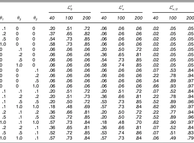
Table 2. Size and Power of Stability Tests: Pre’ltered Data
¬f
0 ¬f ¬f =2
ˆ1 ˆ3 ˆ2 40 100 200 40 100 200 40 100 200
01 0 0 020 051 072 006 006 006 002 005 005
02 0 0 037 065 082 006 006 006 002 005 005
05 0 0 054 073 085 006 006 006 002 005 005 100 0 0 058 073 085 006 006 006 002 005 005 0 01 0 006 006 006 020 050 072 002 005 005 0 02 0 006 006 006 036 065 081 002 005 005 0 05 0 006 006 006 054 073 085 002 005 005 0 100 0 006 006 006 058 074 085 002 005 005 0 0 01 006 006 006 006 006 006 007 053 084 0 0 02 006 006 006 006 006 006 022 078 094 0 0 05 006 006 006 006 006 006 054 089 097 0 0 100 006 006 006 006 006 006 066 093 097
01 01 01 020 051 072 020 051 072 007 052 084
01 02 02 020 051 073 036 066 081 022 078 094
01 05 05 020 050 072 053 073 085 052 089 096
01 100 100 018 048 069 057 073 084 062 090 097
02 01 02 036 066 081 020 050 072 022 077 094
05 01 05 052 072 085 020 050 072 052 089 096 100 01 100 057 073 084 018 048 070 062 090 097
02 02 01 036 065 081 036 066 081 007 052 084
05 05 01 052 072 085 053 074 086 007 051 083 100 100 01 057 073 084 057 073 084 006 049 079
statistic formed from the…Otüresiduals is somewhat more pow-erful that based on the¬
0the statistic constructed from either
the…Ot or…Otüü residuals, with the pattern tending to reverse for alternatives further from the null. Similar patterns are seen between tests based on the¬ and¬ =
2statistics when formed
from either the …Oü
t or …O
üü
t residuals vis-à-vis the …Ot residu-als. These patterns were replicated in the preltered tests of Table 2. Full details are available on request.
Also considered were the parametric stationarity tests dis-cussed at the end of Section 2 using the data-dependent lag selection method outlined by Caner (1998). But the results were qualitatively no different from those reported in Table 1
for the nonparametric tests and hence are not reported here. Again, full details may be obtained on request.
Consider the rst 12 rows of Table 1, all cases in which only one of theˆj,jD11 : : : 13, parameters deviates from 0. UnderH111,H113, andH112the tests based on the¬0,¬, and
¬=
2 statistics are seen to demonstrate power that, under a
xed alternative, increases with T, reecting the consistency of the tests. For a xed sample size, the power of the tests also tends to increase as the correspondingˆj increases, although some exceptions exist. For example, for T D200, there is no increase in the power of the test based on the KPSS-type¬
0
statistic for ˆ1D05, ˆ2Dˆ3D0 vis-à-vis ˆ1D1, ˆ2Dˆ3D
0. This nonmonotonicity property was also documented by KPSS (p. 173) for tests using their‡OŒ and‡O’ statistics, and is reected in the joint test based on¬
0: : :2. In cases where the
maintained hypothesis (that there are no unit roots present at frequenciesnot under test) is violated, the tests demonstrate rejection frequencies that fall below the nominal size level. As a representative example, whenˆ1D05, ˆ2Dˆ3D0, the test
based on¬0displays a power of .56 forT D40, increasing to .86 forT D200. In contrast, the rejection frequencies for the CH tests based on the¬ and¬=
2 statistics in this case are
.02 and 0 forT D40 and .01 and .01 forTD200.
Two other points merit attention. First, on interchanging the values ofˆ1withˆ3, the patterns seen for the test based on the
¬
0 statistic are almost identical to those seen for the CH test
based on the¬
statistic. Second, underH111,H113, andH112
the tests based on the¬
0,¬, and¬=2 statistics all display
superior power to the joint frequency test based on¬
0: : :2. To
illustrate, in the case considered earlier where ˆ1D05, ˆ2D
ˆ3D0, the test based on ¬0: : :2 displays power of .35 for
T D40 and .69 atT D200, in each case somewhat below the power of the KPSS-type test based on the¬
0statistic.
The nal 10 rows of Table 1 highlight cases where more than one of theˆj parameters moves away from 0. In such cases, one would hope that the tests based on the¬
0,¬, and
¬=
2 statistics will be able to identify frequencies at which
there are unit roots just as effectively as in cases where only one parameter moves away from 0. However, as is clearly demonstrated in Table 1, this is not the case. The problem stems from the “undersizing” phenomenon of the tests in the presence of unattended unit roots, noted earlier. As a repre-sentative example, forT D100 andˆ1D01, the test based on
¬
0 rejects the null only 10% of the time when ˆ2Dˆ3D1,
compared to 50% (45%) of the time whenˆ2Dˆ3D04015. In
contrast, the joint frequency test based on¬
0: : :2 displays an
increase in power from .36 to .98 forˆ1D01 withˆ2Dˆ3D0
vis-à-visˆ2Dˆ3D1. Similar patterns are seen in the seasonal frequency tests based on the¬ and¬=
2statistics. For
exam-ple, forTD100 and ˆ2D01, the test based on¬ =2 displays
a rejection frequency of .55 whenˆ1Dˆ3D0, but displays a
rejection frequencybelowthe nominal level whenˆ1Dˆ3D1.
Although the problem appears most pronounced in smaller samples, because the tests have lower power against a xed alternative here, it does not vanish as the sample size increases. For example, whenTD200, the test based on the¬0 statistic shows a rejection rate of .73 forˆ1D01,ˆ2Dˆ3D0, reducing
to .30 forˆ1D01,ˆ2Dˆ3D1.
So it is, for example, quite possible for a particular outcome of the joint test to be signicant while all of the subset fre-quency tests have insignicant outcomes. Put simply, the infer-ences at one frequency will be affected as to whether, and with what signal-to-noise ratios, unit roots occur at other (unat-tended) frequencies. As a leading example, macroeconomic time series data often appear to have their greatest spectral mass at the zero frequency. Tests against seasonal frequency unit roots are therefore likely to be biased toward nonrejection in practice.
4. ROBUSTIFIED TESTS
The problem of unattended unit roots, discussed in Section 3, can be avoided by considering only the joint test against unit roots at the zero and seasonal frequencies; that is, settingC
1DId in constructing¬. BecauseHM cannot be vio-lated in the case of the joint test, this will be more powerful than the individual frequency tests where unit roots exist at more than one of the zero and/or seasonal frequencies, as was conrmed by the Monte Carlo results reported in Section 3. There are two main drawbacks to this solution, however. First, if the maintained hypothesisHM of (6) does hold, then indi-vidual frequency tests will dominate the joint test on power; see Remark 1. This was seen very clearly in the Monte Carlo results reported in Section 3. Second, a rejection by the joint frequency test reveals nothing about which specic elements of à of (2) are rejecting the stability hypothesis, indicating merely that the hypothesis thatÃis stable cannot be accepted. In practice, the applied worker will want guidance as to which frequency (or frequencies) are rejecting the stability hypothe-sis. However, as was discussed at the end of Section 3, this is likely to be confounded if the data contain unit roots at more than one of the zero and/or seasonal frequencies.
Consider now the differencing lter,F 4L5, whereLdenotes the usual lag operator such thatLky
t²ytƒk, which reduces by one the order of integration at all of the spectral frequencies corresponding to those elements ofÃt chosen byC
2. The order
of this lter is denoted by f. The relevant prelter for the
¬
Now considerprelteringthe process8yt9generated by (1)– (2) by F 4L5, so that Although the term Z0
1tÃ1t of (2) has been transformed to
F 4L5Z0
1tÃ1t in (14), those regressors in Z1t identied with a particular spectral frequency span an space identical to the cor-responding regressors in F 4L5Z
1t. Consequently,F 4L5Z
0
1tÃ1t may be treated exactly as if it wereZ0
1tÃ1t in constructing tests ofH0of (4) againstH1 of (5).
It is clear that the disturbance term …ü
t of (14) contains a moving average of order f in …t. Moreover, 8…üt9 is strictly
Taylor: Stationarity in Seasonal Time Series Processes 161
noninvertible at those spectral frequencies associated with any zero elements in È2 but not at those frequencies associated withZ
1t; (see Harvey 1989, pp. 54–70 for rigorous discussion on this point). Consequently, provided thatì1is positive
de-nite,ìü1²limT!ˆTƒ1E44PTtDfC1Z1t…
be positive denite, and so forming the statistic¬of (8) from
the preltered dataF 4L5yt, rather than fromyt, will retain the pivotal limiting null distributions of Theorem 1 and Corol-lary 1, irrespective of whether or notHM of (6) holds. This result is formalized in the following theorem.
Theorem 3. Consider the statistic
¬fDTƒ2Trace generated by (1)–(2) with ì1 positive denite. Then, under
H0 of (4), the limiting distribution of¬
f is given by the right member of (10), regardless of the value of È2. The results stated in Corollary 1 for¬of (8) also apply to¬f.
Table 2 explores the nite-sample properties of the sta-tionarity tests based on the statistics from the preltered data under the same experimental design as was used for the results reported in Table 1. To be precise, ¬f
0, the
pre-ltered version of the ¬
0 statistic, is constructed using the
OLS residuals from the regression of41CLCL2CL35y
t on
Z
t, tD41 : : : 1 T, whereas ¬f, the preltered version of the
¬ statistic, is constructed using the residuals from the
regres-sion of41ƒLCL2ƒL35y
t onZt,tD41 : : : 1 T. Finally,¬ f =2,
the preltered version of the ¬ =
2 statistic, is formed from
the OLS residuals from the regression of 41ƒL25y
t on Zt,
tD31 : : : 1 T. The results in Table 2 indicate that the tests based on the statistics formed from the preltered data display relatively similar rejection frequencies, regardless of whether or not the maintained hypothesis is violated, to the standard tests under the maintained hypothesis reported in Table 1. Thus, contrast to the standard tests, unattended unit roots seem to have little effect on the behavior of the preltered tests, as predicted by the limiting distribution theory. For example, for T D100 and ˆ1D1, ˆ2Dˆ3D0, the tests based on the¬ and¬ =
2 statistics both display a rejection rate of 0, whereas
the corresponding tests based on the¬f and¬
f
=2statistics are
approximately on the nominal size. Variations from the nom-inal level are merely small-sample effects, attributable to the efciency of theìbü1 estimator in accommodating the induced moving average behavior in…üt. The only signicant examples of this occur for the test based on the¬f
=2 statistic atT D40,
and this should be borne in mind when assessing the power of that test for T D40. As a second example, for T D100 andˆ2D01,ˆ1Dˆ3D05, from Table 1, the tests based on the
¬
0¬,¬=2, and¬0: : :2statistics display rejection frequencies
of .70, .70, .16, and .93. In contrast, the power of test based on the¬ =
2 statistic whenˆ1Dˆ3D0 is .55. However, looking
at the corresponding entries in Table 2, it is seen that the tests based on the¬f
0 and¬
f
statistics both show a small increase
in power over the corresponding tests for the unltered case, whereas the test based on the ¬f
=2 statistic displays a
rejec-tion frequency of around .52 irrespective ofˆ1andˆ3, which
is comparable with the power of the test based on¬ =
2when
the maintained hypothesisˆ1Dˆ3D0 holds. Similar examples
occur throughout Table 2.
Given the results in Tables 1 and 2, the conclusions here are straightforward. Routine preltering of (potential) unit roots at all of the zero and/or seasonal frequencies not directly under test from the data is recommended before the stationarity tests are computed. Unlike the standard tests, the behavior of the preltered tests is ambivalent as to whether or not such unit roots exist in the data. Thus this appears to be a very use-ful method of maintaining poweruse-ful tests against unit roots at some proper subset of the zero and/or seasonal frequen-cies where there are unattended unit roots at one or more of the residual frequencies. This strategy seems particularly important in cases where the practitioner is able to reject the null hypothesis of stability of the entire vectorà of (13) and wishes to establish those of the zero and seasonal frequencies at which the stability hypothesis appears unfounded. As has been shown, failure to do so makes it considerably less likely that the practitioner will be able to achieve this goal.
5. EMPIRICAL APPLICATIONS
As a practical illustration of the tests developed in arti-cle, they are applied to a variety of measures of U.K. con-sumers’ expenditures. Specically, the series considered are real quarterly, seasonally unadjusted consumers’ expenditure on tobacco, beer, household goods, alcohol and tobacco, cloth-ing and footwear, total durable goods, do-it-yourself (DIY) goods, dairy products, foods (vegetables), foods (meat and bacon), and catering. The rst four series are observed for the sample period 1955.1–1996.1; the next two series, for 1955.1–1995.1; and the nal ve series for, 1963.1–1996.1. All datasets were extracted from the U.K. ONS macroeco-nomic database.
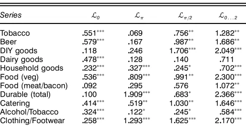
Table 3 reports the application of the ¬
0, ¬, ¬=2, and
¬
0: : :2 statistics of Section 3, for d D4 to the logarithm of
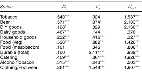
each of the aforementioned consumption series. The values of the preltered versions of these statistics,¬f
0, ¬f,¬ f =2, and
¬f
0: : :2, calculated as detailed in Section 4, are presented in
Table 3. Stability Statistics for U.K. Consumption Data: No Data Pre’ltering
Table 4. Stability Statistics for U.K. Consumption Data: Pre’ltered Data
Household goods 0232üüü
0416üüü
Table 4. For all test statistics reported in this section, signif-icant outcomes at the .10, .05, and .01 levels are agged by
ü
,üü, and üüü. The covariance matrix estimators ìb1 and ìbü1, used the Newey and West (1987) procedure with the Bartlett window and with lag truncationST D6 for the rst six series listed earlier and ST D5 for the last ve series. In the case of household goods and alcohol/tobacco, the estimated null regression (7) was specied according to the leading case, that is seasonal intercepts and seasonal trends were used, whereas for all other variables considered, seasonal intercepts and a linear trend were deemed appropriate.
The results in Tables 3 and 4 appear to be in concert with the Monte Carlo results reported in Sections 3 and 4. The sea-sonal frequency unit root tests using the preltered ¬f
and
¬f=
2 statistics (see Table 4) provide considerably more
evi-dence againstH0of (4) than do the corresponding tests using
the¬
and¬=2statistics formed from the untransformed data
(see Table 3). Among the most notable illustrations of this result are seen between the outcomes of both the¬ and¬f
and the¬
=2 and¬
f
=2 statistics for the alcohol and tobacco
series and between the¬
=2 and¬
f
=2statistics for the
house-hold series. In the rst of these examples, using untransformed data, the values of the¬
0 and¬0: : :2 test statistics both give
sufcient evidence to rejectH0 at the .01 signicance level,
whereas the outcomes of the¬ and¬ =
2statistics are
signif-icant only at the .10 level. However, in the preltered case, the outcomes of the¬f
0,¬
f , and¬
f
=2statistics are all signicant
at the .01 level. In the second example, using untransformed data, the¬
0,¬, and¬0: : :2 statistics are all signicant at the
.01 level, whereas the¬=
2 statistic is signicant at only the
.10 level. In contrast, the outcome of the preltered¬f
=2 test
statistic is signicant at the .01 level. Many similar examples can be seen across Tables 3 and 4. In contrast to the seasonal frequencies, a comparison of the results in Tables 3 and 4 shows that in most cases, the inferences drawn from the tests based on the¬f
0 and ¬0 statistics will coincide for a given
level. Given the apparent strength of the zero frequency unit root in most of these series, this is to be expected in light of the simulation results from Sections 3 and 4. However, in the case of the DIY goods series, the outcome of the preltered
¬f
0 test statistic allows rejection ofH0at the .10 level, whereas
that of¬
0 does not.
A further example of particular interest is provided by the foods (meat and bacon) series. Here H0 of (4) is rejected
at the .05 level by the joint test based on ¬
0: : :2. However,
using the untransformed data, the outcomes of the ¬
0, ¬, and¬
=2test statistics are of little use in identifying at which
of the zero and/or seasonal frequencies the stability hypothe-sis appears unfounded, with none proving signicant, even at the .10 level. In contrast, the outcome of the preltered¬f=
2
statistic is signicant at the .05 level, whereas the remaining preltered statistics all yield insignicant outcomes at the .10 level. Finally, that relying solely on the joint statistic¬
0: : :2is
unwise is clearly illustrated by the case of the dairy products series. Here the outcome of the joint test statistic does not provide sufcient evidence to reject H0 even at the .10 level,
even though the outcomes of the¬
0and¬
f
0 statistics are both
signicant at the .01 level.
6. CONCLUSIONS
This article has considered the case where, in testing for unit roots at some proper subset of the zero and/or seasonal frequencies, there are unattended unit roots at one or more of the residual frequencies. In this case, the stationarity tests distort below nominal size under the null and display an asso-ciated loss of power under the alternative. A practical solution to this problem has been suggested. It is to prelter out (pos-sible) unit roots at all of the zero and/or seasonal frequencies not directly under test before running the stationarity tests. This does not alter the limiting distribution theory for the tests vis-à-vis the case in which there are no unattended unit roots. A Monte Carlo study has demonstrated the efcacy of this approach in nite samples. An application of the tests to var-ious measures of U.K. consumers’ expenditures proved con-sonant with these results. Considerably more evidence against the stability hypothesis, in particular at the seasonal frequen-cies, was found from tests run on preltered data vis-à-vis tests run on untransformed data.
ACKNOWLEDGMENTS
I thank Peter Burridge, Fabio Busetti, Andrew Harvey, Max King and two anonymous referees for their helpful comments on an earlier draft of this paper.
APPENDIX: PROOFS
0 and a circumex is taken
to denote the OLS estimator of the associated quantity. Consequently, from (A.1) and using the orthogonality rela-tions between each pair of spectral indicators in Zt, the
(normalized) partial sum process³
6Tr 7DT
Taylor: Stationarity in Seasonal Time Series Processes 163
It is well-known, (see MacNeill 1978, pp. 425–426) that, taken together, the rst two terms in the right member of (A.2) weakly converge to a vector second-order Brownian bridge process, specically
Tƒ1=2ìƒ1=2 1
6Tr7
X
tD1
O
…tZ1t)Gc4r 51 (A.3)
whereGc4r 5is a standard second-order Brownian bridge
pro-cess of dimensionc, dened by
G
c4r5DBc4r 5C6r 41ƒr 5
³
1 2
W
c415ƒ
Z1
0
W
c4s5 ds
´
1 (A.4)
and
Bc4r 5DWc4r 5ƒrWc4150 (A.5)
Bc4r 5 a standardc-dimensional Brownian bridge in the
stan-dardc-dimensional Brownian motionWc4r 5. The stated
con-vergence result (10) given in Theorem 1 then follows directly from applications of the CMT and the consistency of ìb1
forì1.
Proof of Theorem 2
Under the conditions of Theorem 2, the implied error pro-cess in the null regression model (7) is4…tCZ0
2t4Ã2tƒÃ2055.
Consequently, the OLS residuals from estimating (7) satisfy
O
…tD…tCZ
0
2t4Ã2tƒÃ205ƒZ
ü0
1t6Oa1ƒa17
ƒZ0
2t6ÃO2ƒÃ20Ct4OÄ2ƒÄ257
D…tƒZü0
1t6Oa1ƒa17ƒZ
0
2t6ÃO2ƒÃ2tCt4OÄ2ƒÄ2570 (A.6)
As may be conrmed by direct evaluation,P6tTrD17Z1tZ02t6ƒO2ƒ
ƒ2tCt4OÄ2ƒÄ257isOp4T1=25. Consequently, and using results from Theorem 1, Tƒ1=2ìƒ1=2
1
P6Tr7
tD1Z1t…Ot ) Gc4r 5COp415, and hence Tƒ2tr6PT
tD14
PT
iDt…OiZ11 i54
PT
iDt…OiZ011 i57 remains of
Op415. However, using the same development as in KPSS
(p. 168), it is straightforward to demonstrate that the long-run variance estimator ìb1 diverges at rate Op4TST5. Conse-quently,¬isOp44TST5ƒ15.
Proof of Theorem 3
The proof is exactly as for Theorem 1, replacing…t and…Ot by…üt and…O!t, replacingì1andìb1byì
ü
1andìb
ü
1, and so on,
throughout.
[Received November 2000. Revised December 2001.]
REFERENCES
Andrews, D. W. K. (1991), “Heteroskedasticity and Autocorrelation Consis-tent Covariance Matrix Estimation,”Econometrica, 59, 817–858. Caner, M. (1998), “A Locally Optimal Seasonal Unit Root Test,”Journal of
Business & Economic Statistics, 16, 349–356.
Canova, F., and Hansen, B. E. (1995), “Are Seasonal Patterns Constant Over Time? A Test For Seasonal Stability,”Journal of Business & Economic Statistics, 13, 237–252.
Hansen, B. E. (1992), “Testing for Parameter Instability in Linear Models,”
Journal of Policy Modeling, 14, 517–533.
Harvey, A. C. (2001), “Testing in Unobserved Components Models,”Journal of Forecasting, 20, 1–19.
Hylleberg, S. (1995), “Testing for Seasonal Unit Roots: General to Specic or Specic to General?,”Journal of Econometrics, 69, 5–25.
Kwiatkowski, D., Phillips, P. C. B., Schmidt, P., and Shin, Y. (1992), “Testing the Null Hypothesis of Stationarity Against the Alternative of a Unit Root: How Sure Are We That Economic Time Series Have a Unit Root?,”Journal of Econometrics, 54, 159–178.
Leybourne, S. J., and McCabe, B. P. M. (1994), “A Consistent Test for a Unit Root,”Journal of Business & Economic Statistics, 12, 157–167. MacNeill, I, B. (1978), “Properties of Sequences of Partial Sums of
Polyno-mial Regression Residuals with Applications to Tests for Change of Regres-sion at Unknown Times,”The Annals of Statistics, 6, 422–433.
Newey, W. K., and West, K. D. (1987), “A Simple Positive Semidenite, Het-eroskedastic and Autocorrelation Consistent Covariance Matrix,” Econo-metrica, 55, 703–708.
Nyblom, J. (1989), “Testing the Constancy of Parameters Over Time,”Journal of the American Statistical Association, 84, 223–230.
Phillips, P. C. B., and Durlauf, S. (1986), “Multiple Time Series Regression With Integrated Processes,”Review of Economic Studies, 53, 473–495. Priestley, M. B. (1981),Spectral Analysis and Time Series, London: Academic
press.
Taylor, A. M. R. (2003), “Locally Optimal Tests for Seasonal Unit Roots,”
Journal of Time Series Analysis, in press.