Full Terms & Conditions of access and use can be found at
http://www.tandfonline.com/action/journalInformation?journalCode=ubes20
Download by: [Universitas Maritim Raja Ali Haji] Date: 11 January 2016, At: 22:12
Journal of Business & Economic Statistics
ISSN: 0735-0015 (Print) 1537-2707 (Online) Journal homepage: http://www.tandfonline.com/loi/ubes20
Estimation in Partially Linear Single-Index Panel
Data Models With Fixed Effects
Jia Chen , Jiti Gao & Degui Li
To cite this article: Jia Chen , Jiti Gao & Degui Li (2013) Estimation in Partially Linear Single-Index Panel Data Models With Fixed Effects, Journal of Business & Economic Statistics, 31:3, 315-330, DOI: 10.1080/07350015.2013.775093
To link to this article: http://dx.doi.org/10.1080/07350015.2013.775093
View supplementary material
Accepted author version posted online: 22 Feb 2013.
Submit your article to this journal
Article views: 612
Estimation in Partially Linear Single-Index Panel
Data Models With Fixed Effects
Jia C
HENDepartment of Economics and Related Studies, University of York, York YO10 5DD, United Kingdom and School of Mathematics and Physics, University of Queensland, Brisbane QLD 4072, Australia ([email protected])
Jiti G
AODepartment of Econometrics and Business Statistics, Monash University, Caulfield East, Victoria 3145, Australia ([email protected])
Degui L
IDepartment of Mathematics, University of York, York YO10 5DD, United Kingdom and Department of Econometrics and Business Statistics, Monash University, Caulfield East, Victoria 3145, Australia ([email protected])
In this article, we consider semiparametric estimation in a partially linear single-index panel data model with fixed effects. Without taking the difference explicitly, we propose using a semiparametric minimum average variance estimation (SMAVE) based on a dummy variable method to remove the fixed effects and obtain consistent estimators for both the parameters and the unknown link function. As both the cross-section size and the time series length tend to infinity, we not only establish an asymptotically normal distribution for the estimators of the parameters in the single index and the linear component of the model, but also obtain an asymptotically normal distribution for the nonparametric local linear estimator of the unknown link function. The asymptotically normal distributions of the proposed estimators are similar to those obtained in the random effects case. In addition, we study several partially linear single-index dynamic panel data models. The methods and results are augmented by simulation studies and illustrated by application to two real data examples. This article has online supplementary materials.
KEY WORDS: Local linear smoothing; Panel data; Semiparametric estimation; Single-index model.
1. INTRODUCTION
Panel data analysis has become increasingly popular in many fields, such as climatology, economics, and finance. The double-index models enable researchers to estimate complex models and extract information that may be difficult to obtain by ap-plying purely cross-section or time-series models. There exists a rich literature on parametric linear and nonlinear panel data models. For an overview of statistical inference and econometric analysis of parametric panel data models, we refer to the books by Baltagi (1995), Arellano (2003), and Hsiao (2003). As in both the cross-section and time series cases, parametric panel data models may be misspecified, and estimators obtained from such misspecified models are often inconsistent. To address such is-sues, some nonparametric methods have been used in both panel data model estimation and specification testing. Recent studies include those by Ullah and Roy (1998), Hjellvik, Chen, and Tjøstheim (2004), Cai and Li (2008), Henderson, Carroll, and Li (2008), Mammen, Støve, and Tjøstheim (2009), and Chen, Gao, and Li (2012).
In the multivariate setting with more than three covariates, the underlying regression function cannot be estimated with rea-sonable accuracy due to the so-called “curse of dimensionality.” How to circumvent the curse of dimensionality is an important issue in both nonlinear time series and panel data analysis. Many approaches have been developed to address this issue (see, e.g., recent books by Fan and Yao2003; Gao2007; Li and Racine 2007). One commonly used approach is the semiparametric partially linear modeling. An advantage of the semiparametric
partially linear modeling is that any existing information con-cerning possible linearity of some of the components can be taken into account in such models. This has been studied ex-tensively in both the time series and panel data cases (see, e.g., Gao2007; Li and Racine2007).
As is well known, however, the nonparametric components in the partially linear models may only accommodate covariates Xwith low dimension, and they are also subject to the curse of dimensionality when the dimension ofXis larger than three. To address this issue, we use the dimension-reduction technique of single-index modeling. Specifically, we consider a partially linear single-index panel data model of the form
Yit=Z⊤itβ0+η
X⊤ itθ0
+αi+vit, 1≤i≤n, 1≤t ≤T ,
(1.1)
where Zit =(Zit,1, . . . , Zit,d)⊤ and Xit=(Xit,1, . . . , Xit,p)⊤
are the respective d-dimensional and p-dimensional covariate vectors, β0=(β0,1, . . . , β0,d)⊤ and θ0=(θ0,1, . . . , θ0,p)⊤ are
unknown parameters with dimensionsdandp, respectively,η(·) is an unknown link function,αi are unobserved time-invariant
individual effects, andvitare the random errors. Throughout this
article,Zitcan be either continuous or discrete random variables,
whileXitare assumed to be continuous random variables.
© 2013American Statistical Association Journal of Business & Economic Statistics
July 2013, Vol. 31, No. 3 DOI:10.1080/07350015.2013.775093
315
Model (1.1) is called a fixed effects model if{αi}is correlated
with{Zit}and (or){Xit}with an unknown correlation structure.
Model (1.1) is called a random effects model if{αi}is
uncorre-lated with both{Zit}and{Xit}. In this article, we are concerned
with the fixed effects case. For the purpose of identification, we assume that
(i)
n
i=1
αi =0,
(ii)θ0 =1 and the first component ofθ0is positive, (1.2)
where · := · 2is theL2-distance. Assumption (i) in model (1.2) is a commonly used identification condition on the fixed effects (see, e.g., Su and Ullah2006; Sun, Carroll, and Li2009; Li, Chen, and Gao2011), and such identification condition im-plies that α1= −ni=2αi, which plays a critical role in our
dummy variable-based estimation procedure. Assumption (ii) in model (1.2) is an identification condition for the single-index structure in our model (see, e.g., Carroll et al.1997; Xia et al. 2002).
Model (1.1) covers many interesting panel data models. When β0≡0, model (1.1) reduces to a single-index panel data model (Bai, Fung, and Zhu2009). WhenXitare scalar, model (1.1)
be-comes a partially linear panel data model with fixed effects (Su and Ullah2006). Whenβ0≡0andη(·) is known, model (1.1) is a generalized linear panel data model with fixed effects (Hsiao 2003). A related article by Chen, Gao, and Li (2011) studied the single-index panel data models with heterogeneous link func-tions. The current article differs from the article by Chen, Gao, and Li (2011) in the following aspects. (i) The model in this article has a linear term (Z⊤
itβ), which is not accommodated
in the model considered by Chen, Gao, and Li (2011). This linear term allows us to take into account prior information, if there is, that some of the covariates have linear relationship with the response. As a consequence, model (1.1) has some wider applications than those offered by the model discussed by Chen, Gao, and Li (2011). Both new theory and applications associated with model (1.1) are being established and studied in this article. (ii) Both papers consider models that are able to take into account cross-section heterogeneity. However, heterogene-ity is dealt with in different ways. In the current article, fixed effects (αi) are used to capture the heterogeneity, while in the
article by Chen, Gao, and Li (2011) heterogeneous link func-tions (gi(·)) are used. (iii) Due to the use of heterogeneous link
functions by Chen, Gao, and Li (2011), the time series dimen-sionThas to be much larger than the cross-section dimension
nto achieve the root-nT convergence rate for the single-index parametric estimator. However, this is not required in the current article.
The existing literature mainly focuses on both nonparamet-ric and semiparametnonparamet-ric estimation of random effects panel data models (see, e.g., Li and Stengos1996; Ullah and Roy1998; Henderson and Ullah2005). Note that the random effects es-timators are inconsistent if the true model is one with fixed effects. In this article, we will develop a semiparametric esti-mation method associated with a local linear dummy variable approach for model (1.1). The estimation method is consistent undereither the random effects setting or the fixed effects setting.
In this article, we also allow either Zit or Xit or both to
contain time lagged values of Yit. In this case, model (1.1)
covers several partially linear single-index dynamic panel data models. In Section4, we show that, for eachi≥1, when{Yit: t≥1}is generated by a type of partially linear autoregressive model, it is geometrically ergodic under mild conditions. This implies that stationarity and mixing conditions on{Yit: t ≥1}
are satisfied for each i≥1. We also use the partially linear single-index panel data model to analyze the dynamic demand of cigarettes in the United States as well as the relationship between economic growth and foreign direct investment (FDI) in 22 OECD countries. While the study on the former example finds little evidence of a nonlinear relationship between cigarette demand and per capita disposable income, cigarette retail price, which is in agreement with previous studies (Baltagi, Griffin, and Xiong2000; Mammen, Støve, and Tjøstheim 2009), the study on the latter example finds a clear nonlinear relationship between GDP growth and FDI and human capital.
The main contribution of this article can be summarized as follows. We first propose using a semiparametric minimum av-erage variance estimation (SMAVE) approach associated with a dummy variable method to estimate the parameters β0 and θ0 as well as the unknown link function η(·). Under certain regularity conditions, we are able to establish asymptotically normal distributions for the proposed parametric estimators and nonparametric estimator when bothnandTtend to infinity. Fur-thermore, we find that the dummy variable approach proposed for the fixed effects case enables us to derive the same asymptot-ically normal distributions as in the case where random effects are involved.
The rest of the article is organized as follows. In Section2, we introduce the SMAVE method to estimateβ0,θ0, andη(·). Section3establishes an asymptotic theory for the proposed es-timators. Section4discusses some autoregression extensions of the proposed model. Section5illustrates the performance of the proposed models and estimation methods using both simulated and real data examples. Assumptions and proofs of the main re-sults are provided in Appendices A–C. Some technical lemmas and their proofs are given in the online supplementary material.
2. DUMMY VARIABLE-BASED SMAVE APPROACH
In the time series case (n=1 andαi≡0) of model (1.1),
sev-eral estimation methods have been introduced (see, e.g., Carroll et al.1997; Liang et al.2010; Wang et al.2010, for the pro-file likelihood method; Yu and Ruppert2002, for the penalized spline method; Xia and H¨ardle2006, for the SMAVE method). However, these methods cannot be readily used for the panel data model (1.1) due to the presence of the fixed effects. The fixed effects, which are absent in time series models, have to be eliminated in the estimation procedure so that consistent es-timators can be constructed. In linear panel data models, the conventional method of removing the fixed effects is differ-encing, that is, deducting either a cross-time average or the observations for the previous time period from the observations for the current time period (Henderson, Carroll, and Li2008). However, due to the single-index structure in model (1.1), the differencing will complicate the estimation of the link function. Hence, we will develop an estimation procedure based on a
local linear dummy variable approach, which is motivated by the least squares dummy variable approach used for parametric panel data analysis (Hsiao2003). In the dummy variable ap-proach, the unobserved fixed effects are brought explicitly into the model (1.1) and are treated as the coefficients of the model. Having respecified model (1.1) in this way, we can estimate it by using the SMAVE method.
Apart from the fixed effects, another factor in the estimation of model (1.1) that is different from the estimation of correspond-ing time series models is the involvement of two indices: the time indextand the individual indexi, which, as one might expect, will add further complexity to the estimation of model (1.1). We will establish asymptotic theory for the proposed estima-tors, as both the time-series dimensionTand the cross-sectional dimensionntend to infinity, by using the joint limit approach introduced by Phillips and Moon (1999). The detailed proofs for such joint limiting distribution results are more complicated than those for the asymptotic distribution theory of time series models.
We next introduce the SMAVE method, which estimates both the parameters and the unknown link function by minimizing a single common loss function. The SMAVE method was first in-troduced by Xia et al. (2002) for single-index time series models. Xia (2006) established an asymptotic theory for this approach in time series models and Xia and H¨ardle (2006) further extended the approach and its asymptotic theory to partially linear single-index time series models. However, extending this approach to the partially linear single-index panel data model (1.1) is chal-lenging for the reasons stated above. To address these issues, we will combine the dummy variable approach with the SMAVE method and construct root-nT consistent parametric estimators. We first introduce some notations for brevity of the presenta-tion of our estimapresenta-tion method. Let
Y=(Y11, . . . , Y1T, Y21, . . . , YnT)⊤,
Z=(Z11, . . . ,Z1T,Z21, . . . ,ZnT)⊤,
V=(v11, . . . , v1T, v21, . . . , vnT)⊤,
η(X,θ)=ηX⊤11θ, . . . , ηX1⊤Tθ, ηX⊤21θ, . . . , ηX⊤nTθ⊤, D0 =In⊗eT, α0=(α1, . . . , αn)⊤,
where In is the n×n identity matrix, eT is a T-dimensional
vector with all elements being 1, and⊗denotes the Kronecker product. With these notations, we can rewrite model (1.1) as
Y=Zβ0+η(X,θ0)+D0α0+V. (2.1)
Furthermore, by the identification assumptionni=1αi=0,
we have α1= −
n
i=2αi. Letting D=[−en−1, In−1]⊤⊗eT
andα=(α2, . . . , αn)⊤, model (2.1) can then be rewritten as
Y=Zβ0+η(X,θ0)+Dα+V. (2.2)
ForXitclose tox∈Rp, we have the local linear
approxima-tion
ηX⊤itθ0
≈η(x⊤θ0)+η′(x⊤θ0)(Xit−x)⊤θ0,
whereη′(u) is the derivative ofη(u) atu. The basic idea of the
SMAVE method is to minimize
n
i=1 T
t=1
[Y−Zβ−Dα−(enT,Xit(θ))(ait, bit)⊤]⊤
×Wit[Y−Zβ−Dα−(enT,Xit(θ)) (ait, bit)⊤] (2.3)
with respect toβ,θ, and (ait, bit)⊤, where
Xit(θ)=((X11−Xit)⊤θ, . . . ,(X1T−Xit)⊤θ,
(X21−Xit)⊤θ, . . . ,(XnT −Xit)⊤θ)⊤,
Wit =diag(w11,it, . . . , w1T ,it, w21,it, . . . , wnT ,it) is a diagonal
matrix with its elements satisfying nj=1
T
s=1wj s,it =1 for
each pair (i, t), and enT is anT-dimensional vector with all
elements being 1.
To solve the minimization problem (2.3), we will use an iterative procedure as detailed below.
Step (i): For givenβandθ, minimizing
[Y−Zβ−Dα−(enT,Xit(θ)) (ait, bit)⊤]⊤
×Wit[Y−Zβ−Dα−(enT,Xit(θ)) (ait, bit)⊤]
(2.4)
with respect toα, we get
αit =(D⊤WitD)−1D⊤Wit
×[Y−Zβ−(enT,Xit(θ)) (ait, bit)⊤]. (2.5)
Then, letting α in Equation (2.4) replaced by the right-hand side of model (2.5) and minimizing the resulting weighted least squares with respect to (ait, bit)⊤, we obtain the local linear estimator of
(η(X⊤
itθ), η′(X⊤itθ))⊤:
(ait, bit)⊤ =
X⊤it,
∗(θ)WitXit,∗(θ)
−1 X⊤it,
∗(θ)Wit
×(Yit,∗−Zit,∗β), (2.6)
where
Xit,∗(θ)=[InT −D(D⊤WitD)−1D⊤Wit]
×(enT,Xit(θ)),
Yit,∗ =Y−D(D⊤WitD)−1D⊤WitY,
Zit,∗ =Z−D(D⊤WitD)−1D⊤WitZ.
Step (ii): For each pair (i, t), substitute α and (ait, bit)⊤ in
Equation (2.3) with the right-hand sides of Equations (2.5) and (2.6) and solve the resulting minimization problem with respect toβandθto obtain
(β⊤,θ⊤)⊤=
Z⊤
∗WZ∗ Z⊤∗WX∗
X⊤
∗WZ∗ X⊤∗WX∗
−1 Z⊤
∗
X⊤ ∗
×W(Y∗−A∗), (2.7)
whereW=diag (W11, . . . ,W1T,W21, . . . ,WnT),
Step (iii): With the updated values ofβandθ, repeat the above two steps until convergence.
As in the article by Xia et al. (2002), we use two sets of weights in the above iterative procedure. The first is a set of multidimensional kernel weights defined as
wj s,it =
where H(·) is a p-variate symmetric kernel function and h1 is a bandwidth. Choosing any d-dimensional vectorβ andp -dimensional vector θ withθ =1 and following the above iterations, we can obtain initial estimators ofβ0andθ0, which will later be shown to be consistent. The initial estimators of β0 and θ0 are denoted β andθ, respectively. However, the estimators based on the p-variate kernelH(·) are not efficient due to the curse of dimensionality. To improve the efficiency, we then use a set of single-index weights that are defined as
wθj s,it = K((Xj s−Xit)
whereK(·) is a univariate symmetric kernel function andh2is a bandwidth. Using the initial estimatesβandθand following Steps (i)–(iii) with the single-index weights, we then obtain the final estimators β and θ. By substitutingβ, θ, and X⊤
itθ
in Equation (2.6) withβ,θ, andu, we obtain the estimator of
η(u), which is denotedη(u).
3. ASYMPTOTIC THEORY
In this section, we establish the weak consistency ofβandθ and then give the asymptotically normal distributions ofβ,θ, and the nonparametric local linear estimator of the link function.
Theorem 3.1. Let AssumptionsA1–A7listed in Appendix A hold. Then, we have
β−β0=oP(1) and θ−θ0=oP(1). (3.1)
The proof of Theorem 3.1 is given in Appendix B. Theorem 3.1 establishes the weak consistency ofβandθ. Note that the detailed proof of Theorem 3.1 and related technical lemmas
in Appendix D of the online supplementary material indicate that one can possibly strengthen the weak consistency result to strong consistency. The consistency of the initial estimators of β0 andθ0 will help us to establish the root-nT convergence of the final estimatorsβandθ.
Before we establish an asymptotic distribution for (β,θ), we introduce some notations. Let Zit,θ =Zit−vθ(Xit) and
An asymptotically normal distribution for (β,θ) is given in the following theorem.
Theorem 3.2. Let AssumptionsA1–A7andB1–B4listed in Appendix A hold. Then, asn,T → ∞simultaneously, we have
√
Theorem 3.2 shows that the final estimators resulting from the iterative procedure associated with the second set of weights achieve the root-nT rate of convergence. The asymptotic dis-tribution in Equation (3.3) can be regarded as a natural and substantial extension of existing results for the time series case, such as theorems 2 and 3 by Carroll et al. (1997), theorem 1 by Xia and H¨ardle (2006), and theorem 1 by Liang et al. (2010). Furthermore, if we assume that the error process{vit}
is independent of{Zit}and{Xit}, andvit are independent and
identically distributed (iid) overiandt, the asymptotic variance in Equation (3.3) can be reduced toσ2−1
0 , whereσ2=E[v 2 it].
Under some mild conditions, we can show that the joint limit as bothn andT tend to infinity is identical to the sequential limit as T → ∞ and thenn→ ∞or the sequential limit as
n→ ∞and thenT → ∞(see, e.g., Phillips and Moon1999). Additionally, we also find that, asT → ∞, the dummy variable approach proposed for the fixed effects case provides the same asymptotically normal distribution as in the case where random effects are involved. To the best of our knowledge, this is a set of new findings for this type of nonlinear panel data models.
Let us turn to the asymptotic distribution of the the nonparametric estimator of the link function. Let μk=
Theorem 3.3. Let the conditions of Theorem 3.2 hold. As
n, T → ∞simultaneously, we have
and the asymptotic variance termση2(·) are similar to those of the local linear estimator for panel data models with random effects (see, e.g., theorem 3 in Cai and Li2008). This suggests that the dummy variable approach proposed for the fixed effects case has an asymptotically normal distribution similar to that in the random effects case.
The proofs of Theorems 3.2 and 3.3 are given in Appendix C. Under an extra condition of the form E[αi|Zit=z,Xit =
As part of the feature of using the local linear estimation method and as shown in Equation (2.6),η′(·) can be consistently
esti-mated in the same way as forη(·). This, along withθ, implies that the partial effects ofXit onE[Yit|Zit,Xit] may be
quanti-tatively measured in such a semiparametric setting. As a conse-quence, the proposed estimation method can be used to exactly estimateθ0. This is a considerable improvement over existing semiparametric estimation methods that may only proportion-ally estimateθ0(see, e.g., Powell, Stock, and Stoker1989).
4. DYNAMIC PARTIALLY LINEAR SINGLE-INDEX PANEL DATA MODELS
This section introduces several dynamic models where the regressorsZit and (or)Xit in model (1.1) contain time-lagged
values ofYit. Three types of partially linear single-index
dy-namic panel data models are considered.
Case (i): LettingZit=(Yi,t−1, . . . , Yi,t−d)⊤, model (1.1) then
Case (ii): LettingXit contain time-lagged values ofYit with
Xit =(Yi,t−1, . . . , Yi,t−p)⊤, model (1.1) then
be-ing the same argument as in example 3.5 by An and Huang (1996), we can show that {Yit: t≥1} is
geometric ergodic for eachi.
Case (iii): Consider the case where bothZit andXit contain
time-lagged values ofYit. In this case, model (1.1)
Xia, Tong, and Li (1999) considered the time se-ries case of model (4.5) withαi ≡0 and gave some
conditions for the model to be identifiable. We now consider the geometrical ergodicity of{Yit : t≥1}
in the panel data model (4.5) with αi =0
gener-the probability density function of{vit}is positive
everywhere. Then it can be shown, following the proof of theroem 3 by Xia, Tong, and Li (1999), that {Yit : t ≥1}is geometrically ergodic for eachi.
5. NUMERICAL EXAMPLES
In this section, we first carry out Monte Carlo simulation studies to examine the finite sample performance of the proposed estimation method, and then use the proposed model and method to analyze two real data examples.
As introduced in Section 2, we use two sets of weights: one set of multivariate weights for producing consistent ini-tial estimates of β0 andθ0 and a set of single-index weights for producing final estimates. Throughout this section, we use a product kernelH(x)=pj=1K(xj) for the multivariate
weights, where K(u)= 34(1−u 2
)I(|u| ≤1). The same band-width, h1=σX(nT)−1/(4+p), is used for each variate of the
multivariate weights, where σX is the sample standard
devia-tion ofXit, 1≤i≤n, 1≤t ≤T. The bandwidthh1is simply chosen under the following considerations: firstly it can reduce the computational burden that we suffer from the iterations and secondly the bandwidth choice for the production of initial esti-mates has little effect on the performance of the final estiesti-mates. For the single-index weights, we use the quadratic ker-nel K(u)=34(1−u
2
)I(|u| ≤1) and apply a leave-one-unit-out cross-validation method for choosing the bandwidth. The leave-one-unit-out cross-validation method has been used by some existing literature such as those by Wu and Zhang (2006) and Sun, Carroll, and Li (2009) and is an extension of the conventional leave-one-out cross-validation method. The idea is to remove {(Zit,Xit, Yit) : 1≤t ≤T} from the data and
use the rest of the (n−1)T observations as the training data to obtain estimates of β0, θ0, and η(·), which are denoted as β(−i),θ(−i), andη(−i)(·). We thus choose an optimal band-width that minimizes a weighted squared prediction error of the form
Y−BZ,β(−)
−ηX,θ(−)
⊤
×M⊤MY−BZ,β(−)−ηX,θ(−)
, (5.1)
whereM=In×T −T1In⊗(eTe⊤T),
BZ,β(−)=Z⊤11β(−1), . . . ,Z⊤1Tβ(−1),Z⊤21β(−2), . . . ,
Z⊤
2Tβ(−2), . . . ,Z⊤n1β(−n), . . .Z⊤nTβ(−n)
⊤ ,
and
ηX,θ(−)
=η(−1)
X⊤ 11θ(−1)
, . . . , η(−1)
X⊤ 1Tθ(−1)
,
η(−2)
X⊤21θ(−2)
, . . . , η(−n)
X⊤nTθ(−n) ⊤.
The weight matrixMis constructed to satisfyMD=0so that the fixed effect termDαis eliminated from Equation (5.1). In fact,M removes a cross-time average from each variable. For example,
MY=(Y11−Y1A, . . . , Y1T−Y1A, . . . , . . . , Yn1 −YnA, . . . , YnT −YnA)⊤,
whereYiA= T1
T
t=1Yitfori=1, . . . , n.
5.1 Simulated Examples
Example 5.1. We first use the following data-generating pro-cess:
Yit =0.3Zit+sin{π[(Xit,1+Xit,2+Xit,3)
/√3−A]/(B−A)} +αi+vit, (5.2)
where Zit =0 for odd t and Zit=1 for even t, Xit =
(Xit,1, Xit,2, Xit,3)⊤are three-dimensional random vectors with independent uniform U(0,1) components and are iid over bothi andt,A=0.3912 and B =1.3409,αi =0.5Z∗iA+ui
for i=1, . . . , n−1, and αn= −in=−11αi, in which ZiA∗ = 1
T
T
t=1Zit,andui are iidN(0,0.12) random errors,vitare iid
(over both i and t) N(0,0.12) random variables. In addition, {Zit},{Xit},{ui}, and{vit}are mutually independent.
The true parameters of model (5.2) are β0=0.3 and θ0=(1,1,1)⊤/
√
3, and the link function is η(u)= sin{π(u−A)/(B−A)}. The time series counterpart of this ex-ample was used by Carroll et al. (1997), Xia and H¨ardle (2006), and Liang et al. (2010).
We start the iterative estimation procedure described in Sec-tion 2 withθ =(0,1,2)⊤/√5 as an initial value of θ
0. The resulting estimates of the parameters over 200 realizations, as well as their corresponding mean squared errors (MSEs) for the sample sizes ofn, T =10, 20, 30,are summarized inTable 1 with the MSEs parenthesized. The estimates of the link function
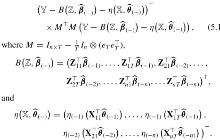
η(·) from typical realizations of the sample sizes ofn, T =10, 20, 30 are given inFigure 1.
Table 1indicates that the SMAVE method produces accurate estimates of bothβ0andθ0, and as eithernorTincreases, the MSEs of the estimates become smaller and smaller. Comparison of the results inTable 1with those in the second panel of table 1 by Xia and H¨ardle (2006) also suggests that the estimates and MSEs here are comparable with those in the article by Xia and H¨ardle (2006).
Example 5.2. Consider the following model:
Yit =(2Zit,1+Zit,2)/ √
5
+2 exp{−(2Xit+Xi,t−1+2Xi,t−2)2/3} +αi+vit,
(5.3)
Table 1. Means and MSEs of the estimates of the parameters in Example 5.1
10 20 30
n\T True value Mean MSE (×10−4) Mean MSE (
×10−4) Mean MSE (
×10−4)
10 β0=0.3000 0.2989 (4.3502) 0.3011 (2.1873) 0.3002 (1.4515)
θ0,1=0.5774 0.5789 (2.6539) 0.5783 (1.2542) 0.5769 (0.8428)
θ0,2=0.5774 0.5768 (2.6542) 0.5769 (1.2403) 0.5773 (0.8118)
θ0,3=0.5774 0.5763 (3.1450) 0.5768 (1.4429) 0.5778 (0.9853)
20 β0=0.3000 0.3012 (2.1887) 0.3006 (0.9868) 0.2998 (0.7108)
θ0,1=0.5774 0.5767 (1.3108) 0.5779 (0.6288) 0.5767 (0.4139)
θ0,2=0.5574 0.5786 (1.2686) 0.5766 (0.5951) 0.5771 (0.3705)
θ0,3=0.5774 0.5768 (1.4648) 0.5776 (0.6755) 0.5782 (0.4379)
30 β0=0.3000 0.2993 (1.5891) 0.2994 (0.6470) 0.3001 (0.4859)
θ0,1=0.5774 0.5770 (0.8558) 0.5767 (0.4155) 0.5769 (0.2822)
θ0,2=0.5774 0.5768 (0.8354) 0.5779 (0.3981) 0.5773 (0.2338)
θ0,3=0.5774 0.5783 (0.9518) 0.5775 (0.40812) 0.5778 (0.2374)
Figure 1. Curve estimates from single replications of the simulation study of Example 5.1. The solid curves are the true functionsη(X⊤ itθ0),
the dashed curves are the corresponding estimated functionsη(X⊤
itθ), and the dots denoteYit−Z⊤itβ−αiplotted againstX⊤itθ. The online version of this figure is in color.
whereZit =(Zit,1, Zit,2)⊤are two-dimensional iid (over both
i and t) random vectors with independent components that have binary distribution with P(Zit,j=0)=P(Zit,j=1)=
0.5, j =1,2, Xit=(Xit, Xi,t−1, Xi,t−2)⊤ in which Xit =
0.4Xi,t−1+xitandxit are iid (overiandt) and uniformly
dis-tributed withxit∼U(−1,1),vitare iid (overiandt) with
nor-mal distribution N(0,0.52), αi =0.5ZiA∗ +ui for i=1, . . . , n−1, and αn= −in=−11αi, in which ZiA∗ =
1 2T
T t=1(Zit,1 +Zit,2) and ui
iid
∼N(0,0.22). {Zit}, {xit}, {ui}, and {vit} are
mutually independent.
The true parameters of model (5.4) are β0=(2,1)⊤/ √
5 and θ0=(2,1,2)⊤/3, and the true link function is η(u)= 2 exp{−3u2}.
The means as well as the MSEs of the estimates of the param-eters over 200 replications are given inTable 2. These results indicate that the SMAVE method estimates the parameters accu-rately, and its performance (in terms of MSE) improves asnor
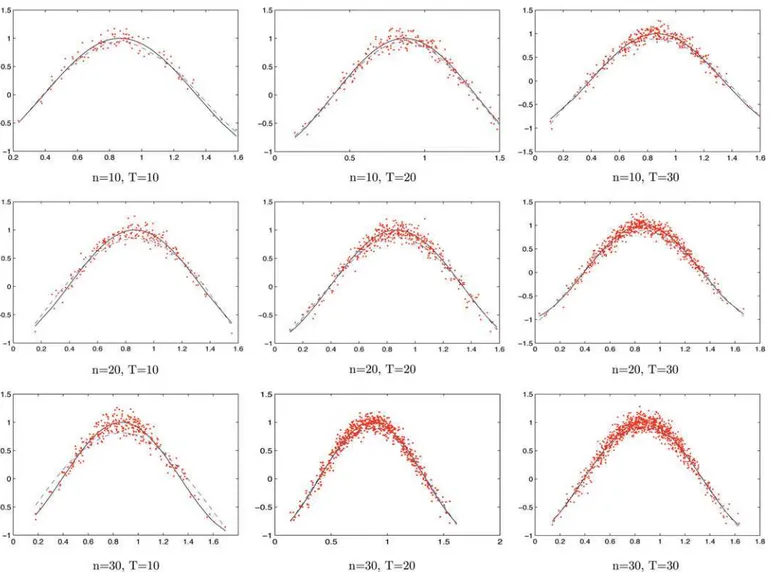
Tincreases. The estimates of the link functionη(·) from typical realizations of sample sizes ofn, T =10, 20, 30 are given in Figure 2.
5.2 Real Data Examples
5.2.1 U.S. Cigarette Demand. The first real data example is about the cigarette demand in 46 states of the United States over the period 1963–1992. The dataset is from the article by Baltagi, Griffin, and Xiong (2000), who used a linear dynamic panel data model of the form
lnCit =β0+β1lnCi,t−1+θ1lnDIit+θ2lnPit
+θ3lnPNit+uit (5.4)
to analyze the demand for cigarettes, where i=1, . . . , 46, denotes thei-th state,t =1, . . . ,29 denotes the t-th year,Cit
is the real per capita sales of cigarettes (measured in packs),
DIit is the real per capita disposable income,Pit is the average
retail price of a pack of cigarettes measured in real terms,PNit
is the minimum real price of cigarettes in any neighboring state, and the disturbance term uit in model (5.4) is specified
as
uit=μi+λt+vit, (5.5)
Table 2. Means and MSEs of the estimates of the parameters in Example 5.2
10 20 30
n\T True value Mean MSE (×10−4) Mean MSE (
×10−4) Mean MSE (
×10−4)
10 β0,1=0.8944 0.8901 (100.0000) 0.8787 (45.0000) 0.8875 (44.0000)
β0,2=0.4472 0.4422 (105.0000) 0.4538 (48.0000) 0.4484 (36.0000)
θ0,1=0.6667 0.6683 (13.0000) 0.6612 (5.7443) 0.6642 (4.7835)
θ0,2=0.3333 0.3281 (27.0000) 0.3400 (14.0000) 0.3320 (9.1121)
θ0,3=0.6667 0.6635 (15.0000) 0.6668 (7.6202) 0.6684 (4.3630)
20 β0,1=0.8944 0.9036 (57.0000) 0.8950 (26.0000) 0.8897 (18.0000)
β0,2=0.4472 0.4460 (52.0000) 0.4499 (33.0000) 0.4473 (19.0000)
θ0,1=0.6667 0.6651 (6.5923) 0.6639 (4.8670) 0.6662 (2.2190)
θ0,2=0.3333 0.3299 (16.0000) 0.3308 (9.4963) 0.3291 (4.4093)
θ0,3=0.6667 0.6679 (4.8119) 0.6693 (3.8523) 0.6686 (2.1373)
30 β0,1=0.8944 0.9012 (47.0000) 0.8940 (14.0000) 0.8932 (11.0000)
β0,2=0.4472 0.4505 (37.0000) 0.4484 (17.0000) 0.4495 (14.0000)
θ0,1=0.6667 0.6662 (4.9653) 0.6647 (2.3813) 0.6671 (1.0029)
θ0,2=0.3333 0.3299 (14.0000) 0.3323 (4.7590) 0.3316 (3.3297)
θ0,3=0.6667 0.6669 (5.2189) 0.6685 (0.40812) 0.6667 (1.0682)
Figure 2. Curve estimates from single replications of the simulation study of Example 5.2. The solid curves are the true functionsη(X⊤ itθ0),
the dashed curves are the corresponding estimated functionsη(X⊤
itθ), and the dots denoteYit−Z⊤itβ−αi plotted againstX⊤itθ. The online version of this figure is in color.
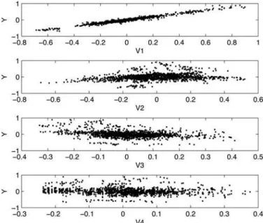
Figure 3. From top to bottom: the scatterplots ofYagainstV1,V2, V3, andV4.
where μi denotes a state-specific effect and λt denotes a
year-specific effect, which can also be interpreted as a trend in timet.
Due to the presence of the time-specific effect or trendλtin all
the variables, we first remove the trend from the log-transformed observations as in the article by Mammen, Støve, and Tjøstheim (2009),
Yit=lnCit−sC(t), V1it =Yi,t−1, V2it =lnDIit−sDI(t),
V3it =lnPit−sP(t), V4it =lnPNit−sPN(t),
where sC(t), sDI(t),sP(t), and sP N(t) are the nonparametric
estimates of the trends in lnCit, lnDIit, lnPit, and lnPNit
fori=1, . . . ,46 andt =1, . . . ,29. InFigure 3, we give the scatterplots ofY againstV1,V2,V3, andV4. It is clear from Figure 3thatYexhibits strong linearity withV1 (i.e., the lagged variable ofY). For the other three covariates, their linearities withY are not as strong as that for the lagged variable. Hence, we defineZit =V1it andXit =(V2it, V3it, V4it)⊤, and put Zit in the linear term andXit in the single-index term of the
following model:
Yit =Zitβ+g
X⊤itθ+αi+vit, (5.6)
whereθ=(θ1, θ2, θ3)⊤andαiis a state-specific effect that may
include religion, race, tourism, tax, and education. αi
corre-sponds to μi in models (5.4) and (5.5). Furthermore, as we
detrended lnCit, lnDIit, lnPit, and lnPNit, the year-specific
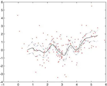
Figure 4. Estimated link function and its 95% confidence band for the cigarette demand data. Dots denote Yit−Zitβ−αi plotted againstX⊤
itθ. The solid line denotes the estimated link functionη(X⊤itθ). The dash-dotted lines represent the 95% confidence band. The online version of this figure is in color.
term λt that appeared in model (5.4) and (5.5) is eliminated
from model (5.6).
After applying the estimation method proposed in Section 2 to the data on Yit,Zit,Xit, we obtain the estimates of the
parameters in model (5.6), which are summarized inTable 3. The estimated curve of the link function as well as its 95% confidence band is given inFigure 4.
A comparison of the results inTable 3with that in the article by Baltagi, Griffin, and Xiong (2000) indicates that our estimate ofβis smaller than the estimate of the corresponding coefficient by Baltagi, Griffin, and Xiong (2000), where a value of 0.90 from the OLS and a value of 0.91 from the GLS were obtained. In addition, compared with θ=(0.2112,−0.9404,0.2665)⊤
from the OLS and θ =(0.1602,−0.9503,0.2669)⊤ from the
GLS in the article by Baltagi, Griffin, and Xiong (2000), the absolute value of our estimate ofθ2 is smaller, while those of
θ1andθ3are larger (note that due to the identification condition θ =1, one has to normalize the estimates ofθin model (5.4) before making comparisons). The computed coefficient of de-termination for model (5.6) isR2=0.9698, which indicates a good fit to the data.
5.2.2 Foreign Direct Investment and Economic Growth. There has been a vast literature on the effect of FDI on the economic growth of the hosting country. Some recent research (Kottaridi and Stengos 2010) found that the relationship be-tween FDI and economic growth is nonlinear. In this article, we focus our study on 22 OECD countries over the period 1970– 2000. According to data availability, the following countries are
Table 3. Estimates of the parameters in the cigarette data example
β θ1 θ2 θ3
Detr. log-sales in Detr. log-disposable Detr. log-price Detr. log-min price Parameter previous year per capita income per pack in neighboring states
Estimate 0.8480 0.2594 –0.8735 0.4119
(SD) (0.0073) (0.0217) (0.0099) (0.0260)
Table 4. Estimates of the parameters in the FDI data example
β1 β2 θ1 θ2 θ3
Parameter Log-GFCF Log-initial GDP Log-FDI Years schooling Population growth
Estimate 4.6605 −1.2880 0.6905 0.3409 0.6380
(SD) (0.5235) (0.1319) (0.0280) (0.0195) (0.0403)
selected: Australia, Austria, Belgium, Canada, Denmark, Fin-land, France, Germany, Greece, IceFin-land, IreFin-land, Japan, Repub-lic of Korea, Mexico, Netherlands, Norway, Portugal, Spain, Sweden, Turkey, the United Kingdom, and the United States. As is conventional in the literature, we use 5-year averages to reduce the impact of year-to-year fluctuations in output. We use the partially linear single-index structure to model the effects of FDI, human capital (measured by average years of schooling), population growth, as well as domestic investment (measured by gross fixed capital formation, GFCF) on growth. This relaxes the restrictions on the form of effects while at the same time retaining much of the ease of interpretation of linear models. More specifically, we use the following model specification:
Yit =Z⊤itβ0+η
X⊤ itθ0
+αi+vit, 1≤i≤21, 1≤t ≤7,
(5.7)
where idenotes countryi,t denotes thetth 5-year period,Yit
denotes GDP per capita growth,Zit=(Zit,1, Zit,2)⊤withZit,1 denoting log of GFCF in percentages of GDP andZit,2 denot-ing log of GDP per capita at the beginndenot-ing of thet-th 5-year period,Xit=(Xit,1, Xit,2, Xit,3)⊤ withXit,1 representing log-FDI in percentages of GDP,Xit,2representing average years of schooling, andXit,3representing population growth.
The data on FDI are obtained from the United Nations Con-ference on Trade and Development (UNCTAD). Data on the other variables are obtained from the World Development Indi-cators (WDI) of the World Bank, and GDP per capita, FDI, and gross fixed formation are all measured in constant 2000 U.S.
Figure 5. Estimated link function and its 95% confidence band for the FDI data. The solid line denotes the estimated link functionη(X⊤
itθ). The dash-dotted lines represent the 95% confidence band. The online version of this figure is in color.
dollars. Kottaridi and Stengos (2010) employed a partially linear model to the same data where a general nonparametric termg(Xit) is used in place ofη(X⊤itθ0). They found that FDI inflows and human capital have nonlinear effects on growth in the OECD countries. AsXit is three-dimensional, the use of
the single-index termη(X⊤
itθ0) here avoids the “curse of dimen-sionality” that would arise due to the sparsity of data available for the estimation ofg(·) ifg(Xit) were used. Hence, the use of
model (5.7) leads to more reliable estimates of the effects of the factors on economic growth. The estimated parameters and their standard deviations are given inTable 4, and the estimated link function together with its 95% confidence band is shown in Fig-ure 5. The confidence band is obtained by the plug-in method. We have also used the wild bootstrap method to calculate the confidence band, and the result is similar.
The results indicate that GDP growth has a positive relation-ship with domestic investment whereas it is negatively related to the initial per capita income. Moreover, FDI, human capital, and population growth have overall positive relationships with GDP growth except that when the linear combination of these three variables is between 2.3 and 3.2, the relationships are reversed (as can be seen from the trough at around 3.2 in the plot of the estimated link function).
6. CONCLUSIONS AND DISCUSSION
This article has considered a partially linear single-index panel data model with fixed effects. A SMAVE method associ-ated with a dummy variable approach has been proposed to deal with the estimation of both the parametric and nonparametric components of the model. We have shown that the proposed es-timators are all asymptotically normally distributed regardless of whether the effects involved are random or fixed. We have then assessed the finite sample performance of the proposed estimation method through using both simulated and real data examples.
In this article, we focus on the case where bothnandT are very large and establish the asymptotic theory for the case of
n, T → ∞simultaneously. It is quite straightforward to extend our methodology and theory to the case wheren is small but
T is large, the analysis under which it is similar to the time series case. It is also possible to extend our methodology to the case wheren is large but T is small. However, for this latter case, the asymptotic theory would be more complicated for the fixed effects model, and the asymptotic variance would rely on
T. In terms of asymptotic theory, another important question is whether our estimators in Section 2 could achieve a semi-parametric efficiency bound in the panel data setting, as most of the existing semiparametric efficiency results are established under the cross-section framework (see, e.g., Bickel et al.1993; Carroll et al. 1997). We will address this semiparametric
efficiency issue in our future research as different techniques would be involved.
Another interesting topic is to allow the existence of individ-ual effects for the parameters in both the linear and single-index components of our model. For example, we can consider
β=β0+βi, θ=θ0+θi,
where (β⊤i ,θ⊤i )⊤, 1≤i≤n, are iid and follow a multivariate
normal distribution with zero mean. Under such assumptions, our model is quite similar to the semiparametric mixed effects models discussed by Wu and Zhang (2006). However, to con-struct consistent estimators ofβ0,θ0,andη(·), the estimation methodology in Section2would need to be modified substan-tially. Hence, we will consider this issue in our future study.
APPENDIX A: ASSUMPTIONS
Let Zi=(Zit : 1≤t ≤T), Xi=(Xit : 1≤t≤T), and Vi =(vit: 1≤t≤T). To derive the consistency of the initial
estimatesβandθ, we need the following set of regularity con-ditions.
A1 (Zi,Xi, Vi),i=1, . . . , n, are iid and{(Zit,Xit, vit) :t ≥
1}is a stationary α-mixing sequence with mixing coeffi-cientαi(t) for eachi. Furthermore, there exists a positive
coefficient functionα(t) such that
sup
i
αi(t)≤α(t) with α(t)≤Cαt−γ0,
where Cα>0 and γ0> (2+2(δδ∗−)(2δ+δ)
∗) , in which δ is chosen such thatEXit2+δ <∞andδ∗< δ is chosen such that
E[|vit|2+δ∗]<∞, · is theL2-distance. A2 The kernel function H(·): Rp
→R+ is a bounded and
Lipschitz continuous probability density function with a compact support. Furthermore, H(x) is symmetric and
xx⊤H(x)dxis positive definite.
A3 The density functionfX(·) ofXitis second-order continuous
and has gradientfX′(·). Moreover,fX(·) is positive over its compact supportX∗.
A4 Letg1(x) :=E[Zit|Xit =x] and g2(x) :=E[ZitZ⊤it|Xit =
x]. Both g1(x) and g2(x) have bounded and continuous derivatives. In addition,EZit2+δ<∞and
E{(Zit−E(Zit|Xit)) (Zit−E(Zit|Xit))⊤}
is a positive definite matrix, whereδis the same as defined inA1.
A5 Additionally, suppose that {vit} is independent of
{(Zit,Xit)}withE[vit]=0 and 0< σ2:=E[vit2]<∞.
A6 The link functionη(·) has continuous derivatives of up to the second order.
A7 The bandwidth h1 involved in the multivariate weights satisfies
h1→0, logT
T hp1+2 =O(1),
(nT)2γ0−4p−3h2pγ0+4p 2+9p+2 1
log2γ0−4p+1(nT) → ∞,
wherepis the dimension ofXit, andγ0andδare the same as defined inA1.
To establish asymptotic distribution for the final parametric estimatorsβandθ, we further need the following set of regu-larity conditions.
B1 The kernel functionK(·):R→R+is a bounded and
sym-metric probability density function with a compact support. Furthermore, K(·) is differentiable and has a continuous derivative.
B2 The density functionfθ(·) ofX⊤itθ is positive and
second-order continuous with respect toθin a neighborhood ofθ0. Moreover,fθ0(·) is positive over its compact supportX∗(θ). B3 The conditional expectationg3(u) :=E[Zit|X⊤itθ=u] has
a bounded and continuous derivative with respect toθ in a neighborhood ofθ0.
B4 The bandwidth h2 involved in the single-index weights satisfies
0< lim
n,T→∞(nT)h 5 2<∞.
Furthermore, there exists a relationship betweennandT,
Tδ∗δ+2δ+32p+16δplog5(2+δ)(2+δ∗−2p)(nT)
n4δδ∗+10δ∗−2δ−32p−16δp =o(1).
In A1, we assume that (Zi,Xi, Vi), 1≤i≤n are
cross-sectional independent (see, e.g., Su and Ullah 2006; Sun, Carroll, and Li2009) and each time series isα-mixing depen-dent, which can be satisfied by many linear and nonlinear time series (see such models discussed in Section 4). Assumption A2 involves some mild conditions on the multivariate kernel functionH(·).A3andA4are similar to the corresponding con-ditions by Xia and H¨ardle (2006). Sinceαi are allowed to be
correlated with (Xit,Zit),uit=αi+vitthus may be correlated
with (Xit,Zit) even though vit are independent of (Xit,Zit).
AssumptionA4is needed to ensure that both (β0,θ0) andη(·) are identifiable and estimable. Meanwhile, the independence between{(Zit,Xit)}and{vit}inA5is imposed to simplify our
proofs and it can be removed at the expense of more tedious proofs. A6is a common condition for local linear estimation (see, e.g., Fan and Gijbels1996; Fan and Yao2003). We next show that the bandwidth restrictions in A7are satisfied under mild conditions if we takeh1∼(nT)−ϑ, 0< ϑ <1/(p+2). It is easy to check thath1∼(nT)−ϑ =o(1) and the second condi-tion inA7is also satisfied whenn=O(Tϑ(p1+2)−1/log
1
ϑ(p+2)T). If we letp1=2γ0−4p−3,p2=2pγ0+4p2+9p+2,and
p3 =2γ0−4p+1, the left-hand side of the last term in A7 becomes
(nT)p1hp2 1 logp3(nT) =
(nT)p1−p2ϑ logp3(nT),
which tends to ∞ when p1 > p2ϑ. As ϑ <1/(p+2), 2− 2pϑ >0. By some elementary calculation, it is easy to show that if
γ0 >
(4p2+9p+2)ϑ
2−2pϑ +
4p+3 2−2pϑ,
thenp1> p2ϑand thus the third condition inA7holds. AssumptionsB1–B3are natural extensions of conditions C2, C4, and C5 in the article by Xia and H¨ardle (2006). The rate of the bandwidth h2 inB4 is optimal for pooled local linear estimators. In particular, ifδ > δ∗≫p, we can show that the
second condition inB4 could include two cases: (i) the time series length T is larger than the cross-sectional dimensionn, and (ii) the cross-sectional dimensionnis larger than the time series lengthT.
APPENDIX B: PROOF OF THEOREM 3.1
Define ax=η(x⊤θ0), ait =η(X⊤itθ0), bx=η′(x⊤θ0), and
bit=η′(X⊤itθ0). Letax,ait,bx, andbitbe the local linear
estima-tors obtained from Equation (2.6) using the set of multivariate weights in Equation (2.8). Letex,∗,Xx,∗,Xx,∗,Wx,andZx,∗be
the counterparts ofeit,∗,Xit,∗,Xit,∗,Wit, andZit,∗whenXit is
replaced byx. Furthermore, define
Dx,∗=D−D(D⊤WxD)−1D⊤WxD, we need to establish asymptotic uniform expansions foraxand
bxforx∈X∗.
Lemma B.1. Let AssumptionsA1–A7in Appendix A hold. Then, we have
D.4 in the online supplementary material, we have uniformly
forx∈X∗,
By Lemmas D.4 and D.5 in Appendix D of the online sup-plementary material, we also have
(1,0)X⊤x,∗(θ)WxXx,∗(θ)
On the other hand, by Lemma D.4, we have, uniformly for x∈X∗,
We next give the proof of Theorem 3.1 by making use of Lemma B.1.
Proof of Theorem 3.1. By Equations (2.7) and (B.1), and following the same arguments as used in the proof of Lemma 1 by Xia and H¨ardle (2006), we have
Since we use the multivariate kernelH(·) for producing initial estimates ofβ0andθ0, Equation (B.11) does not involveθ. From process of producing initial estimates.
By Assumption A4 in Appendix A, it can be shown that the matrixE[ZitZ⊤it]−E[g1(Xit)g1⊤(Xit)] is positive
def-inite. Similarly to the proofs of lemma 1 and theorem 1 by Xia and H¨ardle (2006), the eigenvalues of the matrix (E[ZitZ⊤it])−
1E[g
1(Xit)g⊤1(Xit)] are all less than 1. Hence, after
a sufficiently large number of iterations, we have
βk−β0=oP(1),
which implies that the first result in Equation (3.1) holds. By Equations (2.7) and (B.2), we have
θ−θ0=(θ⊤θ0)−1(1−θ⊤θ0)θ0+O(ζβ)+oP(1),
(B.13) which implies
θ=(θ⊤θ0)−1θ0+O(ζβ)+oP(1). (B.14)
Following the proof of lemma 1 by Xia and H¨ardle (2006), we can also show that the second result in Equation (3.1) holds.
APPENDIX C: PROOFS OF THEOREMS 3.2 AND 3.3
For simplicity, letWit(θ) be defined asWitwith the weights in Equation (2.7) replaced by those in Equation (2.8), andeit,∗,
Xit,∗, Xit,∗,Vit, andZit,∗ be defined in the same way as in Appendix B. Throughout this section, ax,ait, bx, and bit are
the local linear estimators obtained from Equation (2.6) using the single-index weights defined in Equation (2.9). As in Ap-pendix B, ex,∗, Xx,∗, Xx,∗, Wx(θ),Vx,∗, and Zx,∗ are defined
similarly toeit,∗,Xit,∗,Xit,∗,Wit(θ),Vit,∗, and Zit,∗ withXit
replaced byx. Furthermore, define
dx(θ)= d11⊤(x)θ
To prove the asymptotic distributions ofβandθgiven in The-orem 3.2, we need the following asymptotic uniform expansions ofaxandbxforx∈X∗.
By Equation (C.3), Lemma D.3 in the online supplementary material, and the same Taylor expansion forη(X⊤
itθ0) as in the proof of Lemma B.1, we complete the proofs of Equations (C.1)
and (C.2).
Before giving the proof of Theorem 3.2, we introduce the following notations. Let
Proof of Theorem 3.2. Since the main idea of the proof is a nontrivial extension of the proof of theorem 1 by Xia and H¨ardle (2006), we still need to provide the following details.
By Lemma C.1 and following the proof of lemma 6.3 by Xia and H¨ardle (2006), we have
Following the proof of Lemma D.4 in Appendix D of the online supplementary material, we have
JnT −→P
Similarly to the proof of theorem 1 by Xia and H¨ardle (2006), it can be shown that a matrix of the formN:=(J−1)1/2U(J−1)1/2 is a semipositive definite matrix with rank d+p−1 and all eigenvalues being less than 1. Let 1> λ1≥λ2 ≥ · · · ≥
λd+p−1 >0 be the eigenvalues ofN.
LetJnT(k) andUnT(k) be the corresponding versions ofJnT and UnT at the k-th iteration. Then, by Equations (C.5) and (C.6), the eigenvalues of
which, together with the proof of Lemma D.5, implies
ζrk+1 ≤τnT(2)+λ1(k)ζrk +c0ζrk By Theorem 3.1, we have
ζr1 ≤
for allk≥1. Then, following the proof of theorem 1 by Xia and H¨ardle (2006), we have, for sufficiently largek,
ζrk+1 =OP By some standard arguments, it can be shown that the leading term ofMnT is
asnT → ∞. Applying a standard central limit theorem forα -mixing processes (see, e.g., theorem 2.21 by Fan and Yao2003), we have
√
nTM∗nT −→d N(0,1). (C.15) By Equations (C.4) and (C.13)–(C.15), we have shown that
Theorem 3.2 holds.
Proof of Theorem 3.3. By the definition of local linear esti-mators, it is easy to show that
η(x⊤θ)−η(x⊤θ0) By Theorem 3.2, we have
nT(3)=OP((nT)−1/2). (C.16)
Meanwhile, by the property of local linear smoothing, we have
We next turn to the asymptotic distribution ofnT(2). ByB1,
By Theorem 3.2 and following the same argument as in the proof of Lemma D.5 of the online supplementary material, we have
nT(2,2)=oP(1), (C.18)
which implies that the leading term of √1 nT h2
In a similar way to the proof of theorem 2.21 by Fan and Yao (2003), applying Doob’s large-block and small-block argument in the proof of asymptotic normality for the nonparametric ker-nel estimator under α-mixing dependence, we can show that
nT(2,1) (C.19), and the uniform convergence results in Appendix D of the online supplementary material, we have
nT(2)
The supplementary materials give some uniform consistency results for nonparametric kernel estimators, which have been used to prove the asymptotic results in Appendices B and C.
ACKNOWLEDGMENTS
We are grateful to the editor, associate editor, and two ref-erees for their helpful comments, which greatly improved the
former version of the article. We also thank Xiaohong Chen, Qi Li, Oliver Linton, Liangjun Su, and the seminar partici-pants at Monash University, University of Adelaide, University of Queensland, SETA 2011 Conference in Melbourne, ESAM 2011 Conference in Adelaide, and the 8th World Congress in Probability and Statistics in Istanbul. This project is financially supported by the Australian Research Council Discovery Grants Program under Grant Number: DP0879088. The first author’s research is supported by the Start-Up Fund from University of Queensland and the third author’s research is supported by the Australian Research Council Discovery Early Career Re-searcher Award under Grant Number: DE120101130 and the Monash Researcher Accelerator Plan. The corresponding au-thor of this article is Dr Degui Li.
[Received August 2011. Revised December 2012.]
REFERENCES
An, H. Z., and Huang, F. C. (1996), “The Geometrical Ergodicity of Nonlinear Autoregressive Models,”Statistica Sinica, 6, 943–956. [319]
Arellano, M. (2003),Panel Data Econometrics, Oxford: Oxford University Press. [315]
Bai, Y., Fung, W., and Zhu, Z. (2009), “Penalized Quadratic Inference Functions for Single-Index Models With Longitudinal Data,”Journal of Multivariate Analysis, 100, 152–161. [316]
Baltagi, B. H. (1995),Econometric Analysis of Panel Data, New York: John Wiley. [315]
Baltagi, B. H., Griffin, J. M., and Xiong, W. (2000), “To Pool or Not to Pool: Ho-mogenous Versus Heterogenous Estimators Applied to Cigarette Demand,”
Review of Economics and Statistics, 82, 117–126. [316,321,323] Bickel, P. J., Klaassen, C. A. J., Ritov, Y., and Wellner, J. A. (1993),Efficient
and Adaptive Estimation for Semiparametric Models, Baltimore, MD: The Johns Hopkins University Press. [324]
Cai, Z., and Li, Q. (2008), “Nonparametric Estimation of Varying Coef-ficient Dynamic Panel Data Models,” Econometric Theory, 24, 1321– 1342. [315,319]
Carroll, R. J., Fan, J., Gijbels, I., and Wand, M. (1997), “Generalized Partially Linear Single-Index Models,”Journal of the American Statistical Associa-tion, 92, 477–489. [316,318,320,324]
Chen, J., Gao, J., and Li, D. (2013), “Estimation in Single-Index Panel Data Models With Heterogeneous Link Functions,”Econometric Reviews, 32, 928–955. [316]
Chen, J., Gao, J., and Li, D. (2012), “Semiparametric Trending Regression in Panel Data Models With Cross-Sectional Dependence,”Journal of Econo-metrics, 171, 71–85. [315]
Fan, J., and Gijbels, I. (1996),Local Polynomial Modeling and Its Applications, London: Chapman & Hall. [325]
Fan, J., and Yao, Q. (2003),Nonlinear Time Series: Nonparametric and Para-metric Methods, New York: Springer. [315,325,328,329]
Gao, J. (2007),Nonlinear Time Series: Semiparametric and Nonparametric Methods, London: Chapman & Hall/CRC. [315]
Henderson, D., Carroll, R., and Li, Q. (2008), “Nonparametric Estimation and Testing of Fixed Effects Panel Data Models,”Journal of Econometrics, 144, 257–275. [315,316]
Henderson, D., and Ullah, A. (2005), “A Nonparametric Random Effects Esti-mator,”Economics Letters, 88, 403–407. [316]
Hjellvik, V., Chen, R., and Tjøstheim, D. (2004), “Nonparametric Estimation and Testing in Panels of Intercorrelated Time Series,”Journal of Time Series Analysis, 25, 831–872. [315]
Hsiao, C. (2003),Analysis of Panel Data, Cambridge: Cambridge University Press. [315,316]
Kottaridi, C., and Stengos, T. (2010), “Foreign Direct Investment, Human Capi-tal and Non-Linearities in Economic Growth,”Journal of Macroeconomics, 32, 858–871. [323,324]
Li, D., Chen, J., and Gao, J. (2011), “Non-Parametric Time-Varying Coefficient Panel Data Models With Fixed Effects,”Econometrics Journal, 14, 387–408. [316]
Li, Q., and Racine, J. (2007), Nonparametric Econometrics, Princeton, NJ: Princeton University Press. [315]
Li, Q., and Stengos, T. (1996), “Semiparametric Estimation of Partially Linear Regression Models,”Journal of Econometrics, 71, 389–397. [316] Liang, H., Liu, X., Li, R., and Tsai, C. (2010), “Estimation and Testing for
Partially Linear Single-Index Models,”The Annals of Statistics, 38, 3811– 3836. [316,318,320]
Mammen, E., Støve, B., and Tjøstheim, D. (2009), “Nonparametric Additive Models for Panels of Time Series,” Econometric Theory, 25, 442–481. [315,316,323]
Phillips, P. C. B., and Moon, H. (1999), “Linear Regression Limit Theory for Nonstationary Panel Data,”Econometrica, 67, 1057–1111. [317,318] Powell, J. J., Stock, J. H., and Stoker, T. M. (1989), “Semiparametric Estimation
of Index Coefficients,”Econometrica, 57, 1403–1430. [319]
Su, L., and Ullah, A. (2006), “Profile Likelihood Estimation of Partially Linear Panel Data Models With Fixed Effects,”Economics Letters, 92, 75–81. [316,325]
Sun, Y., Carroll, R. J., and Li, D. (2009), “Semiparametric Estimation of Fixed Effects Panel Data Varying Coefficient Models,”Advances in Econometrics, 25, 101–129. [316,320,325]
Ullah, A., and Roy, N. (1998), “Nonparametric and Semiparametric Economet-rics of Panel Data,” inHandbook of Applied Economics Statistics, eds.
A. Ullah and D.E.A. Giles, New York: Marcel Dekker, pp. 579–604. [315,316]
Wang, J., Xue, L., Zhu, L., and Chong, Y. (2010), “Estimation for a Partially– Linear Single-Index Model,”The Annals of Statistics, 38, 246–274. [316] Wu, H., and Zhang, J. (2006),Nonparametric Regression Methods for
Longi-tudinal Data Analysis: Mixed-Effects Modeling Approaches, Hoboken, NJ: Wiley. [320,325]
Xia, Y. (2006), “Asymptotic Distributions for Two Estimators of the Single-Index Model,”Econometric Theory, 22, 1112–1137. [317]
Xia, Y., and H¨ardle, W. (2006), “Semi-Parametric Estimation of Partially Linear Single-Index Models,”Journal of Multivariate Analysis, 97, 1162–1184. [316,317,318,320,325,326,327,328]
Xia, Y., Tong, H., and Li, W. K. (1999), “On Extended Partially Linear Single-Index Models,”Biometrika, 86, 831–842. [319]
Xia, Y., Tong, H., Li, W. K., and Zhu, L. (2002), “An Adaptive Estimation of Dimension Reduction Space,”Journal of the Royal Statistical Society,
Series B, 64, 363–410. [316,317,318]
Yu, Y., and Ruppert, D. (2002), “Penalized Spline Estimation for Partially Linear Single-Index Models,”Journal of the American Statistical Association, 97, 1042–1054. [316]