Full Terms & Conditions of access and use can be found at
http://www.tandfonline.com/action/journalInformation?journalCode=ubes20
Download by: [Universitas Maritim Raja Ali Haji] Date: 12 January 2016, At: 17:19
Journal of Business & Economic Statistics
ISSN: 0735-0015 (Print) 1537-2707 (Online) Journal homepage: http://www.tandfonline.com/loi/ubes20
Inhomogeneous Dependence Modeling with
Time-Varying Copulae
Enzo Giacomini, Wolfgang Härdle & Vladimir Spokoiny
To cite this article: Enzo Giacomini, Wolfgang Härdle & Vladimir Spokoiny (2009)
Inhomogeneous Dependence Modeling with Time-Varying Copulae, Journal of Business & Economic Statistics, 27:2, 224-234, DOI: 10.1198/jbes.2009.0016
To link to this article: http://dx.doi.org/10.1198/jbes.2009.0016
Published online: 01 Jan 2012.
Submit your article to this journal
Article views: 227
View related articles
Inhomogeneous Dependence Modeling with
Time-Varying Copulae
Enzo G
IACOMINIHumboldt-Universita¨t zu Berlin, Center for Applied Statistics and Economics, 10099 Berlin, Germany; and
Weierstrass Institute for Applied Analysis and Stochastics, 10117 Berlin, Germany (giacomini@wiwi.hu-berlin.de)
Wolfgang H
A¨ RDLEHumboldt-Universita¨t zu Berlin, Center for Applied Statistics and Economics, 10099 Berlin, Germany
(haerdle@wiwi.hu-berlin.de)
Vladimir S
POKOINYWeierstrass Institute for Applied Analysis and Stochastics, 10117 Berlin, Germany; and Humboldt-Universita¨t zu
Berlin, Department of Mathematics, 10099 Berlin, Germany (spokoiny@wias-berlin.de)
Measuring dependence in multivariate time series is tantamount to modeling its dynamic structure in space and time. In risk management, the nonnormal behavior of most financial time series calls for non-Gaussian dependences. The correct modeling of non-non-Gaussian dependences is, therefore, a key issue in the analysis of multivariate time series. In this article we use copula functions with adaptively estimated time-varying parameters for modeling the distribution of returns. Furthermore, we apply copulae to the estimation of Value-at-Risk of portfolios and show their better performance over theRiskMetricsapproach.
KEY WORDS: Adaptive estimation; Nonparametric estimation; Value-at-Risk.
1. INTRODUCTION
Time series of financial data are high dimensional and typ-ically have a non-Gaussian behavior. The standard modeling approach based on properties of the multivariate normal dis-tribution therefore often fails to reproduce the stylized facts (i.e., fat tails, asymmetry) observed in returns from financial assets.
A correct understanding of the time-varying multivariate (conditional) distribution of returns is vital to many standard applications in finance such as portfolio selection, asset pric-ing, and Value-at-Risk (VaR) calculation. Empirical evidence from asymmetric return distributions have been reported in the recent literature. Longin and Solnik (2001) investigate the distribution of joint extremes from international equity returns and reject multivariate normality in their lower orthant; Ang and Chen (2002) test for conditional correlation asymmetries in U.S. equity data, rejecting multivariate normality at daily, weekly, and monthly frequencies; and Hu (2006) models the distribution of index returns with mixtures of copulae, finding asymmetries in the dependence structure across markets. For a concise survey on stylized empirical facts from financial returns see Cont (2001) and Granger (2003).
Modeling distributions with copulae has drawn attention from many researchers because it avoids the ‘‘procrustean bed’’ of normality assumptions, producing better fits of the empirical characteristics of financial returns. A natural extension is to apply copulae in a dynamic framework with conditional dis-tributions modeled by copulae with time-varying parameters. The question, though, is how to steer the time-varying copulae parameters. This question is the focus of this article.
A possible approach is to estimate the parameter from structurally invariant periods. There is a broad field of econo-metric literature on structural breaks. Tests for unit root in macroeconomic series against stationarity with a structural
break at a known change point have been investigated by Perron (1989), and for an unknown change point by Zivot and Andrews (1992), Stock (1994) and Hansen (2001); Andrews (1993) tests for parameter instability in nonlinear models; Andrews and Ploberger (1994) construct asymptotic optimal tests for multiple structural breaks. In a different set up, Quintos, Fan, and Philips (2001) test for a constant tail index coefficient in Asian equity data against a break at an unknown point.
Time-varying copulae and structural breaks are combined in Patton (2006). The dependence structure across exchange rates is modeled with time-varying copulae with a parameter specified to evolve as an Autoregressive Moving Average (ARMA)-type process. Tests for a structural break in the ARMA coefficients at a known change point have been performed, and strong evidence of a break was found. In a similar fashion, Rodriguez (2007) models the dependence across sets of Asian and Latin American stock indexes using time-varying copula where the parameter follows regime-switching dynamics. Common to these articles is that they use a fixed (parametric) structure for the pattern of changes in the copula parameter.
In this article we follow a semiparametric approach, because we are not specifying the parameter changing scheme. Rather, we select locally the time-varying copula parameter. The choice is performed via an adaptive estimation under the assumption of local homogeneity: For every time point there exists an interval of time homogeneity in which the copula parameter can be well approximated by a constant. This interval is recovered from the data using local change point analysis. This does not imply that the model follows a change point structure. The adaptive
esti-224
2009 American Statistical Association Journal of Business & Economic Statistics April 2009, Vol. 27, No. 2 DOI 10.1198/jbes.2009.0016
mation also applies when the parameter varies smoothly from one value to another (see Spokoiny 2009).
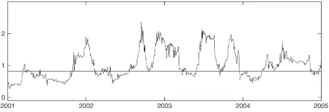
Figure 1 shows the time-varying copula parameter determined by our procedure for a portfolio composed of daily prices of six German equities and the ‘‘global’’ copula parameter, shown by a constant horizontal line. The absence of parametric specifi-cation for time variations in the dependence structure (its dynamics is obtained adaptively from the data) allows for flexibility in estimating dependence shifts across time.
The obtained time-varying dependence structure can be used in financial engineering applications, the most prominent being the calculation of the VaR of a portfolio. Using copulae with adaptively estimated dependence parameters we estimate the VaR from Deutscher Aktienindex (DAX) portfolios over time.
As a benchmark procedure we choose RiskMetrics, a widely
used methodology based on conditional normal distributions
with a Generalized Autoregressive Conditional
Hetero-scedasticity (GARCH) specification for the covariance matrix. Backtesting underlines the improved performance of the pro-posed adaptive time-varying copulae fitting.
This article is organized as follows: Section 2 presents the basic copulae definitions, Section 3 discusses the VaR and its estimation procedure. The adaptive copula estimation is ex-posed in Section 4 and is applied to simulated data in Section 5. In Section 6, the VaR from DAX portfolios is estimated based on adaptive time-varying copulae. The estimation performance
is compared with the RiskMetrics approach by means of
backtesting. Section 7 concludes.
2. COPULAE
Copulae merge marginal distributions into joint distributions, providing a natural way for measuring the dependence structure between random variables. Copulae are present in the literature since Sklar (1959), although related concepts originate in Hoeffding (1940) and Fre´chet (1951), and have been widely studied in the statistical literature (see Joe 1997, Nelsen 1998, and Mari and Kotz 2001). Applications of copulae in finance, insur-ance, and econometrics have been investigated in Embrechts, McNeil, and Straumann (2002); Embrechts, Hoeing, and Juri (2003a); Franke, Ha¨rdle, and Hafner (2004); and Patton (2004) among others. Cherubini, Luciano, and Vecchiato (2004) and McNeil, Frey, and Embrechts (2005) provide an overview of copulae for practical problems in finance and insurance.
Assuming absolutely continuous distributions and con-tinuous marginals throughout this article, we have from Sklar’s
theorem that for ad-dimensional distribution functionFwith marginal cdf’sF1,. . .,Fdthere exists a unique copulaC: [0,
where F(s), s 2 R stands for the one-dimensional standard normal cdf,FYis the cdf ofY¼(Y1,. . .,Yd)>;Nd(0,C),0is the (d31) vector of zeros, andCis a correlation matrix. The Gaussian copula represents the dependence structure of the multivariate normal distribution. In contrast, the Clayton cop-ula given by
foru> 0, expresses asymmetric dependence structures. The dependence at upper and lower orthants of a copulaC may be expressed by the upper and lower tail dependence coefficients lU ¼ limu!0Cbðu;. . .;uÞ=u and lL ¼ limu!0
Cðu;. . .;uÞ=u, whereu2(0, 1] andCbis the survival copula of C(see Joe 1997 and Embrechts, Lindskog, and McNeil 2003b). Although Gaussian copulae are asymptotically independent at the tails (lL ¼lU ¼0), the d-dimensional Clayton copulae exhibit lower tail dependence (lL¼d1/
u
) but are asymptoti-cally independent at the upper tail (lU¼0). Joe (1997) pro-vides a summary of diverse copula families and detailed description of their properties.
For estimating the copula parameter, consider a sample fxtgT
t¼1of realizations fromXwhere the copula ofXbelongs to
a parametric family C ¼ fCu;u2Qg: Using Equation (2.1), andfjis the probability density function of Fj. The canonical maximum likelihood estimator ^u maximizes the pseudo log-likelihood with empirical marginal cdf’s L~ðuÞ ¼PTt¼1logc
fFb1ðxt;1Þ;. . .;Fbdðxt;dÞ;ugwhere
Figure 1. Time-varying dependence. Time-varying dependence parameter and global parameter (horizontal line) estimated with Clayton copula, stock returns from Allianz, Mu¨nchener Ru¨ckversicherung, BASF, Bayer, DaimlerChrysler, and Volkswagen.
b
cummulative distribution function by the denominatorTþ1. This ensures thatfFb1ðxt;1Þ;. . .;Fbdðxt;dÞg>2 ð0;1Þdand avoids
infinite values the copula density may take on the boundary of the unit cube (see McNeil, Frey, and Embrechts 2005). Joe (1997); Cherubini, Luciano, and Vecchiato (2004); and Chen and Fan (2006) provide a detailed exposition of inference methods for copulae.
3. VALUE-AT-RISK AND COPULAE
The dependence (over time) between asset returns is espe-cially important in risk management, because the profit and loss (P&L) function determines the VaR. More precisely, the VaR of a portfolio is determined by the multivariate dis-tribution of risk factor increments. Ifw¼ ðw1;. . .;wdÞ>2Rd
denotes a portfolio of positions on d assets and St¼
ðSt;1;. . .;St;dÞ>a nonnegative random vector representing the
prices of the assets at timet, the valueVtof the portfoliowis
given byVt ¼P
d
j¼1wjSt;j. The random variable
Lt¼ðVtVt1Þ; ð3:1Þ
called the profit and loss (P&L) function, expresses the change in the portfolio value between two subsequent time points. Defining the log-returns Xt¼ ðXt;1;. . .;Xt;dÞ>; where Xt,j ¼
It follows from Equation (3.2) thatFt;Lt depends on the
spec-ification of thed-dimensional distribution of the risk factorsXt.
Thus, modeling their distribution over time is essential for obtaining the quantiles (Eq. 3.3).
TheRiskMetricstechnique, a widely used methodology for VaR estimation, assumes that risk factors Xt follow a
condi-tional multivariate normal distributionLðXtjFt1Þ¼Nð0;StÞ; whereFt1¼sðX1;. . .;Xt1Þis thesfield generated by the
firstt1 observations, and estimates the covariance matrixSt for one period return as
b
St¼lSbt1þ ð1lÞXt1X>
t1; ð3:4Þ
where the parameterlis the so-called decay factor.l¼0.94 provides the best backtesting results for daily returns according to Morgan (1996). Using the copulae-based approach, one first corrects the contemporaneous mean and volatility in the log-returns process: whereFt,jis the cummulative distribution function ofet,jand Cuis a copula belonging to a parametric familyC ¼ fCu;u2 Qg:For details on the previous model specification, see Chen and Fan (2006) and Chen, Fan, and Tsyrennikov (2006). For the Gaussian copula with Gaussian marginals, we recover the con-ditional GaussianRiskMetricsframework.
To obtain the VaR in this setup, the dependence parameter and cummulative distribution functions from residuals are estimated from a sample of log-returns and are used to generate P&L Monte Carlo samples. Their quantiles at different levels are the estima-tors for the VaR (see Embrechts, McNeil, and Straumann 2002). The whole procedure can be summarized as follows (see Ha¨rdle, Kleinow, and Stahl 2002; and Giacomini and Ha¨rdle 2005): For a portfolio w2Rd and a sample fxt;jgT
t¼1;j¼
1;. . .;dof log-returns, the VaR at levelais estimated according to the following steps:
1. Determination of innovations f^etgT
t¼1 by, for example,
‘‘deGARCHing’’
2. Specification and estimation of marginal cdf’sFjð^ejÞ 3. Specification of a parametric copula family Cand
esti-mation of the dependence parameteru
4. Generation of Monte Carlo sample of innovationseand lossesL
5. Estimation ofVaRdðaÞ, the empiricalaquantile ofFL
4. MODELING WITH TIME-VARYING COPULAE
Similar to the RiskMetrics procedure, one can perform a
moving (fixed-length) window estimation of the copula parameter. This procedure, though, does not fine-tune local changes in dependences. In fact, the cdfFetfrom Equation (3.6) is modeled asFt;et ¼CutfFt;1ðÞ;. . .;Ft;dðÞgwith probability measurePut. The moving window of fixed width will estimate a
utfor eacht, but it has clear limitations. The choice of a small window results in a high pass filtering and, hence, in a very unstable estimate with huge variability. The choice of a large window leads to a poor sensitivity of the estimation procedure
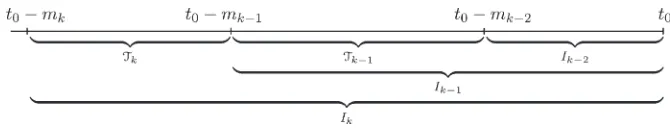
Figure 2. Local change point procedure. Choice of intervalsIkandTk:
and to a high delay in the reaction to changes in dependence measured by the parameterut.
To choose an interval of homogeneity, we use a local para-metric fitting approach as introduced by Polzehl and Spokoiny (2006), Belomestny and Spokoiny (2007) and Spokoiny (2009). The basic idea is to select for each time pointt0an intervalIt0¼ ½t0mt0;t0of lengthmt0in such a way that the time-varying copula parameter ut can be well approximated by a constant valueu. The question is, of course, how to select mt0in an online situation from historical data. The aim should be to selectIt0as close as possible to the so-called ‘‘oracle’’ choice interval. The oracle choice is defined as the largest interval I¼ ½t0mt0;t0, for which the small modeling bias condition
DIðuÞ ¼X
t2I
KðPut;PuÞ# D ð4:1Þ
for someD $0 holds. Here,u is constant andKðPq;Pq9Þ ¼ Eqlogfpðy;qÞ=pðy;q9Þg denotes the Kullback-Leibler diver-gence. In such an oracle choice interval, the parameterut0 ¼
utjt¼t0 can be ‘‘optimally’’ estimated from I¼ ½t0m
t0;t0. The error and risk bounds are calculated in Spokoiny (2009). It is important to mention that the concept of local parametric approximation allows one to treat in a unified way the case of ‘‘switching regime’’ models with spontaneous changes of parameters and the ‘‘smooth transition’’ case when the parameter varies smoothly in time.
The oracle choice of the interval of homogeneity depends on the unknown time-varying copula parameterut. The next sec-tion presents an adaptive (data-driven) procedure that mimics the oracle in the sense that it delivers the same accuracy of estimation as the oracle one. The trick is to find the largest interval in which the hypothesis of a local constant copula
parameter is supported. The local change point (LCP) detection procedure originates from Mercurio and Spokoiny (2004) and sequentially tests the hypothesis: ut is constant (i.e., ut ¼u) within some intervalI(local parametric assumption).
The LCP procedure for a given pointt0starts with a family of nested intervalsI0I1I2. . . IK¼IKþ1of the formIk¼ [t0mk,t0]. The sequencemkdetermines the length of these interval ‘‘candidates’’ (see Section 4.2). Every intervalIkleads to an estimate ~uk of the copula parameter ut0. The procedure selects one intervalI^out of the given family and, therefore, the corresponding estimate^u¼~u^
I.
The idea of the procedure is to screen each interval Tk¼
½t0mk;t0mk1sequentially and check each pointt2Tk
as a possible change point location (see Section 4.1 for more details). The family of intervals Ik and Tk are illustrated in
Figure 2. The interval Ik is accepted if no change point is detected withinT1;. . .;Tk. If the hypothesis of homogeneity
is rejected for an interval candidateIk, the procedure stops and selects the latest accepted interval. The formal description reads as follows:
Start the procedure withk¼1 and test the hypothesisH0,k of no structural changes within Tk using the larger testing
intervalIkþ1. If no change points were found inTk, thenIkis accepted. Take the next intervalTkþ1and repeat the previous
step until homogeneity is rejected or the largest possible intervalIK¼[t0mK,t0] is accepted. IfH0,kis rejected for
Tk, the estimated interval of homogeneity is the last accepted
intervalI^¼Ik1. If the largest possible intervalIKis accepted, we takeI^¼IK. We estimate the copula dependence parameter
u at time instant t0 from observations in I, assuming the^ homogeneous model within I^(i.e., we define ^ut0¼~uI^). We
also denote byI^kthe largest accepted interval afterksteps of
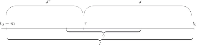
Figure 3. Homogeneity test. Testing intervalI, tested intervalT, and subintervalsJandJcfor a pointt2T:
Table 1. Critical valueszk(r;u*)
k
u*¼0.5 u*¼1.0 u*¼1.5
r¼0.2 r¼0.5 r¼1.0 r¼0.2 r¼0.5 r¼1.0 r¼0.2 r¼0.5 r¼1.0
1 3.64 3.29 2.88 3.69 3.29 2.84 3.95 3.49 2.96
2 3.61 3.14 2.56 3.43 2.91 2.35 3.69 3.02 2.78
3 3.31 2.86 2.29 3.32 2.76 2.21 3.34 2.80 2.09
4 3.19 2.69 2.07 3.04 2.57 1.80 3.14 2.55 1.86
5 3.05 2.53 1.89 2.92 2.22 1.53 2.95 2.65 1.49
6 2.87 2.26 1.48 2.92 2.17 1.19 2.83 2.04 0.94
7 2.51 1.88 1.02 2.64 1.82 0.56 2.62 1.79 0.31
8 2.49 1.72 0.35 2.33 1.39 0.00 2.35 1.33 0.00
9 2.18 1.23 0.00 2.03 0.81 0.00 2.10 0.60 0.00
10 0.92 0.00 0.00 0.82 0.00 0.00 0.79 0.00 0.00
NOTE: Critical values are obtained according to Equation (4.2), based on 5,000 simulations. Clayton copula,m0¼20 and
c¼1.25.
the algorithm and, by ^uk the corresponding estimate of the
copula parameter.
It is worth mentioning that the objective of the described estimation algorithm is not to detect the points of change for the copula parameter, but rather to determine the current dependence structure from historical data by selecting an interval of time homogeneity. This distinguishes our approach from other procedures for estimating a time-varying parameter by change point detection. A visible advantage of our approach is that it equally applies to the case of spontaneous changes in the dependence structure and in the case of smooth transition in the copula parameter. The obtained dependence structure can be used for different purposes in financial engineering, the most prominent being the calculation of the VaR (see also Section 6).
The theoretical results from Spokoiny and Chen (2007) and Spokoiny (2009) indicate that the proposed procedure provides the rate optimal estimation of the underlying parameter when this varies smoothly with time. It has also been shown that the procedure is very sensitive to structural breaks and provides the minimal possible delay in detection of changes, where the delay depends on the size of change in terms of Kullback-Leibler divergence.
4.1 Test of Homogeneity Against a Change
Point Alternative
In the homogeneity test against a change point alternative we want to check every point of an intervalT(recall Fig. 2), here
called the ‘‘tested interval,’’ on a possible change in the dependence structure at this moment. To perform this check, we assume a larger testing intervalIof formI¼[t0m,t0], so thatTis an internal subset withinI. The null hypothesisH0
means that"t2I,ut¼u(i.e., the observations inIfollow the
model with dependence parameteru). The alternative hypoth-esisH1claims that9t2Tsuch thatut¼u1fort2J¼[t,t0] andut¼u26¼u1fort2Jc¼[t0m,t) (i.e., the parameter
uchanges spontaneously in some pointt2T). Figure 3 depicts
I,T, and the subintervalsJandJcdetermined by the pointt2T.
Let LI(u) be the log-likelihood and ~uI the maximum
like-lihood estimate for the intervalI. The log-likelihood functions corresponding to H0and H1 are LI(u) and LJðu1Þ þLJcðu2Þ;
respectively. The likelihood ratio test for the single change point with known fixed locationtcan be written as
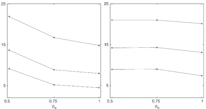
Figure 4. LCP and sudden jump in copula parameter. Pointwise median (full), and 0.25 and 0.75 quantiles (dotted) from^ut. True parameterut (dashed) withqa¼0.10,qb¼0.50, 0.75, and 1.00 (left, top to bottom); andqb¼0.10,qa¼0.50, 0.75, and 1.00 (right, top to bottom). Based on 100 simulations from Clayton copula, estimated with LCP,m0¼20,c¼1.25, andr¼0.5.
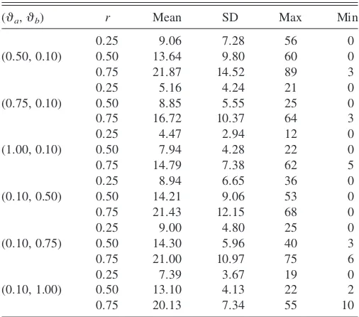
Table 2. Detection delay statistics
(qa,qb) r Mean SD Max Min
0.25 9.06 7.28 56 0
(0.50, 0.10) 0.50 13.64 9.80 60 0
0.75 21.87 14.52 89 3
0.25 5.16 4.24 21 0
(0.75, 0.10) 0.50 8.85 5.55 25 0
0.75 16.72 10.37 64 3
0.25 4.47 2.94 12 0
(1.00, 0.10) 0.50 7.94 4.28 22 0
0.75 14.79 7.38 62 5
0.25 8.94 6.65 36 0
(0.10, 0.50) 0.50 14.21 9.06 53 0
0.75 21.43 12.15 68 0
0.25 9.00 4.80 25 0
(0.10, 0.75) 0.50 14.30 5.96 40 3
0.75 21.00 10.97 75 6
0.25 7.39 3.67 19 0
(0.10, 1.00) 0.50 13.10 4.13 22 2
0.75 20.13 7.34 55 10
NOTE: The detection delaysdare calculated as in Equation (5.1), with the statistics based on 100 simulations. Clayton copula,m0¼20,c¼1.25, andr¼0.5. SD, standard deviation.
TI;t¼max
u1;u2 LJðu1Þ þLJ
cðu2Þ
f g max
u LIðuÞ ¼LJð~uJÞ þLJcð~uJcÞ LIð~uIÞ:
The test statistic for an unknown change point location is defined asTI ¼maxt2TTI;t. The change point test compares this test statistic with a critical valuezI;which may depend on the interval I. One rejects the hypothesis of homogeneity if TI >zI.
4.2 Parameters of the LCP Procedure
To apply the LCP testing procedure for local homogeneity, we have to specify some parameters. This includes selecting interval candidatesIkor, equivalently, tested intervalsTk and
choosing respective critical valueszk:One possible parameter set that has been used successfully in simulations is presented in the following section.
4.2.1 Selection of interval candidates Ikand internal points
Tk. It is useful to take the set of numbersmkdefining the length
ofIkandTkin the form of a geometric grid. We fix the value
m0and definemk¼[m0ck] fork¼1, 2,. . .,Kandc> 1 where [x] means the integer part ofx. We setIk¼[t0mk,t0] and
Tk¼ ½t0mk;t0mk1fork¼1, 2,. . .,K(see Fig. 2).
4.2.2 Choice of the critical valueszk: The algorithm is in
fact a multiple testing procedure. Mercurio and Spokoiny (2004) suggested selecting the critical value zk to provide the
overall first type error probability of rejecting the hypothesis of homogeneity in the homogeneous situation. Here we follow another proposal from Spokoiny and Chen (2007), which focuses on estimation losses caused by the ‘‘false alarm’’—in our case obtaining a homogeneity interval that is too small—rather than on its probability.
In the homogeneous situation withut[u* for allt2Ikþ1, the desirable behavior of the procedure is that after the firstk steps the selected intervalI^k coincides with Ikand the corre-sponding estimate^uk coincides with~uk, which means there is
no false alarm. On the contrary, in the case of a false alarm, the selected interval I^k is smaller than Ik and, hence, the corre-sponding estimate^ukhas larger variability than~uk. This means
that the false alarm during the early steps of the procedure is more critical than during the final steps, because it may lead to selecting an estimate with very high variance. The difference between ^uk and ~uk can naturally be measured by the value
LIkð~uk;^ukÞ ¼LIkð~ukÞ LIkð^ukÞ normalized by the risk of the
nonadaptive estimate ~uk, RðuÞ ¼maxk$1Eu LIkð~uk;u
Þ
1=2
. The conditions we impose read as
Eu LI kð~uk;^ukÞ
1=2
#rRðuÞ; k¼1;. . .;K; u2Q: ð4:2Þ The critical valueszkare selected as minimal values providing these constraints. In total we have K conditions to select K critical values z1;. . .;zK: The values zk can be selected
sequentially by Monte Carlo simulation, where one simulates under H0 : ut ¼ u*, "t 2 IK. The parameter r defines how conservative the procedure is. A smallr value leads to larger critical values and hence to a conservative and nonsensitive procedure, whereas an increase inrresults in more sensitive-ness at cost of stability. For details, see Spokoiny and Chen (2007) or Spokoiny (2009).
Figure 5. Divergences for upward and downward jumps. Kullback-Leibler divergences Kð0:10;qÞ (full) and Kðq;0:10Þ (dashed) for Clayton copula.
Figure 6. Mean detection delay and parameter jumps. Mean detection delays (dots) at ruler¼0.75, 0.50, and 0.25 from top to bottom. Left: qb¼0.10 (upward jump). Right:qa¼0.10 (downward jump), based on 100 simulations from Clayton copula,m0¼20,c¼1.25, andr¼0.5.
5. SIMULATED EXAMPLES
In this section we apply the LCP procedure on simulated data with a dependence structure given by the Clayton copula. We generate sets of six-dimensional data with a sudden jump in the dependence parameter given by (close to independence) and the other is set to larger values.
The LCP procedure is implemented with the family of interval candidates in form of a geometric grid defined bym0¼ 20 and c ¼ 1.25. The critical values, selected according to Equation (4.2) for differentrandu*, are displayed in Table 1. The choice ofu* has negligible influence in the critical values for fixedr, therefore we usez1;. . .;zKobtained withu*¼1.0.
Based on our experience, see Spokoiny and Chen (2007) and Spokoiny (2009), the default choice forris 0.5.
Figure 4 shows the pointwise median and quantiles of the estimated parameter^utfor distinct values of (qa,qb) based on 100 simulations. The detection delaydat ruler2[0, 1] to jump of sizeg¼utut1attis expressed by
dðt;g;rÞ ¼minfu $t: ^uu¼ut1þrgg t ð5:1Þ
and represents the number of steps necessary for the estimated
parameter to reach the r fraction of a jump in the true
parameter.
Detection delays are proportional to the probability of error of type II (i.e., the probability of accepting homogeneity in case of a jump). Thus, tests with higher power correspond to lower delaysd. Moreover, because the Kullback-Leibler divergences for upward and downward jumps are proportional to the power of the respective homogeneity tests, larger divergences result in faster jump detections.
The descriptive statistics for detection delays to jumps att¼ 11 for different values of (qa,qb) are in Table 2. The mean detection delay decreases withg¼qbqaand are higher for downward jumps than for upward jumps. Figure 5 shows that for Clayton copulae the Kullback-Leibler divergence is higher for upward jumps than for downward jumps. Figure 6 displays the mean detection delays against jump size for upward and downward jumps.
The LCP procedure is also applied on simulated data with smooth transition in the dependence parameter given by
ut¼
Figure 7 depicts the pointwise median and quantiles of the estimated parameter^utand the true parameterutfor (qa,qb) set to (0.10, 1.00) and (1.00, 0.10).
6. EMPIRICAL RESULTS
In this section the VaR from German stock portfolios is
estimated based on time-varying copulae and RiskMetrics
approaches. The time-varying copula parameters are selected by local change point (LCP) and moving window procedures. Backtesting is used to evaluate the performances of the three methods in VaR estimation.
Two groups of six stocks listed on DAX are used to compose the portfolios. Stocks from group 1 belong to three different industries: automotive (Volkswagen and DaimlerChrysler), insurance (Allianz and Mu¨nchener Ru¨ckversicherung), and chemical (Bayer and BASF). Group 2 is composed of stocks from six industries: electrical (Siemens), energy (E.ON), metal-lurgical (ThyssenKrupp), airlines (Lufthansa), pharmaceutical (Schering), and chemical (Henkel). The portfolio values are calculated using 1,270 observations, from January 1, 2000 to December 31, 2004, of the daily stock prices (data available at http://sfb649.wiwi.hu-berlin.de/fedc).
The selected copula belongs to the Clayton family (Eq. 2.3). Clayton copulae have a natural interpretation and are well advocated in risk management applications. In line with the stylized facts for financial returns, Clayton copulae are asym-metric and present lower tail dependence, modeling joint Figure 7. LCP and smooth change in copula parameter. Pointwise median (full), 0.25 and 0.75 quantiles (dotted) from^utand true parameterut (dashed) withqa¼0.10 andqb¼1.00 (left), andqa¼1.00 andqb¼0.10 (right). Based on 100 simulations from Clayton copula, estimated with LCP,m0¼20,c¼1.25, andr¼0.5.
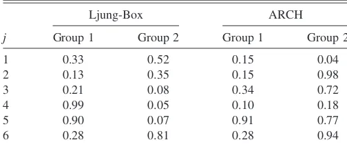
Table 3.pValues from tests on residuals^et;j
j
Ljung-Box ARCH
Group 1 Group 2 Group 1 Group 2
1 0.33 0.52 0.15 0.04
extreme events at lower orthants with higher probability than Gaussian copulae for the same correlation, see McNeil, Frey, and Embrechts (2005). This fact is essential for VaR calcu-lations and is illustrated by the ratio between Equations (2.2) and (2.3) for off-diagonal elements ofCset to 0.25 andu ¼ 0.5. For the quantiles ui ¼ 0.05, i ¼ 1, . . ., 6 the ratio CGaCðu1;. . .;u6Þ=Cuðu1;. . .;u6Þequals 2.33102, whereas for
the 0.01 quantiles it equals 1.33103.
The VaR estimation follows the steps described in Section 3. Using theRiskMetricsapproach, the log-returnsXtare assumed
conditionally normal distributed with zero mean and covari-ance matrix following a GARCH specification with fixed decay factorl¼0.94 as in Equation (3.4).
In the time-varying copulae estimation, the log-returns are modeled as in Equation (3.5), where the innovations et have
cdfFt;etðx1;. . .;xdÞ ¼CutfFt;1ðx1Þ;. . .;Ft;dðxdÞgandCuis the Clayton copula. The univariate log-returnsXt,jcorresponding to stockjare devolatized according to RiskMetrics(i.e., with zero conditional means and conditional variancess2
t;jestimated
by the univariate version of Equation (3.4) with a decay factor equal to 0.94). We note that this choice sets the same specifi-cation for the dynamics of the univariate returns across all methods (RiskMetrics, moving windows, and LCP), making their performances in VaR estimation comparable. Moreover, as the means from daily returns are clearly dominated by the variances and are approximately independent on the available information sets (see Jorion 1995; Fleming, Kirby, and Ostdiek 2001; and Christoffersen and Diebold 2006), their specification is very unlikely to cause a perceptible bias in the estimated variances and dependence parameters. Therefore, the zero mean assumption is, as pointed out by Kim, Malz, and Mina (1999), as good as any other choice. Daily returns are also modeled with zero conditional means in Fan and Gu (2003) and Ha¨rdle, Herwartz, and Spokoiny (2003) among others.
The GARCH specification (Eq. 3.4) withl¼0.94 optimizes variance forecasts across a large number of assets (Morgan 1996), and is widely used in the financial industry. Different choices for the decay factor (like 0.85 or 0.98) result in negligible changes (about 3%) in the estimated dependence parameter.
Thepvalues from the Ljung-Box test for serial correlation and from Autoregressive Conditional Heteroscedasticity (ARCH) test for heteroscedasticity effects in the obtained residuals^et;jare in Table 3. Normality is rejected by Jarque-Bera test, withpvalues approximately 0.00 for all residuals in both groups. The empirical cummulative distribution functions of residuals as defined in Equation (2.4) are used for the copula estimation.
With the moving windows approach, the size of the esti-mating window is fixed as 250 days corresponding to 1 busi-ness year (the same size is used in, for example, Fan and Gu (2003)). For the LCP procedure, following Section 4.2, we set the family of interval candidates as a geometric grid withm0¼ 20,c¼1.25, andr ¼0.5. We have chosen these parameters from our experience in simulations (for details on robustness of the reported results with respect to the choice ofm0andc,refer to Spokoiny (2009)).
The performance of the VaR estimation is evaluated based on backtesting. At each timet,the estimated VaR at levelafor a portfoliowis compared with the realization ltof the
corre-sponding P&L function (see Eq. 3.2), with an exceedance occurring for eachltless thanVaRdtðaÞ:The ratio of the number
of exceedances to the number of observations gives the exceedance ratio
^
awðaÞ ¼
1 T
XT t¼1 1
flt<dVaRtðaÞg
:
Because the first 250 observations are used for estimation,T¼ 1,020. The difference between ^a and the desired level a is expressed by the relative exceedance error
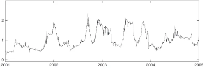
Figure 8. Time-varying dependence, group 1. Copula parameter^utestimated with LCP method, Clayton copula,m0¼20,c¼1.25, andr¼0.5.
Figure 9. Time-varying dependence, group 2. Copula parameter^utestimated with LCP method, Clayton copula,m0¼20,c¼1.25, andr¼0.5.
ew¼ ða^aÞ=a:
We compute exceedance ratios and relative exceedance errors to levelsa¼0.05 and 0.01 for a setW ¼{w*,wn;n¼1,. . .,
100} of portfolios, where eachwn¼ ðwn;1;. . .;wn;6Þ>is a
rea-lization of a random vector uniformly distributed on S ¼
fðx1;. . .;x6Þ 2R6:P 6
i¼1xi¼1;xi $0:1g;andw ¼1=6I6,
with Id denoting the (d 3 1) vector of ones, is the equally
weighted portfolio. The degree of diversification of a portfolio can be measured based on the majorization preordering onS (see Marshall and Olkin 1979). In other words, a portfoliowais
more diversified than portfolio wb if wawb: Under the
majorization preordering the vectorw* satisfiesw wfor all w 2 S; therefore, the equally weighted portfolio is the most
diversified portfolio fromW, see Ibragimov and Walden (2007).
The average relative exceedance error over portfolios and the corresponding standard deviation
AW ¼ 1 jWj
X
w2W
ew
DW ¼ 1 jWj
X
w2W
ðewAWÞ2
( )1
2
are used to evaluate the performances of the time-varying copulae andRiskMetricsmethods in VaR estimation.
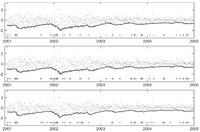
The dependence parameter estimated with LCP for stocks from groups 1 and 2 are shown in Figures 8 and 9. The different industry concentrations in each group are reflected in the higher parameter values obtained for group 1. The P&L and the VaR at level 0.05 estimated with LCP, moving windows, and Figure 10. Estimated VaR across methods, group 1. P&L realizationslt(dots),VaRtd ðaÞ(line), and exceedance times (crosses). Estimated with LCP (top), moving windows (middle), andRiskMetrics(bottom) for equally weighted portfoliow* at levela¼0.05.
Figure 11. Estimated VaR across methods, group 2. P&L realizationslt(dots),VaRtd ðaÞ(line), and exceedance times (crosses). Estimated with LCP (top), moving windows (middle), andRiskMetrics(bottom) for equally weighted portfoliow* at levela¼0.05.
RiskMetricsmethods for the equally weighted portfoliow* are
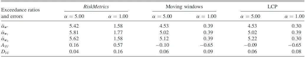
in Figures 10 (group 1) and 11 (group 2). Exceedance ratios for portfoliosw*,w1, andw2; average relative exceedance errors;
and corresponding standard deviations across methods and levels are shown in Tables 4 (group 1) and 5 (group 2).
Based on the exceedance errors, the LCP procedure
out-performs the moving windows (second best) andRiskMetrics
methods in VaR estimation in group 1. At level 0.05, the average error associated with copula methods is about half
the error from RiskMetrics estimation for nearly the same
standard deviation. At level 0.01, the LCP average error is the smallest in absolute value, and copula methods present less standard deviations. At this level, copula methods
over-estimate VaR, and RiskMetrics underestimates it. Although
overestimation of VaR means that a financial institution would be requested to keep more capital aside than necessary to guarantee the desired confidence level, underestimation means that less capital is reserved and the desired level is not guaranteed. Therefore, from the regulatory point of view, overestimation is preferred to underestimation. In the less con-centrated group 2, LCP outperforms moving windows and RiskMetrics at the level 0.05, presenting the smallest average error in magnitude for nearly the same value ofDW. At level
0.01, copula methods overestimate and RiskMetrics
under-estimates the VaR by about 60%.
It is interesting to note the effect of portfolio diversification on the exceedance errors for group 1 and level 0.01. The errors decrease with increasing portfolio diversification for copulae methods but become larger under theRiskMetricsestimation. For other groups and levels, the diversification effects are not clear. Refer to Ibragimov (2007) and Ibragimov and Walden (2007) for details on the effects of portfolio diversification under heavy-tailed distributions in risk management.
7. CONCLUSION
In this article we modeled the dependence structure from German equity returns using time-varying copulae with adap-tively estimated parameters. In contrast to Patton (2006) and Rodriguez (2007), we neither specified the dynamics nor assumed regime switching models for the copula parameter. The parameter choice was performed under the local homo-geneity assumption with homohomo-geneity intervals recovered from the data through local change point analysis.
We used time-varying Clayton copulae, which are asym-metric and present lower tail dependence, to estimate the VaR from portfolios of two groups of German securities, presenting different levels of industry concentration.RiskMetrics, a widely used methodology based on multivariate normal distributions, was chosen as a benchmark for comparison. Based on back-testing, the adaptive copula achieved the best VaR estimation performance in both groups, with average exceedance errors mostly small in magnitude and corresponding to sufficient capital reserve for covering losses at the desired levels.
The better VaR estimates provided by Clayton copulae indicate that the dependence structure from German equities may contain nonlinearities and asymmetries, such as stronger dependence at lower tails than at upper tails, that cannot be captured by the multivariate normal distribution. This asym-metry translates into extremely negative returns being more correlated than extremely positive returns. Thus, our results for the German equities resemble those from Longin and Solnik (2001), Ang and Chen (2002) and Patton (2006) for interna-tional markets, U.S. equities, and Deutsch mark/Japanese yen exchange rates, where empirical evidence for asymmetric dependences with increasing correlations in market downturns were found.
Table 4. Exceedance ratios and errors, group 1
Exceedance ratios
NOTE: Exceedance ratios for portfoliosw*,w1, andw2, and average and standard deviation from relative exceedance errors. Across levels and methods, ratios and levels are expressed as a percentage.
Table 5. Exceedance ratios and errors, group 2
Exceedance ratios
NOTE: Exceedance ratios for portfoliosw*,w1, andw2, and average and standard deviation from relative exceedance errors. Across levels and methods, ratios and levels are expressed as a percentage.
Furthermore, in the Gaussian framework, with non-linearities and asymmetries taken into consideration through the use of Clayton copulae, the adaptive estimation produces better VaR fits than the moving window estimation. The high sensitive adaptive procedure can capture local changes in the dependence parameter that are not detected by the estimation with a scrolling window of fixed size.
The main advantage of using time-varying copulae to model dependence dynamics is that the normality assumption is not needed. With the proposed adaptively estimated time-varying copulae, neither normality assumption nor specification for the dependence dynamics are necessary. Hence, the method provides more flexibility in modeling dependences between markets and economies over time.
ACKNOWLEDGMENTS
Financial support from theDeutsche Forschungsgemeinschaft viaSFB 649‘‘O¨ konomisches Risiko,’’ Humboldt-Universita¨t zu Berlin is gratefully acknowledged. The authors also thank the editor, an associate editor, and two referees for their helpful comments.
[Received October 2006. Revised November 2007.]
REFERENCES
Andrews, D. W. K. (1993), ‘‘Tests for Parameter Instability and Structural Change With Unknown Change Point,’’Econometrica,61, 821–856. Andrews, D. W. K., and Ploberger, W. (1994), ‘‘Optimal Tests When a
Nui-sance Parameter Is Present Only Under the Alternative,’’Econometrica,62, 1383–1414.
Ang, A., and Chen, J. (2002), ‘‘Asymmetric Correlations of Equity Portfolios,’’ Journal of Financial Economics,63, 443–494.
Belomestny, D., and Spokoiny, V. (2007), ‘‘Spatial Aggregation of Local Likelihood Estimates With Applications to Classification,’’The Annals of Statistics,35, 2287–2311.
Chen, X., and Fan, Y. (2006), ‘‘Estimation and Model Selection of Semi-parametric Copula-Based Multivariate Dynamic Models Under Copula Misspecification,’’Journal of Econometrics,135, 125–154.
Chen, X., Fan, Y., and Tsyrennikov, V. (2006), ‘‘Efficient Estimation of Semi-parametric Multivariate Copula Models,’’Journal of the American Statistical Association,101, 1228–1240.
Cherubini, U., Luciano, E., and Vecchiato, W. (2004),Copula Methods in Finance, Chichester: Wiley.
Christoffersen, P., and Diebold, F. (2006), ‘‘Financial Asset Returns, Direction-of-Change Forecasting, and Volatility Dynamics,’’Management Science,52, 1273–1287.
Cont, R. (2001), ‘‘Empirical Properties of Asset Returns: Stylized Facts and Statistical Issues,’’Quantitative Finance,1, 223–236.
Embrechts, P., Hoeing, A., and Juri, A. (2003a), ‘‘Using Copulae to Bound the Value-at-Risk for Functions of Dependent Risks,’’Finance and Stochastics, 7, 145–167.
Embrechts, P., Lindskog, F., and McNeil, A. (2003b), ‘‘Modelling Dependence with Copulas and Applications to Risk Management,’’ inHandbook of Heavy Tailed Distributions in Finance, ed. S. Rachev, Amsterdam: North-Holland, pp. 329–384.
Embrechts, P., McNeil, A., and Straumann, D. (2002), ‘‘Correlation and Dependence in Risk Management: Properties and Pitfalls,’’ inRisk Man-agement: Value at Risk and Beyond, ed. M. Dempster, Cambridge, UK: Cambridge University Press.
Fan, J., and Gu, J. (2003), ‘‘Semiparametric Estimation of Value-at-Risk,’’The Econometrics Journal,6, 261–290.
Fleming, J., Kirby, C., and Ostdiek, B. (2001), ‘‘The Economic Value of Vol-atility Timing,’’The Journal of Finance,56, 239–354.
Franke, J., Ha¨rdle, W., and Hafner, C. (2004),Statistics of Financial Markets, Heidelberg: Springer-Verlag.
Fre´chet, M. (1951), ‘‘Sur les Tableaux de Correlation Dont les Marges Sont Donne´es,’’Annales de l’Universite´ de Lyon, Sciences Mathe´matiques et Astronomie,14, 5–77.
Giacomini, E., and Ha¨rdle, W. (2005), ‘‘Value-at-Risk Calculations With Time Varying Copulae,’’ in Bulletin of the International Statistical Institute, Proceedings of the 55th Session.
Granger, C. (2003), ‘‘Time Series Concept for Conditional Distributions,’’ Oxford Bulletin of Economics and Statistics,65, 689–701.
Hansen, B. E. (2001), ‘‘The New Econometrics of Structural Change: Dating Breaks in U.S. Labor Productivity,’’The Journal of Economic Perspectives, 15, 117–128.
Ha¨rdle, W., Herwartz, H., and Spokoiny, V. (2003), ‘‘Time Inhomogeneous Multiple Volatility Modelling,’’Journal of Financial Econometrics,1, 55–95. Ha¨rdle, W., Kleinow, T., and Stahl, G. (2002),Applied Quantitative Finance,
Springer-Verlag, Heidelberg.
Hoeffding, W. (1940), ‘‘Maßstabinvariante Korrelationstheorie,’’Schriften des mathematischen Seminars und des Instituts fu¨r angewandte Mathematik der Universita¨t Berlin,5, 181–233.
Hu, L. (2006), ‘‘Dependence Patterns Across Financial Markets: A Mixed Copula Approach,’’Applied Financial Economics,16, 717–729.
Ibragimov, R. (2007), ‘‘Efficiency of Linear Estimators Under Heavy-Tailed-ness: Convolutions ofa-Symmetric Distributions,’’Econometric Theory,23, 501–517.
Ibragimov, R., and Walden, J. (2007), ‘‘The Limits of Diversification When Losses May be Large,’’Journal of Banking and Finance,31, 2551–2569. Joe, H. (1997), Multivariate Models and Dependence Concepts, London:
Chapman & Hall.
Jorion, P. (1995), ‘‘Predicting Volatility in the Foreign Exchange Market,’’The Journal of Finance,50, 507–528.
Morgan, J. P. (1996),RiskMetrics Technical Document, New York: RiskMetrics Group.
Kim, J., Malz, A. M., and Mina, J. (1999),Long Run Technical Document, New York: RiskMetrics Group.
Longin, F., and Solnik, B. (2001), ‘‘Extreme Correlation on International Equity Markets,’’The Journal of Finance,56, 649–676.
Mari, D., and Kotz, S. (2001),Correlation and Dependence, London: Imperial College Press.
Marshall, A., and Olkin, I. (1979),Inequalities: Theory of Majorizations and Its Applications, New York: Academic Press.
McNeil, A. J., Frey, R., and Embrechts, P. (2005),Quantitative Risk Management: Concepts, Techniques and Tools, Princeton, NJ: Princeton University Press. Mercurio, D., and Spokoiny, V. (2004), ‘‘Estimation of Time Dependent
Vol-atility via Local Change Point Analysis With Applications to Value-at-Risk,’’ Annals of Statistics,32, 577–602.
Nelsen, R. (1998),An Introduction to Copulas, New York: Springer-Verlag. Patton, A. (2004), ‘‘On the Out-of-Sample Importance of Skewness and
Asymmetric Dependence for Asset Allocation,’’ Journal of Financial Econometrics,2, 130–168.
——— (2006), ‘‘Modelling Asymmetric Exchange Rate Dependence,’’ Inter-national Economic Review,47, 527–556.
Perron, P. (1989), ‘‘The Great Crash, the Oil Price Shock and the Unit Root Hypothesis,’’Econometrica,57, 1361–1401.
Polzehl, J., and Spokoiny, V. (2006), ‘‘Propagation–Separation Approach for Likelihood Estimation,’’Probability Theory and Related Fields,135, 335–362. Quintos, C., Fan, Z., and Philips, P. C. B. (2001), ‘‘Structural Change Tests in Tail Behaviour and the Asian Crisis,’’The Review of Economic Studies,68, 633–663.
Rodriguez, J. C. (2007), ‘‘Measuring Financial Contagion: A Copula Approach,’’Journal of Empirical Finance,14, 401–423.
Sklar, A. (1959), ‘‘Fonctions de Re´partition a`nDimensions et Leurs Marges,’’ Publications de l’Institut de Statistique de l’Universite de Paris,8, 229–231. Spokoiny, V. (2009),Local Parametric Methods in Nonparametric Estimation,
Berlin, Heidelberg: Springer-Verlag.
Spokoiny, V., and Chen, Y. (2007),Multiscale Local Change Point Detection with Applications to Value-at-Risk,Preprint 904, Berlin: Weierstrass Institute Berlin.
Stock, J.H. (1994), ‘‘Unit Roots, Structural Breaks and Trends,’’ inHandbook of Econometrics,Vol. 4, ed. R. F. Engle and D. McFadden, Amsterdam: North-Holland, pp. 2739–2841.
Zivot, E., and Andrews, D. W. K. (1992), ‘‘Further Evidence on the Great Crash, the Oil Price Shock and the Unit Root Hypothesis,’’Journal of Business & Economic Statistics,10, 251–270.