103 FACE RECOGNITION USING COMPLEX VALUED BACKPROPAGATION Z Nafisah1 , Muhammad Febrian Rachmadi2 , and E M Imah1

(1)

103 FACE RECOGNITION USING COMPLEX VALUED BACKPROPAGATION

Z Nafisah

1

_{, Muhammad Febrian Rachmadi}

2

_{, and E M Imah}

1*

1

_{Mathematics Department, Faculty of Mathematics and Natural Sciences, Universitas Negeri Surabaya}

Jl. Ketintang, Surabaya, 60231, Indonesia

2

_{School of Informatics, The University of Edinburgh, 11 Crichton Street, Edinburgh EH8 9LE, United}

Kingdom

*E-mail: [email protected]

Abstract

Face recognition is one of biometrical research area that is still interesting. This study

discusses the Complex-Valued Backpropagation algorithm for face recognition.

Complex-Valued Backpropagation is an algorithm modified from Real-Valued

Backpropagation algorithm where the weights and activation functions used are complex.

The dataset used in this study consist of 250 images that is classified in 5 classes. The

performance of face recognition using Complex-Valued Backpropagation is also

compared with Real-Valued Backpropagation algorithm. Experimental results have

shown that Complex-Valued Backpropagation accuracy is better than Real-Valued

Backpropagation.

Keywords: Face Recognition, Complex Valued Backpropagation

Abstrak

Pengenalan wajah seseorang merupakan salah satu riset di bidang biometrika yang masih

sangat menarik hingga saat ini. Dalam penelitian ini membahas algoritma

Complex

Valued Backpropagation untuk pengenalan wajah.

Complex Valued Backpropagation

merupakan algoritma yang dikembangkan dari algoritma

Real Valued Backpropagation

dimana bobot dan fungsi aktivasi yang digunakan bernilai kompleks. Dataset yang

digunakan berjumlah 250 citra wajah yang diklasifikasikan kedalam 5 kelas. Performa

hasil pengenalan wajah menggunakan

Complex Valued backpropagation juga

dibandingkan dengan algoritma

Real Valued Backpropagation. Hasil eksperimen yang

telah dilakukan menunjukkan bahwa akurasi Complex Valued Backpropagation lebih baik

dibandingkan dengan Real Valued Backpropagation.

Kata Kunci: Pengenalan Wajah, Complex Valued Backpropagation

1. Introduction

Face recognition is one of the biometrical research.

Until todays face recognition still interesting and

challenging research area. Face recognition

already using in many applications such as

security sys-tems, credit card verification,

criminal identifi-cation etc. Recently, there are

many methods and algorithms that is used for face

recognition such as Chittora et al using support

vector machine [1], Kathirvalavakumar et al using

Wavelet Packet Coefficients and RBF network [2],

Cho et al using PCA and GABOR wavelets [3],

Sharma using PCA and SVM [4]. Almost all those

authors studying face recognition using Real

Valued Machine Learning.

(2)

advantages in reducing the number of parameters

and operations involved. In addtion, CVNN has

computational advantages over real valued neural

networks in solving classification problems [6].

Several literatures was use CVNN such as: A

Novel Diagnosis System for Parkinson’s Disease

Using Complex-Valued Artificial Neural Network

with

k-Means

Clustering

Feature

[7],

Fluorescence Microscopy Images Recognition

using Complex CNN [8], A New Automatic

Method of Parkinson Disease Identification Using

Complex-Valued Neural Network [9], Automatic

Sleep Stage Classification of Single-Channel EEG

by Using Complex-Valued Convolutional Neural

Network [10].

One of the learning processes that utilizes

Complex valued neural network is Complex

Valued backpropagation (CVBP). CVBP is an

algorithm developed from Real Valued

Backpro-pagation algorithm where the weights and

acti-vation functions used are complex. According to

research conducted by Zimmerman, the average

learning speed of the CVBP algorithm is better

than the Real Valued backpropagation (RVBP)

[11]. Based on that literature, this study will

discuss the performace comparison between

Com-plex Valued Backpropagation (CVBP) algorithm

and Real Valued Backpropagation (RVBP)

algorithm for face recognition. This study already

modified the converting process from complex

value in hidden layer to real value in output layer

using complex modulus, then the complex

modulus is using as input variable in activation

function. This process is more simple than CVBP

that proposed by Zimmerman, because CVBP that

proposed by Zimmerman is still using complex

value until its mapping into output classes.

This paper is organized as follows: Section II

describes the classification process using Real

Valued backpropagation (RVBP) and Complex

Valued Backpropagation (CVBP). The

experi-mental results are given in Section III. Finally,

section IV is present the conclusion of the study.

2. Methods

Feature Extraction

Principal component analysis (PCA) is a feature

extraction technique that can reduce data

dimen-sions without losing important information in the

data [4]. In PCA face recognition system, every

face image is represented as a vector [12]. Let

there are N face images and each image

𝑋

_𝑖

is a

2-dimensional array of size mxn of intensity values.

An image

𝑋

_𝑖

can be converted into a vector of B

(B=mxn) pixels, where,

𝑋

_𝑖

= (𝑥

_𝑖1

, 𝑥

_𝑖2

, … , 𝑥

_𝑖𝐵

)

.

Define the training set of

N images by

𝑋 =

(𝑋

1

, 𝑋

2

, … , 𝑋

𝑁

) ⊂ ℜ

𝐵𝑥𝑁

. The covariance matrix is

defined in Eq. 1.

𝐶 =

_𝑁−11

∑ (𝑋

𝑁𝑖=1 𝑖

− 𝑋̅)

(𝑋

𝑖

− 𝑋̅)

𝑇

(1)

where

𝑋̅ =

1

𝑁

∑ 𝑋

𝑁𝑖=1 𝑖

is the mean image of the

training set. Then, the eigenvalues and

eigen-vectors are calculated from the covariance matrix

𝐶

. Let

𝑄 = (𝑄

₁

, 𝑄

₂

, … , 𝑄

_𝑟

) ⊂ ℜ

𝐵𝑥𝑁

(𝑟 < 𝑁)

be

the

r eigenvectors corresponding to

r largest

non-zero eigenvalues. Each of the

r eigenvectors is

called an eigenface. Now, each of the face images

of the training set

𝑋

_𝑖

is projected into the

eigenface space to obtain its corresponding

eigenface-based feature

𝑍

_𝑖

⊂ ℜ

𝑟𝑥𝑁

, which is

defined in Eq. 2.

𝑍

𝑖

= 𝑄

𝑇

𝑌

𝑖

, 𝑖 = 1,2, … , 𝑁

(2)

where

𝑌

_𝑖

is the mean-subtracted image of

𝑋

_𝑖

.

Classification

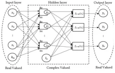
Real Valued Backpropagation (RVBP)

Real Valued Backpropagation is models of

multi-ple layer network where the weights and

Figure 1. The Real Valued Backpropagation architecture

model

(3)

activation function used are real [13]. RVBP is a

supervised learning algorithm, both input and

target output vectors are provided for training the

network [14]. The error data at the output layer is

calculated using network output and target output.

Then the error is back propagated to intermediate

layers, allowing incoming weights to these layers

to be updated [15]. Figure 1 shows RVBP model.

The input, weights, threshold, and output

signals are a real number. The activity of the

neuron

𝑧

_𝑝

and

𝑦

_𝑚

is defined in Eq. 3 and Eq. 4.

𝑧

𝑝

= ∑ 𝑣

𝑛 𝑝𝑛

𝑥

𝑛

+ 𝑏

𝑝

(3)

𝑦

𝑚

= ∑ 𝑤

𝑝 𝑚𝑝

𝑧

𝑝

+ 𝐼

𝑚

(4)

where

𝑣

_𝑝𝑛

and

𝑤

_𝑚𝑝

are real valued weight

con-necting neuron

m and

p,

𝑥

_𝑛

is the input signal

from neuron n,

𝑧

_𝑝

is the input signal from neuron

p, and

𝑏

_𝑝

,

𝐼

_𝑚

are the real valued threshold value

of neuron

p and

m. To obtain the output signal,

the activity value

𝑦

_𝑚

is defined in Eq. 5.

𝑓

𝑅

(𝑦) = 1/(1 + exp(−𝑦))

(5)

where the function above is called the sigmoid

binary function. For the sake of simplicity, the

networks used both in the analysis and

experiments will have three layers. We will use

𝑉

𝑝𝑛

for the weight between the input neuron n and

the hidden neuron p,

𝑊

_𝑚𝑝

for the weight between

the hidden neuron p and the output neuron m,

𝐵

_𝑝

for the threshold of the hidden neuron

𝐵

_𝑝

, and

𝐼

_𝑚

for the threshold of the output neuron

m. Let

𝑋

_𝑛

,

𝐻

𝑝

,

𝑂

𝑚

denote the output values of the input

neuron

n, the hidden neuron

p, and the output

neuron m, respectively. Let also

𝑈

_𝑝

and

𝑆

_𝑚

denote

the internal potentials of the hidden neuron p and

the output neuron m, respectively.

𝑈

_𝑝

,

𝑆

_𝑚

,

𝐻

_𝑝

,

𝑂

_𝑚

can be defined respectively as

𝑈

_𝑝

= ∑ 𝑉

_𝑛 _𝑝𝑛

𝑋

_𝑛

+

𝐵

𝑝

,

𝑆

𝑚

= ∑ 𝑊

𝑝 𝑚𝑝

𝐻

𝑝

+ 𝐼

𝑚

,

𝐻

𝑝

= 𝑓

𝑅

(𝑈

𝑝

)

, and

𝑂

𝑚

= 𝑓

𝑅

(𝑆

𝑚

)

. Let

𝛿

𝑚

= 𝑇

𝑚

− 𝑂

𝑚

denoted the

error between the actual pattern

𝑂

_𝑚

and the target

pattern

𝑇

_𝑚

of output neuron

m. The real valued

neural network error is defined by the following

Eq. 6.

𝐸 =

1₂

∑

𝑁

(

𝑚=1

𝑇

𝑚

− 𝑂

𝑚

)

2

(6)

where N is the number of output neurons.

Next, we define a learning rule for RVBP

model described above. We can show that the

weights and the thresholds should be updated

according to the following Eq. 7 and Eq.8.

∆𝑊

𝑚𝑝

= −𝛼.

_𝜕𝑊𝜕𝐸_𝑚𝑝

(7)

∆𝑉

𝑝𝑛

= −𝛼.

_𝜕𝑉𝜕𝐸_𝑝𝑛

(8)

where

𝛼

is learning rate. Equation can be

express-ed in Eq. 9 and Eq. 10.

∆𝑊

𝑚𝑝

= 𝛼(𝛿

𝑚

(1 − 𝑂

𝑚

)𝑂

𝑚

) 𝐻

𝑝

(9)

∆𝑉

𝑚𝑙

= ((1 − 𝐻

𝑝

)𝐻

𝑝

× ∑ 𝛿

𝑁 𝑚

(1 −

𝑂

𝑚

)𝑂

𝑚

𝑊

𝑚𝑝

) 𝑋

𝑛

(10)

The algorithm of RVBP can be written as

follows: (1) Initialization, set all weights and

thresholds with a random real number; (2)

Presentation of input and desired outputs (target),

present the input vector

𝑥

₁

, 𝑥

₂

, . . . , 𝑥

_𝑁

and

corresponding desired target

𝑡

₁

, 𝑡

₂

, . . . , 𝑡

_𝑁

one pair

at a time, where N is the total number of training

patterns; (3) Calculation of actual outputs, use the

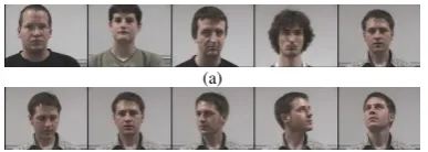
(a)

(b)

Figure 3. (a) Original face image of five persons (b) Original face image with various position

Figure 4. The result of pre-processing image

(a) (b) (c) (d) (e) (f)

(4)

formula in Eq. (3-5) To calculate output signals;

(4) Updates of weights and thresholds, use the

formulas in Eq. (9-10) To calculate adapted

weights and thresholds.

Complex Valued Backpropagation (CVBP)

Complex Valued Backpropagation is an algorithm

developed from Real Valued Backpropagation

where the weights and activation function used

are complex [16]. The goal of CVBP is to

minimize the aproximation error. Several kinds of

literature that compare CVBP and RVBP often

conclude that CVBP is better than RVBP . This

research will also prove some statement best

algorithm CVBP modelling than RVBP modelling.

Figure 2 shows a CVBP model.

The input and output signals in this study are

a real number, while weights, threshold, and

complex number consisting of real and imaginary

parts is defined in Eq. 13.

simplicity, the networks used both in the analysis

and experiments will have three layers. We will

defined by the following Eq.15[11].

𝐸 =

1₂

∑

𝑁

(

𝑛=1

𝑇

𝑛

− 𝑂

𝑛

)(𝑇

̅̅̅̅̅̅̅̅̅̅̅̅

𝑛

− 𝑂

𝑛

)

(15)

where N is the number of output neurons.

Next, we define a learning rule for CVBP

model described above. We can show that the

weights and the thresholds should be updated

according to the following Eq. 16 and Eq. 17[18].

∆𝑊

𝑛𝑚

= −𝛼.

_{𝜕𝑅𝑒[𝑊}𝜕𝐸

Architecture 1 hidden layer

Hidden Neuron 5, 50, 100, 150, and 200 Neuron Output 5 (Classification of face

recognition)

RESULTS WITH VARIOUS HIDDEN NEURON

Hidden Neuron Accuracy (%)

RVBP CVBP

RESULTS WITH VARIOUS LEARNING RATE

Learning rate Accuracy (%)

(5)

where

𝛼

is learning rate. Equation can be

expres-sed in Eq. 18 and Eq. 19.

∆𝑊

𝑛𝑚

= 𝛼(𝑅𝑒[𝛿

𝑛

](1 − 𝑅𝑒[𝑂

𝑛

])𝑅𝑒[𝑂

𝑛

] +

𝑖. 𝐼𝑚[𝛿

𝑛

_{](1 − 𝐼𝑚[𝑂}

𝑛

])𝐼𝑚[𝑂

𝑛

])𝐻

̅̅̅̅

𝑚

(18)

∆𝑉𝑚𝑙=

𝛼

(

(1 − 𝑅𝑒[𝐻𝑚])𝑅𝑒[𝐻𝑚] ×

∑ ( 𝑅𝑒[𝛿𝑛](1 − 𝑅𝑒[𝑂𝑛])𝑅𝑒[𝑂𝑛]𝑅𝑒[𝑊𝑛𝑚]

+𝐼𝑚[𝛿𝑛_{](1 − 𝐼𝑚[𝑂}

𝑛])𝐼𝑚[𝑂𝑛]𝐼𝑚[𝑊𝑛𝑚]) 𝑁

−𝑖 (1 − 𝐼𝑚[𝐻𝑚])𝐼𝑚[𝐻𝑚] ×

∑ ( 𝑅𝑒[𝛿𝑛](1 − 𝑅𝑒[𝑂𝑛])𝑅𝑒[𝑂𝑛]𝐼𝑚[𝑊𝑛𝑚]

−𝐼𝑚[𝛿𝑛_{](1 − 𝐼𝑚[𝑂}

𝑛])𝐼𝑚[𝑂𝑛]𝑅𝑒[𝑊𝑛𝑚])

𝑁 ₎

𝑋̅ 𝑙

(19)

where

𝑧̅

denotes the complex conjugate of

complex number

𝑧

.

The algorithm of CVBP can be written as

follows: (1) Initialization, set all weights and

thresholds with a random complex number; (2)

Presentation of input and desired outputs (target),

present the input vector

𝑥

₁

, 𝑥

₂

, . . . , 𝑥

_𝑁

and

corresponding desired target

𝑡

₁

, 𝑡

₂

, . . . , 𝑡

_𝑁

one pair

at a time, where N is the total number of training

patterns; (3) Calculation of actual outputs, use the

formula in Eq. (11-14) To calculate output

signals; (4) Updates of weights and thresholds,

use the formulas in Eq. (18-19) To calculate

adapted weights and thresholds.

3. Results and Analysis

Datasets

The data that were used in this study are taken

from web www-prima.inrialpes.fr [19] that consist

of 250 images from 5 persons, each person has 50

images. The face images taken from various

positions and there is one person wearing glasses.

Data selection was done by performing

pre-processing all of the data. Pre-pre-processing data

begins with grayscalling, cropping, resize, and

feature extraction using Principal Component

Analysis (PCA). After pre-processing, data will

be divided into two parts: training dataset and

testing dataset. The division was based on

hold-out cross validation by randomly dividing the data

with ratio 2:1. So, 165 images were generated as

training data and 85 images as test data.

The sample data that were used in this study

can be seen in Figure 3. Then each face image is

converted to a grayscale image [20]. After that,

each image is cropped so that it is clearly visible

on the face, and the size of each image is changed

to (64x64) pixels. Figure 4 shows the result from

pre-processing image.

(6)

Next step is feature extraction using

Principal Component Analysis (PCA). Figure 5

shows the result of feature extraction using PCA.

This study used image extracted features 99%.

Experimental Set Up

This research was conducted with multiple steps

including pre-processing data, Real valued

Back-propagation (RVBP) modeling, Complex Valued

Backpropagation (CVBP) modeling, and analysis

of performance comparison between CVBP and

RVBP. For more details, research process can be

seen in Figure 6.

Result

RVBP and CVBP experiment was done by using

data based on pre-processing data. The RVBP and

CVBP training process is conducted to obtain the

optimal model to be used in the testing process.

Table I showed the characteristics and

specifica-tions that were used for RVBP and CVBP

architecture.

Some models have been produced that is, the

weight of v,w and threshold b in the training

process will be used in the testing process to

determine the level of accuracy using test data.

The complex valued backpropagation testing

process begins with input data and the optimum

weight and threshold that has been generated in

the training process, and then the RVBP and

CVBP algorithm is applied only on feedforward

section. After that, all network outputs are

compared with actual targets for calculated

accuracy values. The accuracy values is defined in

Eq. 20.

𝐴𝑐𝑐𝑢𝑟𝑎𝑐𝑦 =𝑛𝑢𝑚𝑏𝑒𝑟 𝑜𝑓 𝑐𝑜𝑟𝑟𝑒𝑐𝑡𝑙𝑦 𝑐𝑙𝑎𝑠𝑠𝑖𝑓𝑖𝑒𝑑 𝑑𝑎𝑡𝑎_{𝑡𝑜𝑡𝑎𝑙 𝑛𝑢𝑚𝑏𝑒𝑟 𝑜𝑓 𝑑𝑎𝑡𝑎} × 100 (20)

Tables II, III, and IV are the results of RVBP

and CVBP testing performance by changing the

number of hidden neurons, epoch number, and

learning rate. Each experiment was conducted 10

times to obtain an average of accuracy. From

Table II, III, and IV, it can be seen that CVBP

algorithm has the best accuracy value

92,35 ±

3,77

percent in 100 hidden nodes, 200 epoch, and

value of learning rate 0,1. For RVBP algorithm

the best accuracy value is

89,76 ± 3,42

percent in

150 hidden nodes, 300 epoch, and value of

learning rate 0,1.

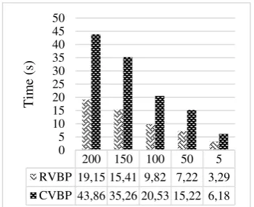
Training time and testing time for RVBP and

CVBP with various hidden neuron and learning

rate can be seen in Figure 7, 8, 9, and 10. From

the experiment result, CVBP performance is

Figure 7. Results of training time in various hidden neuron

Figure 8. Results of training time in various learning rate

200 150 100 50 5 RVBP 19,15 15,41 9,82 7,22 3,29 CVBP 43,86 35,26 20,53 15,22 6,18

0 RVBP 23,05 25,67 24,46 23,29 23,29 CVBP 21,54 20,53 21,19 21,05 20,65

0

Figure 9. Results of testing time in various hidden neuron

Figure 10. Results of testing time in various learning rate

200 150 100 50 5 RVBP 0,04 0,04 0,03 0,04 0,03 CVBP 0,05 0,04 0,04 0,04 0,03

0 RVBP 0,06 0,04 0,04 0,08 0,04 CVBP 0,04 0,04 0,04 0,04 0,04

(7)