VHDL Tutorial
Peter J. Ashenden
EDA C
ONSULTANT, A
SHENDEND
ESIGNSP
TY. L
TD.
www.ashenden.com.au
1
1
Introduction
The purpose of this tutorial is to describe the modeling language VHDL. VHDL in-cludes facilities for describing logical structure and function of digital systems at a number of levels of abstraction, from system level down to the gate level. It is intend-ed, among other things, as a modeling language for specification and simulation. We can also use it for hardware synthesis if we restrict ourselves to a subset that can be automatically translated into hardware.
VHDL arose out of the United States government’s Very High Speed Integrated Circuits (VHSIC) program. In the course of this program, it became clear that there was a need for a standard language for describing the structure and function of inte-grated circuits (ICs). Hence the VHSIC Hardware Description Language (VHDL) was developed. It was subsequently developed further under the auspices of the Institute of Electrical and Electronic Engineers (IEEE) and adopted in the form of the IEEE Stan-dard 1076, Standard VHDL Language Reference Manual, in 1987. This first standard version of the language is often referred to as VHDL-87.
Like all IEEE standards, the VHDL standard is subject to review at least every five years. Comments and suggestions from users of the 1987 standard were analyzed by the IEEE working group responsible for VHDL, and in 1992 a revised version of the standard was proposed. This was eventually adopted in 1993, giving us VHDL-93. A further round of revision of the standard was started in 1998. That process was com-pleted in 2001, giving us the current version of the language, VHDL-2002.
This tutorial describes language features that are common to all versions of the language. They are expressed using the syntax of VHDL-93 and subsequent versions. There are some aspects of syntax that are incompatible with the original VHDL-87 ver-sion. However, most tools now support at least VHDL-93, so syntactic differences should not cause problems.
3
2
Fundamental Concepts
2.1
Modeling Digital Systems
The term digital systems encompasses a range of systems from low-level components to complete system-on-a-chip and board-level designs. If we are to encompass this range of views of digital systems, we must recognize the complexity with which we are dealing. It is not humanly possible to comprehend such complex systems in their entirety. We need to find methods of dealing with the complexity, so that we can, with some degree of confidence, design components and systems that meet their re-quirements.
The most important way of meeting this challenge is to adopt a systematic meth-odology of design. If we start with a requirements document for the system, we can design an abstract structure that meets the requirements. We can then decompose this structure into a collection of components that interact to perform the same func-tion. Each of these components can in turn be decomposed until we get to a level where we have some ready-made, primitive components that perform a required function. The result of this process is a hierarchically composed system, built from the primitive elements.
The advantage of this methodology is that each subsystem can be designed inde-pendently of others. When we use a subsystem, we can think of it as an abstraction rather than having to consider its detailed composition. So at any particular stage in the design process, we only need to pay attention to the small amount of information relevant to the current focus of design. We are saved from being overwhelmed by masses of detail.
We use the term model to mean our understanding of a system. The model rep-resents that information which is relevant and abstracts away from irrelevant detail. The implication of this is that there may be several models of the same system, since different information is relevant in different contexts. One kind of model might con-centrate on representing the function of the system, whereas another kind might rep-resent the way in which the system is composed of subsystems.
There are a number of important motivations for formalizing this idea of a model, including
• expressing system requirements in a complete and unambiguous way
• documenting the functionality of a system
• formally verifying properties of a design
• synthesizing an implementation in a target technology (e.g., ASIC or FPGA)
The unifying factor is that we want to achieve maximum reliability in the design process for minimum cost and design time. We need to ensure that requirements are clearly specified and understood, that subsystems are used correctly and that designs meet the requirements. A major contributor to excessive cost is having to revise a design after manufacture to correct errors. By avoiding errors, and by providing better tools for the design process, costs and delays can be contained.
2.2
VHDL Modeling Concepts
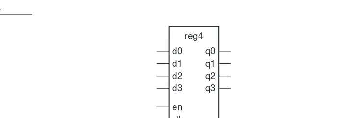
In this section, we look at the basic VHDL concepts for behavioral and structural mod-eling. This will provide a feel for VHDL and a basis from which to work in later chap-ters. As an example, we look at ways of describing a four-bit register, shown in Figure 2-1.
Using VHDL terminology, we call the module reg4 a design entity, and the inputs and outputs are ports. Figure 2-2 shows a VHDL description of the interface to this entity. This is an example of an entity declaration. It introduces a name for the entity and lists the input and output ports, specifying that they carry bit values (‘0’ or ‘1’) into and out of the entity. From this we see that an entity declaration describes the external view of the entity.
FIGURE 2-1
A four-bit register module. The register is named reg4 and has six inputs, d0, d1, d2, d3, en and clk, and four outputs, q0, q1, q2 and q3.
FIGURE 2-2
entity reg4 is
port ( d0, d1, d2, d3, en, clk : in bit;
q0, q1, q2, q3 : out bit ); endentity reg4;
A VHDL entity description of a four-bit register.
reg4
d0 q0
q1 q2 q3 d1 d2 d3
VHDL Modeling Concepts 5
Elements of Behavior
In VHDL, a description of the internal implementation of an entity is called an archi-tecture body of the entity. There may be a number of different architecture bodies of the one interface to an entity, corresponding to alternative implementations that per-form the same function. We can write a behavioral architecture body of an entity, which describes the function in an abstract way. Such an architecture body includes only process statements, which are collections of actions to be executed in sequence. These actions are called sequential statements and are much like the kinds of state-ments we see in a conventional programming language. The types of actions that can be performed include evaluating expressions, assigning values to variables, condition-al execution, repeated execution and subprogram ccondition-alls. In addition, there is a sequen-tial statement that is unique to hardware modeling languages, the signal assignment statement. This is similar to variable assignment, except that it causes the value on a signal to be updated at some future time.
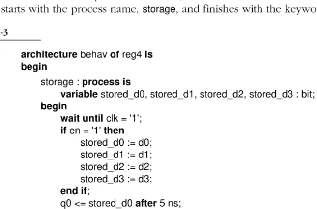
To illustrate these ideas, let us look at a behavioral architecture body for the reg4
entity, shown in Figure 2-3. In this architecture body, the part after the first begin key-word includes one process statement, which describes how the register behaves. It starts with the process name, storage, and finishes with the keywords end process.
FIGURE 2-3
architecture behav of reg4 is begin
storage : processis
variable stored_d0, stored_d1, stored_d2, stored_d3 : bit; begin
wait until clk = '1'; if en = '1' then
stored_d0 := d0; stored_d1 := d1; stored_d2 := d2; stored_d3 := d3;
endif;
q0 <= stored_d0 after 5 ns;
q1 <= stored_d1 after 5 ns;
q2 <= stored_d2 after 5 ns;
q3 <= stored_d3 after 5 ns; endprocess storage;
endarchitecture behav;
A behavioral architecture body of the reg4 entity. The process statement defines a sequence of actions that are to take place when the system is simulated. These actions control how the values on the entity’s ports change over time; that is, they control the behavior of the entity. This process can modify the values of the entity’s ports using signal assignment statements.
after the keyword variable) are initialized to ‘0’, then the statements are executed in order. The first statement is a wait statement that causes the process to suspend. Whil the process is suspended, it is sensitive to the clk signal. When clk changes value to ‘1’, the process resumes.
The next statement is a condition that tests whether the en signal is ‘1’. If it is, the statements between the keywords then and end if are executed, updating the pro-cess’s variables using the values on the input signals. After the conditional if state-ment, there are four signal assignment statements that cause the output signals to be updated 5 ns later.
When the process reaches the end of the list of statements, they are executed again, starting from the keyword begin, and the cycle repeats. Notice that while the process is suspended, the values in the process’s variables are not lost. This is how the process can represent the state of a system.
Elements of Structure
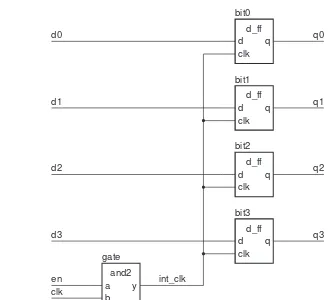
An architecture body that is composed only of interconnected subsystems is called a structural architecture body. Figure 2-4 shows how the reg4 entity might be com-posed of D-flipflops. If we are to describe this in VHDL, we will need entity declara-tions and architecture bodies for the subsystems, shown in Figure 2-5.
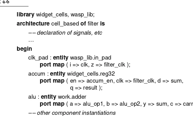
Figure 2-6 is a VHDL architecture body declaration that describes the structure shown in Figure 2-4. The signal declaration, before the keyword begin, defines the internal signals of the architecture. In this example, the signal int_clk is declared to carry a bit value (‘0’ or ‘1’). In general, VHDL signals can be declared to carry arbi-trarily complex values. Within the architecture body the ports of the entity are also treated as signals.
In the second part of the architecture body, a number of component instances are created, representing the subsystems from which the reg4 entity is composed. Each component instance is a copy of the entity representing the subsystem, using the cor-responding basic architecture body. (The name work refers to the current working li-brary, in which all of the entity and architecture body descriptions are assumed to be held.)
The port map specifies the connection of the ports of each component instance to signals within the enclosing architecture body. For example, bit0, an instance of the d_ff entity, has its port d connected to the signal d0, its port clk connected to the signal int_clk and its port q connected to the signal q0.
Test Benches
VHDL Modeling Concepts 7
FIGURE 2-4
A structural composition of the reg4 entity. FIGURE 2-5
entity d_ff is
port ( d, clk : in bit; q : out bit ); end d_ff;
architecture basic of d_ff is begin
ff_behavior : processis begin
wait until clk = '1';
q <= d after 2 ns; endprocess ff_behavior; endarchitecture basic;
––––––––––––––––––––––––––––––––––––––––––––––––––––
entity and2 is
port ( a, b : in bit; y : out bit ); end and2;
architecture basic of and2 is begin
and2_behavior : processis begin
y <= a and b after 2 ns; waiton a, b;
endprocess and2_behavior; endarchitecture basic;
Entity declarations and architecture bodies for D-flipflop and two-input and gate.
FIGURE 2-6
architecture struct of reg4 is signal int_clk : bit; begin
bit0 : entity work.d_ff(basic) portmap (d0, int_clk, q0);
bit1 : entity work.d_ff(basic) portmap (d1, int_clk, q1);
bit2 : entity work.d_ff(basic) portmap (d2, int_clk, q2);
bit3 : entity work.d_ff(basic) portmap (d3, int_clk, q3);
gate : entity work.and2(basic) portmap (en, clk, int_clk); endarchitecture struct;
A VHDL structural architecture body of the reg4 entity. A test bench model for the behavioral implementation of the reg4 register is shown in Figure 2-7. The entity declaration has no port list, since the test bench is entirely self-contained. The architecture body contains signals that are connected to the input and output ports of the component instance dut, the device under test. The process labeled stimulus provides a sequence of test values on the input signals by performing signal assignment statements, interspersed with wait statements. We can use a simulator to observe the values on the signals q0 to q3 to verify that the register operates correctly. When all of the stimulus values have been applied, the stimulus process waits indefinitely, thus completing the simulation.
FIGURE 2-7
entity test_bench is endentity test_bench;
architecture test_reg4 of test_bench is
VHDL Modeling Concepts 9
dut : entity work.reg4(behav)
portmap ( d0, d1, d2, d3, en, clk, q0, q1, q2, q3 );
stimulus : processis begin
d0 <= '1'; d1 <= '1'; d2 <= '1'; d3 <= '1'; en <= '0'; clk <= '0';
wait for 10 ns;
en <= '1'; wait for 10 ns;
clk = '1', '0' after 10 ns; wait for 20 ns;
d0 <= '0'; d1 <= '0'; d2 <= '0'; d3 <= '0'; en <= '0'; wait for 10 ns;
clk <= '1', '0' after 10 ns; wait for 20 ns;
…
wait;
endprocess stimulus; endarchitecture test_reg4;
A VHDL test bench for the reg4 register model.
Analysis, Elaboration and Execution
One of the main reasons for writing a model of a system is to enable us to simulate it. This involves three stages: analysis,elaboration and execution. Analysis and elab-oration are also required in preparation for other uses of the model, such as logic syn-thesis.
In the first stage, analysis, the VHDL description of a system is checked for various kinds of errors. Like most programming languages, VHDL has rigidly defined syntax and semantics. The syntax is the set of grammatical rules that govern how a model is written. The rules of semantics govern the meaning of a program. For example, it makes sense to perform an addition operation on two numbers but not on two pro-cesses.
During the analysis phase, the VHDL description is examined, and syntactic and static semantic errors are located. The whole model of a system need not be analyzed at once. Instead, it is possible to analyze design units, such as entity and architecture body declarations, separately. If the analyzer finds no errors in a design unit, it creates an intermediate representation of the unit and stores it in a library. The exact mech-anism varies between VHDL tools.
The second stage in simulating a model, elaboration, is the act of working through the design hierarchy and creating all of the objects defined in declarations. The ulti-mate product of design elaboration is a collection of signals and processes, with each process possibly containing variables. A model must be reducible to a collection of signals and processes in order to simulate it.
previous value on the signal, an event occurs, and other processes sensitive to the sig-nal may be resumed.
The simulation starts with an initialization phase, followed by repetitive execu-tion of a simulation cycle. During the initialization phase, each signal is given an ini-tial value, depending on its type. The simulation time is set to zero, then each process instance is activated and its sequential statements executed. Usually, a process will include a signal assignment statement to schedule a transaction on a signal at some later simulation time. Execution of a process continues until it reaches a wait state-ment, which causes the process to be suspended.
11
3
VHDL is Like a
Programming Language
3.1
Lexical Elements and Syntax
When we learn a new language, we need to learn how to write the basic elements, such as numbers and identifiers. We also need to learn the syntax, that is, the gram-mar rules governing how we form language constructs. We will briefly describe the lexical elements and our notation for the grammar rules, and then start to introduce langauge features.
VHDL uses characters in the ISO 8859 Latin-1 8-bit character set. This includes uppercase and lowercase letters (including letters with diacritical marks, such as ‘à’, ‘ä’ and so forth), digits 0 to 9, punctuation and other special characters.
Comments
When we are writing a hardware model in VHDL, it is important to annotate the code with comments. A VHDL model consists of a number of lines of text. A comment can be added to a line by writing two dashes together, followed by the comment text. For example:
… a line of VHDL description … –– a descriptive comment
The comment extends from the two dashes to the end of the line and may include any text we wish, since it is not formally part of the VHDL model. The code of a model can include blank lines and lines that only contain comments, starting with two dashes. We can write long comments on successive lines, each starting with two dashes, for example:
–– The following code models –– the control section of the system … some VHDL code …
Identifiers
• may only contain alphabetic letters (‘A’ to ‘Z’ and ‘a’ to ‘z’), decimal digits (‘0’ to ‘9’) and the underline character (‘_’);
• must start with an alphabetic letter;
• may not end with an underline character; and
• may not include two successive underline characters.
Case of letters is not significant. Some examples of valid basic identifiers are
A X0 counter Next_Value generate_read_cycle
Some examples of invalid basic identifiers are
last@value –– contains an illegal character for an identifier
5bit_counter –– starts with a nonalphabetic character
_A0 –– starts with an underline
A0_ –– ends with an underline
clock__pulse –– two successive underlines
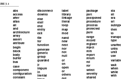
Reserved Words
Some identifiers, called reserved words or keywords, are reserved for special use in VHDL, so we cannot use them as identifiers for items we define. The full list of re-served words is shown in Figure 3-1.
FIGURE 3-1 abs access after alias all and architecture array assert attribute begin block body buffer bus case component configuration constant disconnect downto else elsif end entity exit file for function generate generic group guarded if impure in inertial inout is label library linkage literal loop map mod nand new next nor not null of on open or others out package port postponed procedure process protected pure range record register reject rem report return rol ror select severity shared signal sla sll sra srl subtype then to transport type unaffected units until use variable wait when while with xnor xor
Lexical Elements and Syntax 13
Numbers
There are two forms of numbers that can be written in VHDL code: integer literals and real literals. An integer literal simply represents a whole number and consists of digits without a decimal point. Real literals, on the other hand, can represent fractional numbers. They always include a decimal point, which is preceded by at least one digit and followed by at least one digit. Some examples of decimal integer literals are
23 0 146
Some examples of real literals are
23.1 0.0 3.14159
Both integer and real literals can also use exponential notation, in which the num-ber is followed by the letter ‘E’ or ‘e’, and an exponent value. This indicates a power of 10 by which the number is multiplied. For integer literals, the exponent must not be negative, whereas for real literals, it may be either positive or negative. Some ex-amples of integer literals using exponential notation are
46E5 1E+12 19e00
Some examples of real literals using exponential notation are
1.234E09 98.6E+21 34.0e–08
Characters
A character literal can be written in VHDL code by enclosing it in single quotation marks. Any of the printable characters in the standard character set (including a space character) can be written in this way. Some examples are
'A' –– uppercase letter
'z' –– lowercase letter
',' –– the punctuation character comma
''' –– the punctuation character single quote
' ' –– the separator character space
Strings
A string literal represents a sequence of characters and is written by enclosing the characters in double quotation marks. The string may include any number of charac-ters (including zero), but it must fit entirely on one line. Some examples are
"A string"
"We can include any printing characters (e.g., &%@^*) in a string!!" "00001111ZZZZ"
If we need to include a double quotation mark character in a string, we write two double quotation mark characters together. The pair is interpreted as just one char-acter in the string. For example:
"A string in a string: ""A string"". "
If we need to write a string that is longer than will fit on one line, we can use the concatenation operator (“&”) to join two substrings together. For example:
"If a string will not fit on one line, "
& "then we can break it into parts on separate lines."
Bit Strings
VHDL includes values that represent bits (binary digits), which can be either ‘0’ or ‘1’. A bit-string literal represents a sequence of these bit values. It is represented by a string of digits, enclosed by double quotation marks and preceded by a character that specifies the base of the digits. The base specifier can be one of the following:
• B for binary,
• O for octal (base 8) and
• X for hexadecimal (base 16).
For example, some bitstring literals specified in binary are
B"0100011" B"10" b"1111_0010_0001" B""
Notice that we can include underline characters in bit-string literals to make the literal more readable. The base specifier can be in uppercase or lowercase. The last of the examples above denotes an empty bit string.
If the base specifier is octal, the digits ‘0’ through ‘7’ can be used. Each digit rep-resents exactly three bits in the sequence. Some examples are
O"372" –– equivalent to B"011_111_010"
o"00" –– equivalent to B"000_000"
If the base specifier is hexadecimal, the digits ‘0’ through ‘9’ and ‘A’ through ‘F’ or ‘a’ through ‘f’ (representing 10 through 15) can be used. In hexadecimal, each digit represents exactly four bits. Some examples are
X"FA" –– equivalent to B"1111_1010"
x"0d" –– equivalent to B"0000_1101"
Syntax Descriptions
Lexical Elements and Syntax 15
left of a “⇐” sign (read as “is defined to be”), and a pattern on the right. The simplest kind of pattern is a collection of items in sequence, for example:
variable_assignment ⇐ target := expression ;
This rule indicates that a VHDL clause in the category “variable_assignment” is defined to be a clause in the category “target”, followed by the symbol “:=”, followed by a clause in the category “expression”, followed by the symbol “;”.
The next kind of rule to consider is one that allows for an optional component in a clause. We indicate the optional part by enclosing it between the symbols “[” and “]”. For example:
function_call ⇐ name [ ( association_list ) ]
This indicates that a function call consists of a name that may be followed by an as-sociation list in parentheses. Note the use of the outline symbols for writing the pat-tern in the rule, as opposed to the normal solid symbols that are lexical elements of VHDL.
In many rules, we need to specify that a clause is optional, but if present, it may be repeated as many times as needed. For example, in this rule:
process_statement ⇐ process is
{ process_declarative_item } begin
{ sequential_statement } end process ;
the curly braces specify that a process may include zero or more process declarative items and zero or more sequential statements. A case that arises frequently in the rules of VHDL is a pattern consisting of some category followed by zero or more repetitions of that category. In this case, we use dots within the braces to represent the repeated category, rather than writing it out again in full. For example, the rule
case_statement ⇐ case expression is
case_statement_alternative { … }
end case ;
indicates that a case statement must contain at least one case statement alternative, but may contain an arbitrary number of additional case statement alternatives as re-quired. If there is a sequence of categories and symbols preceding the braces, the dots represent only the last element of the sequence. Thus, in the example above, the dots represent only the case statement alternative, not the sequence “case expres-sion is case_statement_alternative”.
identifier_list ⇐ identifier { , … }
specifies that an identifier list consists of one or more identifiers, and that if there is more than one, they are separated by comma symbols. Note that the dots always rep-resent a repetition of the category immediately preceding the left brace symbol. Thus, in the above rule, it is the identifier that is repeated, not the comma.
Many syntax rules allow a category to be composed of one of a number of alter-natives, specified using the “I” symbol. For example, the rule
mode ⇐ in I out I inout
specifies that the category “mode” can be formed from a clause consisting of one of the reserved words chosen from the alternatives listed.
The final notation we use in our syntax rules is parenthetic grouping, using the symbols “(“ and “)”. These simply serve to group part of a pattern, so that we can avoid any ambiguity that might otherwise arise. For example, the inclusion of paren-theses in the rule
term ⇐ factor { ( * I / I mod I rem ) factor }
makes it clear that a factor may be followed by one of the operator symbols, and then another factor.
This EBNF notation is sufficient to describe the complete grammar of VHDL. However, there are often further constraints on a VHDL description that relate to the meaning of the constructs used. To express such constraints, many rules include ad-ditional information relating to the meaning of a language feature. For example, the rule shown above describing how a function call is formed is augmented thus:
function_call ⇐function_name [ ( parameter_association_list ) ]
The italicized prefix on a syntactic category in the pattern simply provides semantic information. This rule indicates that the name cannot be just any name, but must be the name of a function. Similarly, the association list must describe the parameters supplied to the function.
In this tutorial, we will introduce each new feature of VHDL by describing its syn-tax using EBNF rules, and then we will describe the meaning and use of the feature through examples. In many cases, we will start with a simplified version of the syntax to make the description easier to learn and come back to the full details in a later sec-tion.
3.2
Constants and Variables
Constants and Variables 17
Both constants and variables need to be declared before they can be used in a model. A declaration simply introduces the name of the object, defines its type and may give it an initial value. The syntax rule for a constant declaration is
constant_declaration ⇐
constant identifier { , … } : subtype_indication := expression ;
Here are some examples of constant declarations:
constant number_of_bytes : integer := 4;
constant number_of_bits : integer := 8 * number_of_bytes; constant e : real := 2.718281828;
constant prop_delay : time := 3 ns;
constant size_limit, count_limit : integer := 255;
The form of a variable declaration is similar to a constant declaration. The syntax rule is
variable_declaration ⇐
variable identifier { , … } : subtype_indication [ := expression ] ;
The initialization expression is optional; if we omit it, the default initial value as-sumed by the variable when it is created depends on the type. For scalar types, the default initial value is the leftmost value of the type. For example, for integers it is the smallest representable integer. Some examples of variable declarations are
variable index : integer := 0;
variable sum, average, largest : real; variable start, finish : time := 0 ns;
Constant and variable declarations can appear in a number of places in a VHDL model, including in the declaration parts of processes. In this case, the declared object can be used only within the process. One restriction on where a variable declaration may occur is that it may not be placed so that the variable would be accessible to more than one process. This is to prevent the strange effects that might otherwise occur if the processes were to modify the variable in indeterminate order.
Once a variable has been declared, its value can be modified by an assignment state-ment. The syntax of a variable assignment statement is given by the rule
variable_assignment_statement ⇐ name := expression ;
The name in a variable assignment statement identifies the variable to be changed, and the expression is evaluated to produce the new value. The type of this value must match the type of the variable. Here are some examples of assignment statements:
program_counter := 0; index := index + 1;
3.3
Scalar Types
A scalar type is one whose values are indivisible. In this section, we review VHDL’s predefined scalar types. We will also show how to define new enumeration types.
Subtypes
In many models, we want to declare objects that should only take on a restricted range of values. We do so by first declaring a subtype, which defines a restricted set of val-ues from a base type. The simplified syntax rules for a subtype declaration are
subtype_declaration ⇐ subtype identifier is subtype_indication ;
subtype_indication ⇐
type_mark range simple_expression ( to I downto ) simple_expression
We will look at other forms of subtype indications later. The subtype declaration defines the identifier as a subtype of the base type specified by the type mark, with the range constraint restricting the values for the subtype.
Integer Types
In VHDL, integer types have values that are whole numbers. The predefined type
integer includes all the whole numbers representable on a particular host computer. The language standard requires that the type integer include at least the numbers – 2,147,483,647 to +2,147,483,647 (–231+ 1 to +231– 1), but VHDL implementations may extend the range.
There are also two predefined integer subtypes
natural, containing the integers from 0 to the largest integer, and
positive, containing the integers from 1 to the largest integer.
Where the logic of a design indicates that a number should not be negative, it is good style to use one of these subtypes rather than the base type integer. In this way, we can detect any design errors that incorrectly cause negative numbers to be produced. The operations that can be performed on values of integer types include the fa-miliar arithmetic operations:
+ addition, or unary identity
– subtraction, or unary negation
* multiplication
/ division (with truncation)
mod modulo (same sign as right operand)
rem remainder (same sign as left operand)
abs absolute value
Scalar Types 19
EXAMPLE
Here is a declaration that defines a subtype of integer:
subtype small_int is integer range –128 to 127;
Values of small_int are constrained to be within the range –128 to 127. If we de-clare some variables:
variable deviation : small_int; variable adjustment : integer;
we can use them in calculations:
deviation := deviation + adjustment;
Floating-Point Types
Floating-point types in VHDL are used to represent real numbers with a mantissa part and an exponent part. The predefined floating-point type real includes the greatest range allowed by the host’s floating-point representation. In most implementations, this will be the range of the IEEE 64-bit double-precision representation.
The operations that can be performed on floating-point values include the arith-metic operations addition and unary identity (“+”), subtraction and unary negation (“–
”), multiplication (“*”), division (“/”), absolute value (abs) and exponentiation (“**”). For the binary operators (those that take two operands), the operands must be of the same type. The exception is that the right operand of the exponentiation operator must be an integer.
Time
VHDL has a predefined type called time that is used to represent simulation times and delays. We can write a time value as a numeric literal followed by a time unit. For example:
5 ns 22 us 471.3 msec
Notice that we must include a space before the unit name. The valid unit names are
fs ps ns us ms sec min hr
The type time includes both positive and negative values. VHDL also has a rede-fined subtype of time, delay_length, that only includes non-negative values.
Many of the arithmetic operators can be applied to time values, but with some restrictions. The addition, subtraction, identity and negation operators can be applied to yield results of type time. A time value can be multiplied or divided by an integer
or real value to yield a time value, and two time values can be divided to yield an in-teger. For example:
Finally, the abs operator may be applied to a time value, for example:
abs 2 ps = 2 ps, abs (–2 ps) = 2 ps
Enumeration Types
Often when writing models of hardware at an abstract level, it is useful to use a set of names for the encoded values of some signals, rather than committing to a bit-level encoding straightaway. VHDL enumeration types allow us to do this. In order to de-fine an enumeration type, we need to use a type declaration. The syntax rule is
type_declaration ⇐ type identifier is type_definition ;
A type declaration allows us to introduce a new type, distinct from other types. One form of type definition is an enumeration type definition. We will see other forms later. The syntax rule for enumeration type definitions is
enumeration_type_definition ⇐( ( identifier I character_literal ) { , … } )
This simply lists all of the values in the type. Each value may be either an iden-tifier or a character literal. An example including only ideniden-tifiers is
type alu_function is (disable, pass, add, subtract, multiply, divide);
An example including just character literals is
type octal_digit is ('0', '1', '2', '3', '4', '5', '6', '7');
Given the above two type declarations, we could declare variables:
variable alu_op : alu_function; variable last_digit : octal_digit := '0';
and make assignments to them:
alu_op := subtract; last_digit := '7';
Characters
The predefined enumeration type character includes all of the characters in the ISO 8859 Latin-1 8-bit character set. The type definition is shown in Figure 3-2. It con-taining a mixture of identifiers (for control characters) and character literals (for graph-ic characters). The character at position 160 is a non-breaking space character, distinct from the ordinary space character, and the character at position 173 is a soft hyphen.
FIGURE 3-2
type character is (
nul, soh, stx, etx, eot, enq, ack, bel,
bs, ht, lf, vt, ff, cr, so, si,
Scalar Types 21
can, em, sub, esc, fsp, gsp, rsp, usp,
' ', '!', '"', '#', '$', '%', '&', ''',
'(', ')', '*', '+', ',', '–', '.', '/',
'0', '1', '2', '3', '4', '5', '6', '7',
'8', '9', ':', ';', '<', '=', '>', '?',
'@', 'A', 'B', 'C', 'D', 'E', 'F', 'G',
'H', 'I', 'J', 'K', 'L', 'M', 'N', 'O',
'P', 'Q', 'R', 'S', 'T', 'U', 'V', 'W',
'X', 'Y', 'Z', '[', '\', ']', '^', '_',
'`', 'a', 'b', 'c', 'd', 'e', 'f', 'g',
'h', 'i', 'j', 'k', 'l', 'm', 'n', 'o',
'p', 'q', 'r', 's', 't', 'u', 'v', 'w',
'x', 'y', 'z', '{', '|', '}', '~', del,
c128, c129, c130, c131, c132, c133, c134, c135, c136, c137, c138, c139, c140, c141, c142, c143, c144, c145, c146, c147, c148, c149, c150, c151, c152, c153, c154, c155, c156, c157, c158, c159,
' ', '¡', '¢', '£', '¤', '¥', '¦', '§',
'¨', '©', 'ª', '«', '¬', '-', '®', '¯',
'°', '±', '²', '³', '´', 'µ', '¶', '·',
'¸', '¹', 'º', '»', '¼', '½', '¾', '¿',
'À', 'Á', 'Â', 'Ã', 'Ä', 'Å', 'Æ', 'Ç',
'È', 'É', 'Ê', 'Ë', 'Ì', 'Í', 'Î', 'Ï',
'Ð', 'Ñ', 'Ò', 'Ó', 'Ô', 'Õ', 'Ö', '×',
'Ø', 'Ù', 'Ú', 'Û', 'Ü', 'Ý', 'Þ', 'ß',
'à', 'á', 'â', 'ã', 'ä', 'å', 'æ', 'ç',
'è', 'é', 'ê', 'ë', 'ì', 'í', 'î', 'ï',
'ð', 'ñ', 'ò', 'ó', 'ô', 'õ', 'ö', '÷',
'ø', 'ù', 'ú', 'û', 'ü', 'ý', 'þ', 'ÿ');
The definition of the predefined enumeration type character. To illustrate the use of the character type, we declare variables as follows:
variable cmd_char, terminator : character;
and then make the assignments
cmd_char := 'P'; terminator := cr;
Booleans
The predefined type boolean is defined as
type boolean is (false, true);
relational operators equality (“=”) and inequality (“/=”) can be applied to operands of any type, provided both are of the same type. For example, the expressions
123 = 123, 'A' = 'A', 7 ns = 7 ns
all yield the value true, and the expressions
123 = 456, 'A' = 'z', 7 ns = 2 us
yield the value false.
The relational operators that test ordering are the less-than (“<”), less-than-or-equal-to (“<=”), greater-than (“>”) and greater-than-or-equal-to (“>=”) operators. These can only be applied to values of types that are ordered, including all of the sca-lar types described in this chapter.
The logical operators and, or, nand, nor, xor, xnor and not take operands that must be Boolean values, and they produce Boolean results.
Bits
Since VHDL is used to model digital systems, it is useful to have a data type to repre-sent bit values. The predefined enumeration type bit serves this purpose. It is defined as
type bit is ('0', '1');
The logical operators that we mentioned for Boolean values can also be applied to values of type bit, and they produce results of type bit. The value ‘0’ corresponds to false, and ‘1’ corresponds to true. So, for example:
'0' and '1' = '0', '1' xor '1' = '0'
The difference between the types boolean and bit is that boolean values are used to model abstract conditions, whereas bit values are used to model hardware logic levels. Thus, ‘0’ represents a low logic level and ‘1’ represents a high logic level.
Standard Logic
The IEEE has standardized a package called std_logic_1164 that allows us to model digital signals taking into account some electrical effects. One of the types defined in this package is an enumeration type called std_ulogic, defined as
type std_ulogic is ( 'U', –– Uninitialized
'X', –– Forcing Unknown
'0', –– Forcing zero
'1', –– Forcing one
'Z', –– High Impedance
'W', –– Weak Unknown
'L', –– Weak zero
'H', –– Weak one
Sequential Statements 23
This type can be used to represent signals driven by active drivers (forcing strength), resistive drivers such as pull-ups and pull-downs (weak strength) or three-state drivers including a high-impedance three-state. Each kind of driver may drive a “zero”, “one” or “unknown” value. An “unknown” value is driven by a model when it is un-able to determine whether the signal should be “zero” or “one”. In addition to these values, the leftmost value in the type represents an “uninitialized” value. If we declare signals of std_ulogic type, by default they take on ‘U’ as their initial value. The final value in std_ulogic is a “don’t care” value. This is sometimes used by logic synthesis tools and may also be used when defining test vectors, to denote that the value of a signal to be compared with a test vector is not important.
Even though the type std_ulogic and the other types defined in the std_logic_1164
package are not actually built into the VHDL language, we can write models as though they were, with a little bit of preparation. For now, we describe some “magic” to include at the beginning of a model that uses the package; we explain the details later. If we include the line
library ieee; use ieee.std_logic_1164.all;
preceding each entity or architecture body that uses the package, we can write models as though the types were built into the language.
With this preparation in hand, we can now create constants, variables and signals of type std_ulogic. As well as assigning values of the type, we can also use the logical operators and, or, not and so on. Each of these operates on std_ulogic values and returns a std_ulogic result of ‘U’, ‘X’, ‘0’ or ‘1’.
3.4
Sequential Statements
In this section we look at how data may be manipulated within processes using se-quential statements, so called because they are executed in sequence. We have al-ready seen one of the basic sequential statements, the variable assignment statement. The statements we look at in this section deal with controlling actions within a model; hence they are often called control structures. They allow selection between alterna-tive courses of action as well as repetition of actions.
If Statements
In many models, the behavior depends on a set of conditions that may or may not hold true during the course of simulation. We can use an if statement to express this behavior. The syntax rule for an if statement is
if_statement ⇐ [ if_label : ]
if boolean_expression then { sequential_statement } { elsif boolean_expression then
{ sequential_statement } ] end if [ if_label ] ;
A simple example of an if statement is
if en = '1' then
stored_value := data_in;
endif;
The Boolean expression after the keyword if is the condition that is used to con-trol whether or not the statement after the keyword then is executed. If the condition evaluates to true, the statement is executed. We can also specify actions to be per-formed if the condition is false. For example:
if sel = 0 then
result <= input_0; –– executed if sel = 0 else
result <= input_1; –– executed if sel /= 0 endif;
Here, as the comments indicate, the first signal assignment statement is executed if the condition is true, and the second signal assignment statement is executed if the condition is false.
We can construct a more elaborate form of if statement to to check a number of different conditions, for example:
if mode = immediate then
operand := immed_operand;
elsif opcode = load or opcode = add or opcode = subtract then
operand := memory_operand;
else
operand := address_operand;
endif;
In general, we can construct an if statement with any number of elsif clauses (in-cluding none), and we may include or omit the else clause. Execution of the if state-ment starts by evaluating the first condition. If it is false, successive conditions are evaluated, in order, until one is found to be true, in which case the corresponding statements are executed. If none of the conditions is true, and we have included an else clause, the statements after the else keyword are executed.
EXAMPLE
Sequential Statements 25
Figure 3-3 shows the entity and architecture bodies for the thermostat. The entity declaration defines the input and output ports. The process in the archi-tecture body includes the input ports in the sensitivity list after the keyword proc-ess. This is a list of signals to which the process is sensitive. When any of these signals changes value, the process resumes and executes the sequential state-ments. After it has executed the last statement, the process suspends again. The if statement compares the actual temperature with the desired temperature and turns the heater on or off as required.
FIGURE 3-3
entity thermostat is
port ( desired_temp, actual_temp : in integer;
heater_on : out boolean ); endentity thermostat;
––––––––––––––––––––––––––––––––––––––––––––––––––––
architecture example of thermostat is begin
controller : process (desired_temp, actual_temp) is begin
if actual_temp < desired_temp – 2 then
heater_on <= true;
elsif actual_temp > desired_temp + 2 then
heater_on <= false;
endif;
endprocess controller; endarchitecture example;
An entity and architecture body for a heater thermostat.
Case Statements
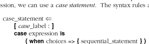
If we have a model in which the behavior is to depend on the value of a single ex-pression, we can use a case statement. The syntax rules are as follows:
case_statement ⇐ [ case_label : ] case expression is
( when choices => { sequential_statement } ) { … }
end case [ case_label ] ;
choices ⇐ ( simple_expression I discrete_range I others ) { | … }
For example, suppose we are modeling an arithmetic/logic unit, with a control input, func, declared to be of the enumeration type:
We could describe the behavior using a case statement:
case func is when pass1 =>
result := operand1;
when pass2 =>
result := operand2;
when add =>
result := operand1 + operand2;
when subtract =>
result := operand1 – operand2;
endcase;
At the head of this case statement is the selector expression, between the keywords case and is. The value of this expression is used to select which statements to exe-cute. The body of the case statement consists of a series of alternatives. Each alter-native starts with the keyword when and is followed by one or more choices and a sequence of statements. The choices are values that are compared with the value of the selector expression. There must be exactly one choice for each possible value. The case statement finds the alternative whose choice value is equal to the value of the selector expression and executes the statements in that alternative.
We can include more than one choice in each alternative by writing the choices separated by the “|” symbol. For example, if the type opcodes is declared as
type opcodes is
(nop, add, subtract, load, store, jump, jumpsub, branch, halt);
we could write an alternative including three of these values as choices:
when load | add | subtract =>
operand := memory_operand;
If we have a number of alternatives in a case statement and we want to include an alternative to handle all possible values of the selector expression not mentioned in previous alternatives, we can use the special choice others. For example, if the variable opcode is a variable of type opcodes, declared above, we can write
case opcode is
when load | add | subtract =>
operand := memory_operand;
when store | jump | jumpsub | branch =>
operand := address_operand;
whenothers =>
operand := 0;
endcase;
Sequential Statements 27
An important point to note about the choices in a case statement is that they must all be written using locally static values. This means that the values of the choices must be determined during the analysis phase of design processing.
EXAMPLE
We can write a behavioral model of a branch-condition multiplexer with a select input sel; two condition code inputs cc_z and cc_c; and an output taken. The condition code inputs and outputs are of the IEEE standard-logic type, and the select input is of type branch_fn, which we assume to be declared elsewhere as
type branch_fn is (br_z, br_nz, br_c, br_nc);
We will see later how we define a type for use in an entity declaration. The entity declaration defining the ports and a behavioral architecture body are shown in Figure 3-4. The architecture body contains a process that is sensitive to the inputs. It makes use of a case statement to select the value to assign to the output.
FIGURE 3-4
library ieee; use ieee.std_logic_1164.all; entity cond_mux is
port ( sel : in barnch_fn;
cc_z, cc_c : in std_ulogic;
taken : out std_ulogic ); endentity cond_mux;
––––––––––––––––––––––––––––––––––––––––––––––––––––
architecture demo of cond_mux is begin
out_select : process (sel, cc_z, cc_c) is begin
case sel is when br_z =>
taken <= cc_z;
when br_nz =>
taken <= not cc_z; when br_c =>
taken <= cc_c;
when br_nc =>
taken <= not cc_c; endcase;
endprocess out_select; endarchitecture demo;
Loop and Exit Statements
Often we need to write a sequence of statements that is to be repeatedly executed. We use a loop statement to express this behavior. The syntax rule for a simple loop that iterates indefinitely is
loop_statement ⇐ [ loop_label : ] loop
{ sequential_statement } end loop [ loop_label ] ;
Usually we need to exit the loop when some condition arises. We can use an exit statement to exit a loop. The syntax rule is
exit_statement ⇐
[ label : ] exit [ loop_label ] [ when boolean_expression ] ;
The simplest form of exit statement is just
exit;
When this statement is executed, any remaining statements in the loop are skipped, and control is transferred to the statement after the end loop keywords. So in a loop we can write
ifconditionthen exit;
endif;
where condition is a Boolean expression. Since this is perhaps the most common use of the exit statement, VHDL provides a shorthand way of writing it, using the when clause. We use an exit statement with the when clause in a loop of the form
loop
…
exitwhencondition; …
endloop;
… –– control transferred to here
–– when condition becomes true within the loop
EXAMPLE
Sequential Statements 29
FIGURE 3-5
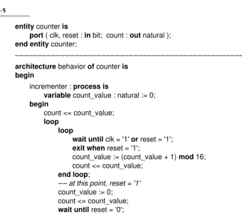
entity counter is
port ( clk, reset : in bit; count : out natural ); endentity counter;
––––––––––––––––––––––––––––––––––––––––––––––––––––
architecture behavior of counter is begin
incrementer : processis
variable count_value : natural := 0; begin
count <= count_value;
loop loop
waituntil clk = '1' or reset = '1'; exitwhen reset = '1';
count_value := (count_value + 1) mod 16;
count <= count_value;
endloop;
–– at this point, reset = '1'
count_value := 0; count <= count_value;
waituntil reset = '0'; endloop;
endprocess incrementer; endarchitecture behavior;
An entity and architecture body of the revised counter, including a reset input. The architecture body contains two nested loops. The inner loop deals with normal counting operation. When reset changes to ‘1’, the exit statement causes the inner loop to be terminated. Control is transferred to the statement just after the end of the inner loop. The count value and count outputs are reset, and the process then waits for reset to return to ‘0’, after which the process resumes and the outer loop repeats.
In some cases, we may wish to transfer control out of an inner loop and also a containing loop. We can do this by labeling the outer loop and using the label in the exit statement. We can write
loop_name : loop
…
exit loop_name;
…
This labels the loop with the name loop_name, so that we can indicate which loop to exit in the exit statement. The loop label can be any valid identifier. The exit state-ment referring to this label can be located within nested loop statestate-ments.
While Loops
We can augment the basic loop statement introduced previously to form a while loop, which tests a condition before each iteration. If the condition is true, iteration pro-ceeds. If it is false, the loop is terminated. The syntax rule for a while loop is
loop_statement ⇐ [ loop_label : ]
while boolean_expression loop { sequential_statement } end loop [ loop_label ] ;
The only difference between this form and the basic loop statement is that we have added the keyword while and the condition before the loop keyword. All of the things we said about the basic loop statement also apply to a while loop. The con-dition is tested before each iteration of the while loop, including the first iteration. This means that if the condition is false before we start the loop, it is terminated im-mediately, with no iterations being executed.
EXAMPLE
We can develop a model for an entity cos that calculates the cosine function of an input theta using the relation
We add successive terms of the series until the terms become smaller than one millionth of the result. The entity and architecture body declarations are shown in Figure 3-6. The cosine function is computed using a while loop that incre-ments n by two and uses it to calculate the next term based on the previous term. Iteration proceeds as long as the last term computed is larger in magnitude than one millionth of the sum. When the last term falls below this threshold, the while loop is terminated.
FIGURE 3-6
entity cos is
port ( theta : in real; result : out real ); endentity cos;
––––––––––––––––––––––––––––––––––––––––––––––––––––
architecture series of cos is begin
θ
cos 1 θ
2
2!
---– θ
4
4! --- θ
6
6!
---– …
+ +
Sequential Statements 31
summation : process (theta) is variable sum, term : real; variable n : natural; begin
sum := 1.0; term := 1.0; n := 0;
whileabs term > abs (sum / 1.0E6) loop
n := n + 2;
term := (–term) * theta**2 / real(((n–1) * n)); sum := sum + term;
endloop;
result <= sum;
endprocess summation; endarchitecture series;
An entity and architecture body for a cosine module.
For Loops
Another way we can augment the basic loop statement is the for loop. A for loop includes a specification of how many times the body of the loop is to be executed. The syntax rule for a for loop is
loop_statement ⇐ [ loop_label : ]
for identifier in discrete_range loop { sequential_statement } end loop [ loop_label ] ;
A discrete range can be of the form
simple_expression ( to I downto ) simple_expression
representing all the values between the left and right bounds, inclusive. The identifier is called the loop parameter, and for each iteration of the loop, it takes on successive values of the discrete range, starting from the left element. For example, in this for loop:
for count_value in 0 to 127 loop
count_out <= count_value;
waitfor 5 ns; endloop;
the identifier count_value takes on the values 0, 1, 2 and so on, and for each value, the assignment and wait statements are executed. Thus the signal count_out will be assigned values 0, 1, 2 and so on, up to 127, at 5 ns intervals.
cannot make assignments to it. Unlike other constants, we do not need to declare it. Instead, the loop parameter is implicitly declared over the for loop. It only exists when the loop is executing, and not before or after it.
Like basic loop statements, for loops can enclose arbitrary sequential statements, including exit statements, and we can label a for loop by writing the label before the for keyword.
EXAMPLE
We now rewrite the cosine model in Figure 3-6 to calculate the result by sum-ming the first 10 terms of the series with a for loop. The entity declaration is un-changed. The revised architecture body is shown in Figure 3-7.
FIGURE 3-7
architecture fixed_length_series of cos is begin
summation : process (theta) is variable sum, term : real; begin
sum := 1.0; term := 1.0;
for n in 1 to 9 loop
term := (–term) * theta**2 / real(((2*n–1) * 2*n)); sum := sum + term;
endloop;
result <= sum;
endprocess summation; endarchitecture fixed_length_series;
The revised architecture body for the cosine module.
Assertion Statements
One of the reasons for writing models of computer systems is to verify that a design functions correctly. We can partially test a model by applying sample inputs and checking that the outputs meet our expectations. If they do not, we are then faced with the task of determining what went wrong inside the design. This task can be made easier using assertion statements that check that expected conditions are met within the model. An assertion statement is a sequential statement, so it can be in-cluded anywhere in a process body. The syntax rule for an assertion statement is
assertion_statement ⇐
assert boolean_expression
[ report expression ] [ severity expression ] ;
state-Sequential Statements 33
ment is executed. If the condition is not met, we say that an assertion violation has occurred. If an assertion violation arises during simulation of a model, the simulator reports the fact. For example, if we write
assert initial_value <= max_value;
and initial_value is larger than max_value when the statement is executed during sim-ulation, the simulator will let us know.
We can get the simulator to provide extra information by including a report clause in an assertion statement, for example:
assert initial_value <= max_value report "initial value too large";
The string that we provide is used to form part of the assertion violation message. VHDL predefines an enumeration type severity_level, defined as
type severity_level is (note, warning, error, failure);
We can include a value of this type in a severity clause of an assertion statement. This value indicates the degree to which the violation of the assertion affects operation of the model. Some example are:
assert packet_length /= 0
report "empty network packet received" severity warning;
assert clock_pulse_width >= min_clock_width severity error;
If we omit the report clause, the default string in the error message is “Assertion violation.” If we omit the severity clause, the default value is error. The severity value is usually used by a simulator to determine whether or not to continue execution after an assertion violation. Most simulators allow the user to specify a severity threshold, beyond which execution is stopped.
EXAMPLE
An important use for assertion statements is in checking timing constraints that apply to a model. For example, in an edge-triggered register, when the clock changes from ‘0’ to ‘1’, the data input is sampled, stored and transmitted through to the output. Let us suppose that the clock input must remain at ‘1’ for at least 5 ns. Figure 3-8 is a model for a register that includes a check for legal clock pulse width.
FIGURE 3-8
entity edge_triggered_register is port ( clock : in bit;
––––––––––––––––––––––––––––––––––––––––––––––––––––
architecture check_timing of edge_triggered_register is begin
store_and_check : process (clock) is variable stored_value : real; variable pulse_start : time; begin
case clock is when '1' =>
pulse_start := now; stored_value := d_in; d_out <= stored_value;
when '0' =>
assert now = 0 ns or (now – pulse_start) >= 5 ns report "clock pulse too short";
endcase;
endprocess store_and_check; endarchitecture check_timing;
An entity and architecture body for an edge-triggered register, including a timing check for correct pulse width on the clock input.
The architecture body contains a process that is sensitive to changes on the clock input. When the clock changes from ‘0’ to ‘1’, the input is stored, and the current simulation time, accessed using the predefined function now, is recorded in the variable pulse_start. When the clock changes from ‘1’ to ‘0’, the difference between pulse_start and the current simulation time is checked by the assertion statement.
3.5
Array Types and Operations
An array consists of a collection of values, all of which are of the same type as each other. The position of each element in an array is given by a scalar value called its index. To create an array object in a model, we first define an array type in a type declaration. The syntax rule for an array type definition is
array_type_definition ⇐
array ( discrete_range ) of element_subtype_indication
This defines an array type by specifying the index range and the element type or sub-type. A discrete range is a subset of values from a discrete type (an integer or enu-meration type). It can be specified as shown by the simplified syntax rule
discrete_range ⇐ type_mark
Array Types and Operations 35
We illustrate these rules for defining arrays with a series of examples. Here is a simple example to start off with, showing the declaration of an array type to represent words of data:
type word isarray (0 to 31) of bit;
Each element is a bit, and the elements are indexed from 0 up to 31. An alterna-tive declaration of a word type, more appropriate for “little-endian” systems, is
type word isarray (31 downto 0) of bit;
The difference here is that index values start at 31 for the leftmost element in val-ues of this type and continue down to 0 for the rightmost. The index valval-ues of an array do not have to be numeric. For example, given this declaration of an enumer-ation type:
type controller_state is (initial, idle, active, error);
we could then declare an array as follows:
type state_counts isarray (idle to error) of natural;
If we need an array element for every value in an index type, we need only name the index type in the array declaration without specifying the range. For example:
subtype coeff_ram_address is integer range 0 to 63; type coeff_array isarray (coeff_ram_address) of real;
Once we have declared an array type, we can define objects of that type, includ-ing constants, variables and signals. For example, usinclud-ing the types declared above, we can declare variables as follows:
variable buffer_register, data_register : word; variable counters : state_counts;
variable coeff : coeff_array;
Each of these objects consists of the collection of elements described by the corre-sponding type declaration. An individual element can be used in an expression or as the target of an assignment by referring to the array object and supplying an index value, for example:
coeff(0) := 0.0;
If active is a variable of type controller_state, we can write
counters(active) := counters(active) + 1;
An array object can also be used as a single composite object. For example, the assignment
copies all of the elements of the array buffer_register into the corresponding elements of the array data_register.
Array Aggregates
Often we also need to write literal array values, for example, to initialize a variable or constant of an array type. We can do this using a VHDL construct called an array aggregate, according to the syntax rule
aggregate ⇐( ( [ choices => ] expression ) { , … } )
Let us look first at the form of aggregate without the choices part. It simply con-sists of a list of the elements enclosed in parentheses, for example:
type point isarray (1 to 3) of real; constant origin : point := (0.0, 0.0, 0.0); variable view_point : point := (10.0, 20.0, 0.0);
This form of array aggregate uses positional association to determine which value in the list corresponds to which element of the array. The first value is the element with the leftmost index, the second is the next index to the right, and so on, up to the last value, which is the element with the rightmost index. There must be a one-to-one correspondence between values in the aggregate and elements in the array.
An alternative form of aggregate uses named association, in which the index val-ue for each element is written explicitly using the choices part shown in the syntax rule. The choices may be specified in exactly the same way as those in alternatives of a case statement. For example, the variable declaration and initialization could be rewritten as
variable view_point : point := (1 => 10.0, 2 => 20.0, 3 => 0.0);
EXAMPLE
Figure 3-9 is a model for a memory that stores 64 real-number coefficients, initialized to 0.0. We assume the type coeff_ram_address is previously declared as above. The architecture body contains a process with an array variable repre-senting the coefficient storage. The array is initialized using an aggregate in which all elements are 0.0. The process is sensitive to all of the input ports. When
rd is ‘1’, the array is indexed using the address value to read a coefficient. When
wr is ‘1’, the address value is used to select which coefficient to change.
FIGURE 3-9
entity coeff_ram is
port ( rd, wr : in bit; addr : in coeff_ram_address;
d_in : in real; d_out : out real ); endentity coeff_ram;
––––––––––––––––––––––––––––––––––––––––––––––––––––
Array Types and Operations 37
memory : process (rd, wr, addr, d_in) is
type coeff_array isarray (coeff_ram_address) of real; variable coeff : coeff_array := (others => 0.0); begin
if rd = '1' then
d_out <= coeff(addr);
endif; if wr = '1' then
coeff(addr) := d_in;
endif; endprocess memory; endarchitecture abstract;
An entity and architecture body for a memory module that stores real-number coefficients. The mem-ory storage is implemented using an array.
Array Attributes
VHDL provides a number of attributes to refer to information about the index ranges of array types and objects. Attributes are written by following the array type or object name with the symbol ' and the attribute name. Given some array type or object A, and an integer N between 1 and the number of dimensions of A, VHDL defines the following attributes:
A'left Left bound of index range of A A'right Right bound of index range of A A'range Index range of A
A'reverse_range Reverse of index range of A A'length Length of index range of A
For example, given the array declaration
type A isarray (1 to 4) of boolean;
some attribute values are
A'left = 1 A'right = 4
A'range is 1 to 4 A'reverse_range is 4 downto 1
A'length = 4
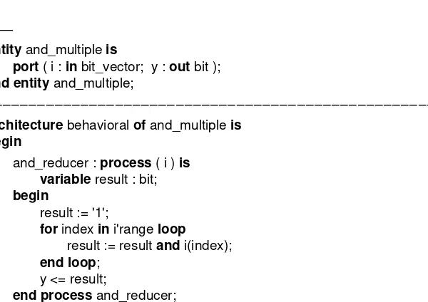
The attributes can be used when writing for loops to iterate over elements of an array. For example, given an array variable free_map that is an array of bits, we can write a for loop to count the number of ‘1’ bits without knowing the actual size of the array:
count := 0;
count := count + 1;
endif; endloop;
The 'range and 'reverse_range attributes can be used in any place in a VHDL model where a range specification is required, as an alternative to specifying the left and right bounds and the range direction. Thus, we may use the attributes in type and subtype definitions, in subtype constraints, in for loop parameter specifications, in case state-ment choices and so on. The advantage of taking this approach is that we can specify the size of the array in one place in the model and in all other places use array at-tributes. If we need to change the array size later for some reason, we need only change t