Jan Camenisch (Eds.)
123
LNCS 10719
24th International Conference
Ottawa, ON, Canada, August 16–18, 2017
Revised Selected Papers
Selected Areas
Commenced Publication in 1973 Founding and Former Series Editors:
Gerhard Goos, Juris Hartmanis, and Jan van Leeuwen
Editorial Board
David HutchisonLancaster University, Lancaster, UK Takeo Kanade
Carnegie Mellon University, Pittsburgh, PA, USA Josef Kittler
University of Surrey, Guildford, UK Jon M. Kleinberg
Cornell University, Ithaca, NY, USA Friedemann Mattern
ETH Zurich, Zurich, Switzerland John C. Mitchell
Stanford University, Stanford, CA, USA Moni Naor
Weizmann Institute of Science, Rehovot, Israel C. Pandu Rangan
Indian Institute of Technology, Madras, India Bernhard Steffen
TU Dortmund University, Dortmund, Germany Demetri Terzopoulos
University of California, Los Angeles, CA, USA Doug Tygar
University of California, Berkeley, CA, USA Gerhard Weikum
Selected Areas
in Cryptography
–
SAC 2017
24th International Conference
Ottawa, ON, Canada, August 16
–
18, 2017
Revised Selected Papers
School of Electrical Engineering and Computer Science (SITE) University of Ottawa
Ottawa, ON Canada
IBM Research - Zurich Rueschlikon
Switzerland
ISSN 0302-9743 ISSN 1611-3349 (electronic) Lecture Notes in Computer Science
ISBN 978-3-319-72564-2 ISBN 978-3-319-72565-9 (eBook) https://doi.org/10.1007/978-3-319-72565-9
Library of Congress Control Number: 2017962894 LNCS Sublibrary: SL4–Security and Cryptology ©Springer International Publishing AG 2018
This work is subject to copyright. All rights are reserved by the Publisher, whether the whole or part of the material is concerned, specifically the rights of translation, reprinting, reuse of illustrations, recitation, broadcasting, reproduction on microfilms or in any other physical way, and transmission or information storage and retrieval, electronic adaptation, computer software, or by similar or dissimilar methodology now known or hereafter developed.
The use of general descriptive names, registered names, trademarks, service marks, etc. in this publication does not imply, even in the absence of a specific statement, that such names are exempt from the relevant protective laws and regulations and therefore free for general use.
The publisher, the authors and the editors are safe to assume that the advice and information in this book are believed to be true and accurate at the date of publication. Neither the publisher nor the authors or the editors give a warranty, express or implied, with respect to the material contained herein or for any errors or omissions that may have been made. The publisher remains neutral with regard to jurisdictional claims in published maps and institutional affiliations.
Printed on acid-free paper
This Springer imprint is published by Springer Nature The registered company is Springer International Publishing AG
The Conference on Selected Areas in Cryptography (SAC) is the leading Canadian venue for the presentation and publication of cryptographic research. The 24th annual SAC was held this year at the University of Ottawa, Ontario (for the second time; the first was in 2007). In keeping with its tradition, SAC 2017 offered a relaxed and collegial atmosphere for researchers to present and discuss new results.
SAC has three regular themes:
– Design and analysis of symmetric key primitives and cryptosystems, including block and stream ciphers, hash functions, MAC algorithms, and authenticated encryption schemes
– Efficient implementations of symmetric and public key algorithms – Mathematical and algorithmic aspects of applied cryptology
The following special (or focus) theme for this year was: – Post-quantum cryptography
A total of 66 submissions were received, out of which the Program Committee selected 23 papers for presentation. It is our pleasure to thank the authors of all the submissions for the high quality of their work. The review process was thorough (each submission received the attention of at least three reviewers, and at least five for submissions involving a Program Committee member).
There were two invited talks. The Stafford Tavares Lecture was given by Helena Handschuh, who presented “Test Vector Leakage Assessment Methodology: An Update,” and the second invited talk was given by Chris Peikert, who presented “Lattice Cryptography: From Theory to Practice, and Back Again.”
This year, SAC hosted what is now the third iteration of the SAC Summer School (S3). S3 is intended to be a place where young researchers can increase their knowl-edge of cryptography through instruction by, and interaction with, leading researchers. This year, we were fortunate to have Michele Mosca, Douglas Stebila, and David Jao presenting post-quantum cryptographic algorithms, Tanja Lange and Daniel J. Bern-stein presenting public key cryptographic algorithms, and Orr Dunkelman presenting symmetric key cryptographic algorithms. We would like to express our sincere grati-tude to these six presenters for dedicating their time and effort to what has become a highly anticipated and highly beneficial event for all participants.
Finally, the members of the Program Committee, especially the co-chairs, would like to thank the additional reviewers, who gave generously of their time to assist with the paper review process. We are also very grateful to our sponsors, Microsoft and Communications Security Establishment, whose enthusiastic support (both financial and otherwise) greatly contributed to the success of SAC this year.
October 2017 Jan Camenisch
The 24th Annual Conference on Selected Areas in Cryptography Ottawa, Ontario, Canada, August 16–18, 2017
Program Chairs
Carlisle Adams University of Ottawa, Canada Jan Camenisch IBM Research - Zurich, Switzerland
Program Committee
Carlisle Adams (Co-chair) University of Ottawa, Canada Shashank Agraval Visa Research, USA
Elena Andreeva COSIC, KU Leuven, Belgium
Kazumaro Aoki NTT, Japan
Jean-Philippe Aumasson Kudelski Security, Switzerland
Roberto Avanzi ARM, Germany
Manuel Barbosa HASLab - INESC TEC and FCUP, Portugal Paulo Barreto University of São Paulo, Brazil
Andrey Bogdanov Technical University of Denmark, Denmark Billy Brumley Tampere University of Technology, Finland Jan Camenisch (Co-chair) IBM Research - Zurich, Switzerland Itai Dinur Ben-Gurion University, Israel Maria Dubovitskaya IBM Research - Zurich, Switzerland Guang Gong University of Waterloo, Canada
Johann Groszschaedl University of Luxembourg, Luxembourg Tim Güneysu University of Bremen and DFKI, Germany M. Anwar Hasan University of Waterloo, Canada
Howard Heys Memorial University, Canada
Laurent Imbert CNRS, LIRMM, UniversitéMontpellier 2, France Michael Jacobson University of Calgary, Canada
Elif Bilge Kavun Infineon Technologies AG, Germany
Stephan Krenn Austrian Institute of Technology GmbH, Austria Juliane Krämer Technische Universität Darmstadt, Germany Thijs Laarhoven IBM Research - Zurich, Switzerland Gaëtan Leurent Inria, France
Petr Lisonek Simon Fraser University, Canada María Naya-Plasencia Inria, France
Francesco Regazzoni ALaRI - USI, Switzerland Palash Sarkar Indian Statistical Institute, India
Kyoji Shibutani Sony Corporation, Japan
Francesco Sica Nazarbayev University, Kazakhstan Daniel Slamanig Graz University of Technology, Austria
Meltem Sonmez Turan National Institute of Standards and Technology, USA Michael Tunstall Cryptography Research, USA
Discrete Logarithms
Second Order Statistical Behavior of LLL and BKZ . . . 3 Yang Yu and Léo Ducas
Refinement of the Four-Dimensional GLV Method on Elliptic Curves . . . 23 Hairong Yi, Yuqing Zhu, and Dongdai Lin
Key Agreement
Post-Quantum Static-Static Key Agreement Using Multiple
Protocol Instances . . . 45 Reza Azarderakhsh, David Jao, and Christopher Leonardi
Side-Channel Attacks on Quantum-Resistant Supersingular
Isogeny Diffie-Hellman . . . 64 Brian Koziel, Reza Azarderakhsh, and David Jao
Theory
Computing Discrete Logarithms inFp6 . . . 85 Laurent Grémy, Aurore Guillevic,
François Morain, and Emmanuel Thomé
Computing Low-Weight Discrete Logarithms . . . 106 Bailey Kacsmar, Sarah Plosker, and Ryan Henry
Efficient Implementation
sLiSCP: Simeck-Based Permutations for Lightweight Sponge
Cryptographic Primitives . . . 129 Riham AlTawy, Raghvendra Rohit, Morgan He,
Kalikinkar Mandal, Gangqiang Yang, and Guang Gong Efficient Reductions in Cyclotomic Rings - Application
to Ring-LWE Based FHE Schemes . . . 151 Jean-Claude Bajard, Julien Eynard, Anwar Hasan,
How to (Pre-)Compute a Ladder: Improving the Performance
of X25519 and X448. . . 172 Thomaz Oliveira, Julio López, Hüseyin Hışıl, Armando Faz-Hernández,
and Francisco Rodríguez-Henríquez
HILA5: On Reliability, Reconciliation, and Error Correction
for Ring-LWE Encryption . . . 192 Markku-Juhani O. Saarinen
Public Key Encryption
A Public-Key Encryption Scheme Based on Non-linear
Indeterminate Equations . . . 215 Koichiro Akiyama, Yasuhiro Goto, Shinya Okumura,
Tsuyoshi Takagi, Koji Nuida, and Goichiro Hanaoka
NTRU Prime: Reducing Attack Surface at Low Cost . . . 235 Daniel J. Bernstein, Chitchanok Chuengsatiansup,
Tanja Lange, and Christine van Vredendaal
Signatures
Leighton-Micali Hash-Based Signatures in the Quantum
Random-Oracle Model. . . 263 Edward Eaton
Efficient Post-Quantum Undeniable Signature on 64-Bit ARM . . . 281 Amir Jalali, Reza Azarderakhsh, and Mehran Mozaffari-Kermani
“Oops, I Did It Again”– Security of One-Time Signatures
Under Two-Message Attacks . . . 299 Leon Groot Bruinderink and Andreas Hülsing
Cryptanalysis
Low-Communication Parallel Quantum Multi-Target Preimage Search . . . 325 Gustavo Banegas and Daniel J. Bernstein
Lattice Klepto: Turning Post-Quantum Crypto Against Itself . . . 336 Robin Kwant, Tanja Lange, and Kimberley Thissen
Total Break of the SRP Encryption Scheme . . . 355 Ray Perlner, Albrecht Petzoldt, and Daniel Smith-Tone
Approximate Short Vectors in Ideal Lattices ofQðfpeÞ
Quantum Key-Recovery on Full AEZ . . . 394 Xavier Bonnetain
Quantum Key Search with Side Channel Advice. . . 407 Daniel P. Martin, Ashley Montanaro, Elisabeth Oswald,
and Dan Shepherd
Multidimensional Zero-Correlation Linear Cryptanalysis
of Reduced Round SPARX-128 . . . 423 Mohamed Tolba, Ahmed Abdelkhalek, and Amr M. Youssef
Categorising and Comparing Cluster-Based DPA Distinguishers . . . 442 Xinping Zhou, Carolyn Whitnall, Elisabeth Oswald, Degang Sun,
and Zhu Wang
of LLL and BKZ
Yang Yu1(B) and L´eo Ducas2(B)
1 Department of Computer Science and Technology, Tsinghua University, Beijing, China
2 Cryptology Group, CWI, Amsterdam, The Netherlands [email protected]
Abstract. The LLL algorithm (from Lenstra, Lenstra and Lov´asz) and its generalization BKZ (from Schnorr and Euchner) are widely used in cryptanalysis, especially for lattice-based cryptography. Precisely under-standing their behavior is crucial for deriving appropriate key-size for cryptographic schemes subject to lattice-reduction attacks. Current mod-els, e.g. the Geometric Series Assumption and Chen-Nguyen’s BKZ-simulator, have provided a decent first-order analysis of the behavior of LLL and BKZ. However, they only focused on theaveragebehavior and were not perfectly accurate. In this work, we initiate asecond order analy-sisof this behavior. We confirm and quantify discrepancies between mod-els and experiments —in particular in the head and tail regions— and study their consequences. We also provide variationsaround the mean and correlations statistics, and study their impact. While mostly based on experiments, by pointing at and quantifyingunaccounted phenomena, our study sets the ground for a theoretical and predictive understanding of LLL and BKZ performances at the second order.
Keywords: Lattice reduction
·
LLL·
BKZ·
Cryptanalysis·
Statistics1
Introduction
Lattice reduction is a powerful algorithmic tool for solving a wide range of prob-lems ranging from integer optimization probprob-lems and probprob-lems from algebra or number theory. Lattice reduction has played a role in the cryptanalysis of cryptosystems not directly related to lattices, and is now even more relevant to quantifying the security of lattice-based cryptosystems [1,6,14].
The goal of lattice reduction is to find a basis with short and nearly orthog-onal vectors. In 1982, the first polynomial time lattice reduction algorithm, LLL [15], was invented by Lenstra, Lenstra and Lov´asz. Then, the idea of block-wise reduction appeared and several block-wise lattice reduction algo-rithms [7,8,19,24] were proposed successively. Currently, BKZ is the most prac-tical lattice reduction algorithm. Schnorr and Euchner first put forward the orig-inal BKZ algorithm in [24]. It is subject to many heuristic optimizations, such as early-abort [12], pruned enumeration [10] and progressive reduction [2,4].
c
Springer International Publishing AG 2018
All such improvements have been combined in the so-called BKZ 2.0 algorithm of Chen and Nguyen [5] (progressive strategy was improved further in later work [2]). Also, plenty of analyses [2,9,19,23,31] of BKZ algorithms have been made to explore and predict the performance of BKZ algorithms, which provide rough security estimations for lattice-based cryptography.
Despite of their popularity, the behavior of lattice reduction algorithms is still not completely understood. While there are reasonable models (e.g. the Geometric Series Assumption [25] and simulators [5]), there are few studies on the experimental statistical behavior of those algorithms, and they considered rather outdated versions of those algorithms [3,20,23]. The accuracy of the cur-rent model remains unclear.
This state of affair is quite problematic to evaluate accurately the concrete security level of lattice-based cryptosystem proposal. With the recent calls for post-quantum schemes by the NIST, this matter seems pressing.
Our Contribution.In this work, we partially address this matter, by proposing a second-order statistical (for random input bases) analysis of the behavior of reduction algorithms in practice, qualitatively and quantitatively. We figure out one more low order term in the predicted average value of several quantities such as the root Hermite factor. Also, we investigate the variation around the average behavior, a legitimate concern raised by Micciancio and Walter [19].
In more details, we experimentally study the logarithms of ratios between two adjacent Gram-Schmidt norms in LLL and BKZ-reduced basis (denotedri’s below). We highlight three ranges for the statistical behavior of theri: the head (i≤h), the body (h < i < n−t) and the tail (i ≥n−t). The lengths of the head and tail are essentially determined by the blocksizeβ. In the body range, the statistical behavior of the ri’s are similar: this does not only provide new support for the so-called Geometric Series Assumption [25] when β ≪ n, but also a refinement of it applicable even when β≪n. We note in particular that the impact of the head on the root Hermite factor is much stronger than the impact of the tail.
We also study the variance and the covariance between theri’s. We observe a local correlation between theri’s. More precisely we observe thatri andri+1are negatively correlated, inducing a self-stabilizing behavior of those algorithms: the overall variance is less than the sum of local variances.
Then, we measure the half-volume, i.e.⌊n2⌋
i=1b∗i, a quantity determining the cost of enumeration on reduced basis. By expressing the half-volume using the statistics of the ri’s, we determine that the complexity of enumeration on BKZ-reduced basis should be of the form 2an2
±bn1.5
: the variation around average (denoted by ±) can impact the speed of enumeration by a super-exponential factor.
phenomenon qualitatively and quantitatively, but the head phenomenon is not captured. Thus it is necessary to revise the security estimation and refine the simulator.
Impact. Our work points at several inaccuracies of the current models for the behavior of LLL and BKZ, and quantifies them experimentally. It should be noted that our measured statistics are barely enough to address the question of precise prediction. Many tweaks on those algorithms are typically applied (more aggressive pruning, more subtle progressive reductions, ...) to accelerate them and that would impact those statistics. On the other hand, the optimal parametrization of heuristic tweaks is very painful to reproduce, and not even clearly determined in the literature. We therefore find it preferable to first app-roach stable versions of those algorithm, and minimize the space of parameters. We would also not dare to simply guess extrapolation models for those statis-tics to larger blocksize: this should be the topic of a more theoretical study.
Yet, by pointing out precisely the problematic phenomena, we set the ground for revised models and simulators: our reported statistics can be used to sanity check such future models and simulators.
Source code. Our experiments heavily rely on the latest improvements of the open-source libraryfplll[27], catching up with the state of the art algorithm BKZ 2.0. For convenience, we used the python wrapperfpylll[28] forfplll, making our scripts reasonably concise and readable. All our scripts are open-source and available online2, for reviewing, reproduction or extension purposes.
2
Preliminaries
We refer to [21] for a detailed introduction to lattice reduction and to [12,16] for an introduction to the behavior of LLL and BKZ.
2.1 Notations and Basic Definitions
All vectors are denoted by bold lower case letters and are to be read as row-vectors. Matrices are denoted by bold capital letters. We write a matrix Binto B= (b1,· · · ,bn) wherebiis thei-th row vector ofB. IfB∈Rn×mhas full rank n, the lattice Lgenerated by the basisBis denoted byL(B) ={xB|x∈Zn}. We denote by (b∗
1,· · ·,b∗n) the Gram-Schmidt orthogonalization of the matrix (b1,· · ·,bn). Fori∈ {1,· · ·, n}, we define the orthogonal projection to the span of (b1,· · · ,bi−1)⊥ as π
i. For 1≤i < j≤n, we denote byB[i,j] the local block (πi(bi),· · · , πi(bj)), byL[i,j] the lattice generated by B[i,j].
The Euclidean norm of a vector v is denoted by v. The volume of a lat-tice L(B) is vol(L(B)) =
ib∗i, that is an invariant of the lattice. The first minimum of a lattice L is the length of a shortest non-zero vector, denoted by λ1(L). We use the shorthands vol(B) = vol(L(B)) andλ1(B) =λ1(L(B)).
Given a random variable X, we denote by E(X) its expectation and by Var(X) its variance. Also we denote byCov(X, Y) the covariance between two random variablesXandY. LetX= (X1,· · · , Xn) be a vector formed by random variables, its covariance matrix is defined byCov(X) = (Cov(Xi, Xj))i,j.
2.2 Lattice Reduction: In Theory and in Practice
We now recall the definitions of LLL and BKZ reduction. A basis B is LLL-reduced with parameterδ∈(12,1], if:
1. |µi,j| ≤ 12, 1 ≤ j < i ≤ n, where µi,j = bi,b∗j /b∗j,b∗j are the Gram-Schmidt orthogonalization coefficients;
2. δb∗
i ≤ b∗i+1+µi+1,ib∗i, for 1≤i < n.
A basisBis BKZ-reduced with parameterβ≥2 andδ∈(1 2,1], if: 1. |µi,j| ≤ 12, 1≤j < i≤n;
2. δb∗
i ≤λ1(L[i,min(i+β−1,n)]), for 1≤i < n.
Note that we follow the definition of BKZ reduction from [24] which is a little different from the first notion proposed by Schnorr [26]. We also recall that, as proven in [24], LLL is equivalent to BKZ2. Typically, LLL and BKZ are used withLov´asz parameterδ=√0.99 and so will we.
For high dimensional lattices, running BKZ with a large blocksize is very expensive. Heuristics improvements were developed, and combined by Chen and Nguyen [5], advertised as BKZ 2.0.3 In this paper, we report on pure BKZ
behavior to avoid perturbations due to heuristic whenever possible. Yet we switch to BKZ 2.0 to reach larger blocksizes when deemed relevant.
The two main improvements in BKZ 2.0 are calledearly-abort and pruned enumeration. As proven in [12], the output basis of BKZ algorithm with blocksize β would be of an enough good quality afterC·nβ22
logn+ log log max b∗i vol(L)1/n
tours, whereCis a small constant. In our experiments of BKZ 2.0, we chose dif-ferent C and observed its effect on the final basis. We also applied the pruning heuristic (see [4,10,27] for details) to speed-up enumeration, but chose a con-servative success probability (95%) without re-randomization to avoid altering the quality of the output. The preprocessing-pruning strategies were optimized using the strategizer [29] of fplll/fpylll.
Given a basisBof ann-dimensional latticeL, we denote byrhf(B) the root Hermite factor of B, defined by rhf(B) = b1
vol(L)1/n 1/n
. The root Hermite factor is a common measurement of the reducedness of a basis, e.g. [9].
Let us define the sequence{ri(B)}1≤i≤n−1of ann-dimensional lattice basis B= (b1,· · ·,bn) such thatri(B) = lnb∗i/b∗i+1
. The root Hermite factor rhf(B) can be expressed in terms of theri(B)’s:
rhf(B) = exp ⎛
⎝ 1 n2
1≤i≤n−1
(n−i)ri(B) ⎞
⎠. (1)
Intuitively, the sequence{ri(B)}1≤i≤n−1characterizes how fast the sequence {b∗
i}decreases. Thus Eq. (1) provides an implication between the fact that the b∗
i’s don’t decrease too fast and the fact that the root Hermite factor is small. For reduced bases, theri(B)’s are of certain theoretical upper bounds. However, it is well known that experimentally, the ri(B)’s tend to be much smaller than the theoretical bounds in practice.
From a practical perspective, we are more interested in the behavior of the ri(B)’s for random lattices. The standard notion of random real lattices of given volume is based on Haar measures of classical groups. As shown in [11], the uni-form distribution over integer lattices of volumeV converges to the distribution of random lattices of unit volume, asV grows to infinity. In our experiments, we followed the sampling procedure of the lattice challenges [22]: its volume is a ran-dom prime of bit-length 10nand its Hermite normal form (see [18] for details) is sampled uniformly once its volume is determined. Also, we define a random LLL (resp. BKZβ)-reduced basis as the basis outputted by LLL (resp. BKZβ) applied to a random lattice given by its Hermite normal form, as described above. To speed up convergence, following a simplified progressive strategy [2,4], we run BKZ (resp. BKZ 2.0) with blocksize β = 2,4,6, ... (resp. β = 2,6,10, ...) pro-gressively from the Hermite normal form of a lattice.
We treat theri(B)’s as random variables (under the randomness of the lattice basis before reduction). For any i ∈ {1,· · · , n−1}, we denote by ri(β, n) the random variableri(β, n) =ri(B), whereBis a random BKZβ-reduced basis, and by Di(β, n) the distribution of ri(β, n). When β and nare clear from context, we simply writeri forri(β, n).
2.3 Heuristics on Lattice Reduction
Gaussian Heuristic. The Gaussian Heuristic, denoted by GAUSS, says that, for “any reasonable” subsetKof the span of the latticeL, the number of lattice points insideKis approximately vol(K)/vol(L). Let the volume ofn-dimensional unit ball beVn(1) = π
n/2
Γ(n/2+1). A prediction derived from GAUSS is thatλ1(L)≈ vol(L)1/n·GH(n) where GH(n) = Vn(1)−1/n, which is accurate for random lattices. As suggested in [10,13], GAUSS is a valuable heuristic to estimate the cost and quality of various lattice algorithms.
Random Local Block.In [5], Chen and Nguyen suggested the following mod-eling assumption, seemingly accurate for large enough blocksizes:
By RANDn,β and GAUSS, one can predict the root Hermite factor of local blocks: rhf(B[i,i+β−1])≈GH(β)
1
β.
Geometric Series Assumption.In [25], Schnorr first proposed the Geometric Series Assumption, denoted by GSA, which says that, in typical reduced basisB, the sequence{b∗
i}1≤i≤n looks like a geometric series (while GAUSS provides the exact value of this geometric ratio). GSA provides a simple description of Gram-Schmidt norms and then leads to some estimations of Hermite factor and enumeration complexity [9,10]. When it comes to{ri(B)}1≤i≤n−1, GSA implies that theri(B)’s are supposed to be almost equal to each others. However, GSA is not so perfect, because the first and lastb∗
i’s usually violate it [3]. The behavior in the tail is well explained, and can be predicted and simulated [5].
3
Head and Tail
In [3,5], it was already claimed that for a BKZβ-reduced basis B, GSA doesn’t hold in the first and last indices. We call this phenomenon “Head and Tail”, and provide detailed experiments. Our experiments confirm that GSA holds in a strong sense in the body of the basis (i.e. outside of the head and tail regions). Precisely, the distributions ofri’s are similar in that region, not only their averages. We also confirm the violations of GSA in the head and the tail, quantify them, and exhibit that they are independent of the dimensionn.
As a conclusion, we shall see that the head and tail have only small impacts on the root Hermite factor whenn≫β, but also that they can also be quantitatively handled whenn≫β. We notice that the head has in fact a stronger impact than the tail, which emphasizes the importance of finding models or simulators that capture this phenomenon, unlike the current ones that only capture the tail [5].
3.1 Experiments
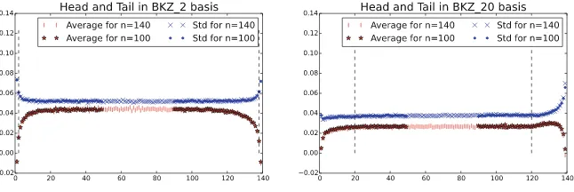
We ran BKZ on many random input lattices and report on the distribution of eachri. We first plot the average and the variance of ri for various blocksizesβ and dimensionsnin Fig.1. By superposing with proper alignment curves for the sameβ but variousn, we notice that the head and tail behavior doesn’t depend on the dimension n, but only on the relative indexi (resp. n−i) in the head (resp. the tail). A more formal statement will be provided in Claim1.
Fig. 1. Average value and standard deviation ofri as a function of i. Experimental values measure over 5000 samples of randomn-dimensional BKZ bases forn= 100,140. First halves {ri}i≤(n−1)/2 are left-aligned while last halves {ri}i>(n−1)/2 are right-aligned so to highlight heads and tails. Dashed lines mark indicesβ andn−β. Plots look similar in blocksizeβ= 6,10,20,30 and in dimensionn= 80,100,120,140, which are provided in the full version.
KS Test on Di(2,100)’s
10 20 30 40 50 60 70 80 90 10
20 30 40 50 60 70 80 90
KS Test on Di(20,100)’s
10 20 30 40 50 60 70 80 90 10
20 30 40 50 60 70 80 90
Fig. 2.Kolmogorov-Smirnov Test with significance level 0.05 on allDi(β,100)’s calcu-lated from 5000 samples of random 100-dimensional BKZ bases with blocksizeβ= 2,20 respectively. A black pixel at position (i, j) marks the fact that the pair of distributions Di(β,100) andDj(β,100) passed Kolmogorov-Smirnov Test,i.e. two distributions are close. Plots in β = 10,30 look similar to that inβ = 20, which are provided in the full version.
3.2 Conclusion
From the experiments above, we allow ourselves to the following conclusion. Experimental Claim 1. There exist two functionsh, t:N→N, such that, for all n, β∈N, and whenn≥h(β) +t(β) + 2:
would not hold when the early-abort strategy is applied. More precisely, the head and tail phenomenon is getting stronger as we apply more tours (see Fig.4).
From now on, we may omit the indexiwhen speaking of the distribution of ri, implicitly implying that the only indices considered are such thath(β)< i < n−t(β). The random variablerdepends on blocksizeβ only, hence we introduce two functions ofβ, e(β) and v(β), to denote the expectation and variance ofr respectively. Also, we denote by ri(h)(resp. rn(t−)i) the ri inside the head (resp.
We conclude by a statement on the impacts of the head and tail on the logarithmic average root Hermite factor:
Corollary 1. For a fixed blocksize β, and as the dimension n grows, it holds that
Corollary 1 indicates that the impacts on the average root Hermite factor from the head and tail are decreasing. In particular, the tail has a very little effect O 1
n2
on the average root Hermite factor. The impact of the headd(β)/n, which hasn’t been quantified in earlier work, is —perhaps surprisingly— asymptotically larger. We include the proof of Corollary1in AppendixA.
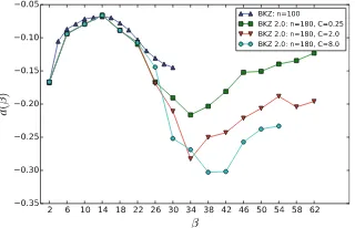
Below, Figs.3 and 4 provide experimental measure of e(β) and d(β) from 5000 random 100-dimensional BKZβ-reduced bases. We note that the lengths of the head and tail seem about the maximum of 15 and β. Thus we seth(β) = t(β) = max(15, β) simply, which affects the measure ofe(β) andd(β) little. For the averagee(2)≈0.043 we recover the experimental root Hermite factor of LLL rhf(B) = exp(0.043/2)≈1.022, compatible with many other experiments [9].
To extend the curves, we also plot the experimental measure ofe(β) andd(β)4 from 20 random 180-dimensional BKZβ 2.0 bases with bounded tour number
. It shows that the qualitative behavior of BKZ 2.0 is different from full-BKZ not only the quantitative one: there is a bump5 in the curve of e(β) when β ∈ [22,30]. Considering that the success
probability for the SVP enumeration was set to 95%, the only viable explanation for this phenomenon in our BKZ 2.0 experiments is the early-abort strategy: the shape of the basis is not so close to the fix-point.
4 For BKZ 2.0, the distributions of ther
i’s inside the body may not be identical, thus we just calculate the mean of thoseri’s as a measure ofe(β).
5 Yet the quality of the basis does not decrease withβ in this range, as the bump on
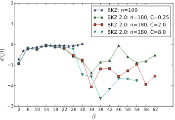
Fig. 3.Experimental measure ofe(β) Fig. 4.Experimental measure ofd(β)
4
Local Correlations and Global Variance
In the previous section, we have classified theri’s and established a connection between the average of the root Hermite factor and the functione(β). Now we are to report on the (co-)variance of the ri’s. Figure5 shows the experimental measure of local variances,i.e.variances of theri’s inside the body, but it is not enough to deduce the global variance,i.e.the variance of the root Hermite factor. We still need to understand more statistics, namely the covariances among these ri’s. Our experiments indicate that local correlations—i.e. correlations between ri andri+1—are negative and other correlations seem to be zero. Moreover, we confirm the tempting hypothesis that local correlations inside the body are all equal and independent of the dimensionn.
Based on these observations, we then express the variance of the logarithm of root Hermite factor for fixedβ and increasingnasymptotically, and quantify the self-stability of LLL and BKZ algorithms.
4.1 Experiments
Let r= (r1,· · ·, rn−1) be the random vector formed by random variables ri’s. We profile the covariance matricesCov(r) for 100-dimensional lattices with BKZ reduction of different blocksizes in Fig.6. The diagonal elements in covariance matrix correspond to the variances of the ri’s which we have studied before. Thus we set all diagonal elements to 0 to enhance contrast. We discover that the elements on the second diagonals, i.e. Cov(ri, ri+1)’s, are significantly nega-tive and other elements seems very close to 0. We call the Cov(ri, ri+1)’s local covariances.
Fig. 6.Covariance matrices of r. Experimental values measure over 5000 samples of random 100-dimensional BKZ bases with blocksizeβ= 2,20. The pixel at coordinates (i, j) corresponds to the covariance betweenriandrj. Plots inβ= 10,30 look similar to that inβ= 20, which are provided in the full version.
We then plot measured local covariances in Fig.7. Comparing these curves for various dimensionsn, we notice that the head and tail parts almost coincide, and the local covariances inside the body seem to depend on β only, we will denote this value by c(β). We also plot the curves of the Cov(ri, ri+2)’s in Fig.7 and note that the curves for theCov(ri, ri+2)’s are horizontal with a value about 0. For otherCov(ri, ri+d)’s with largerd, the curves virtually overlap that for the Cov(ri, ri+2)’s. For readability, larger values ofdare not plotted. One thing to be noted is that the case for blocksizeβ = 2 is an exception. On one hand, the head and tail of the local covariances in BKZ2 basis bend in the opposite directions, unlike for larger β. In particular, the Cov(ri, ri+2)’s in BKZ2 basis are not so close to 0, but are nevertheless significantly smaller than the local covariances Cov(ri, ri+1). That indicates some differences between LLL and BKZ.
Fig. 7. Cov(ri, ri+1) and Cov(ri, ri+2) as a function ofi. Experimental values mea-sured over 5000 samples of random n-dimensional BKZ bases for n = 100,140. The blue curves denote the Cov(ri, ri+1)’s and the red curves denote theCov(ri, ri+2)’s. For same dimension n, the markers in two curves are identical. First halves are left aligned while last halves {Cov(ri, ri+1)}i>(n−2)/2 and {Cov(ri, ri+2)}i>(n−3)/2 are right aligned so to highlight heads and tails. Dashed lines mark indicesβandn−β−2. Plots look similar in blocksizeβ= 6,10,20,30 and in dimension n= 80,100,120,140, which are provided in the full version.
Remark 2. To obtain a precise measure of covariances, we need enough samples and thus the extended experimental measure ofc(β) is not given. Nevertheless, it seems that, after certain number of tours, local covariances of BKZ 2.0 bases still tend to be negative but other covariances tend to zero.
Fig. 8. Experimental measure of the evolution of c(β) calculated from 5000 samples of random BKZ bases in dif-ferent dimensionnrespectively.
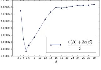
Fig. 9. Experimental measure of v(β)+2c(β)
3 . The data point for β = 2, v(2)+2c(2)
3 ≈ 0.00045 was clipped out, being 10 times larger than all other values.
4.2 Conclusion
1. When|i−j|>1,ri andrj are not correlated: Cov(ri, rj) = 0
One direct consequence derives from the above experimental claim is that the global variance, i.e. the variance of the logarithm of root Hermite factor, converges to 0 asΘ(1/n), where the hidden constant is determined byβ: Corollary 2. For a fixed blocksize β, and as the dimension n grows, it holds that
The proof of Corollary2 is given in AppendixB. Note that the assumption that all Cov(ri, ri+d)’s withd > 1 equal 0 may not be exactly true. However, random BKZ-reduced basisB. As claimed in [10], the nodes in the enumeration tree at the depths around n2 contribute the most to the total node number, for both full and regular pruned enumerations. Typically, the enumeration radiusR is set toc√n·vol(B)1nfor some constantc >0,e.g. R= 1.05·GH(n)·vol(B)
1
n, the number of nodes in the ⌊n
2⌋level is approximately proportional to
H(B) vol(B)⌈n2⌉/n, making the half-volume a good estimator for the cost of enumeration. Those formulas have to be amended in case pruning is used (see [10]), but the half-volume remains a good indicator of the cost of enumeration.
Lethv(β, n) be the random variable ln(H(B))−⌊n2⌋
Corollary 3 (Under previous experimental claims). For a fixed blocksize Assuming heuristically that the variation around the average ofhvfollows a Normal law, Corollary3implies that the complexity of enumeration on a random n-dimensional BKZβ-reduced basis should be of the shape
exp
n2x(β) +y(β)±n1.5l·z(β)
(6) except a fraction at most exp(−l2/2) of random bases, where
x(β) = e(β)
and where the term ±n1.5l·z(β) accounts for variation around the average behavior. In particular, the contribution of the variation around the average remains asymptotically negligible compared to the main exp(Θ(n2)) factor, it still introduces a super-exponential factor, that can make one particular attempt much cheaper or much more expensive in practice. It means that it could be beneficial in practice to rely partially on luck, restarting BKZ without trying enumeration when the basis is unsatisfactory.
The experimental measure of 8x(β) and 16z(β)2 has been shown in Figs.3 and 9 respectively. We now exhibit the experimental measure of y(β) in Fig.10. Despite the curves for BKZ 2.0 are not smooth, it seems that y(β)(=d′(β)) would increase with β when β is large. However, comparing to n2x(β), the impact ofy(β) on the half-volume is still much weaker.6
6
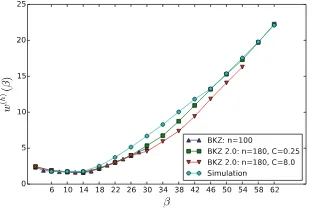
Performance of Simulator
In [5], Chen and Nguyen proposed a simulator to predict the behavior of BKZ. For largeβ, the simulator can provide a reasonable prediction of average profile, i.e. log b∗i
vol(L)1/n
n
i=1. In this section, we will further report on the perfor-mance of the simulator qualitatively and quantitatively. Our experiments confirm that the tail still exists in the simulated result and fits the actual measure, but the head phenomenon is not captured by the simulator, affecting its accuracy for cryptanalytic prediction.
6 The impacts of ther
Fig. 10.Experimental measure ofy(β)(=d′(β))
To make the simulator7coincide with the actual algorithm, we set the param-eterδ=√0.99 and applied a similar progressive strategy8. The maximum tour
number corresponds to the case thatC= 0.25 in [12], but the simulator always terminates after a much smaller number of tours.
6.1 Experiments
We ran simulator on several sequences of different dimensions and plot the aver-age values ofri’s in Fig.11. An apparent tail remains in the simulated result and the length of its most significant part is aboutβ despite a slim stretch. However, there is no distinct head, which does not coincide with the actual behavior: the head shape appears after a few tours of BKZ or BKZ 2.0. Still, the ri’s inside the body share similar values, in accordance with GSA and experiments.
Fig. 11.Average value ofricalculated by simulator. First halves are left aligned while last halves{ri}i>(n−1)/2are right aligned so to highlight heads and tails. The vertical dashed line marks the indexn−βand the horizontal dashed line is used for contrast.
7 We worked on an open-source BKZ simulator [30], with minor modifications. 8 In simulation, the initial profile sequence is set to (10(n−1),−10,· · ·,−10) and
We now compare the average experimental behavior with the simulated result. Note that the simulator is not fed with any randomness, so it does not make sense to consider variance in this comparison.
Figure12illustrates the comparison one(β). For small blocksizeβ, the sim-ulator does not work well, but, as β increases, the simulated measure of e(β) seems close to the experimental measure and both measures converge to the prediction lnGH(β)β−21
.
Fig. 12.Comparison one(β) Fig. 13.Comparison ons(h)(β)
Finally, we consider the two functions d(β) and d′(β) that are relevant to the averages of the logarithms of the root Hermite factor and the complexity of enumeration and defined in Corollarys 1and3respectively. To better under-stand the difference, we compared the following terms s(h)(β) =
i≤he (h) i (β), w(h)(β) =
i≤h i 2e
(h)
i (β) and w(t)(β) =
i≤t i 2e
(t)
i respectively, where we set h(β) = t(β) = max(15, β) as before. Indeed, combined with e(β), these three terms determine d(β) andd′(β).
From Fig.13, we observe that the simulated measure of s(h)(β) is greater than the experimental measure, which is caused by the lack of the head. The similar inaccuracy exists as well with respect tow(h)(β) as shown in Fig.14. The experimental measure ofe(β) is slightly greater than the simulated measure and
thus the e(ih)(β)’s of greater weight may compensate somewhat the lack of the head. After enough tours, the head phenomenon is highlighted and yet the body shape almost remains the same so that the simulator still cannot predictw(h)(β) precisely. Figure15 indicates that the simulator could predict w(t)(β) precisely for both large and small blocksizes and therefore the HKZ-shaped tail model is reasonable.
6.2 Conclusion
Chen and Nguyen’s simulator gives an elementary profile for random BKZβ -reduced bases with large β: both body and tail shapes are reflected well in the simulation result qualitatively and quantitatively. However, the head phe-nomenon is not captured by this simulator, and thus the first b∗
i’s are not predicted accurately. In particular, the prediction ofb∗1 that determines the Hermite factor is usually larger than the actual value, which leads to an underes-timation of the quality of BKZ bases. Consequently, related security esunderes-timations need to be refined.
Understanding the main cause of the head phenomenon, modeling it and refining the simulator to include it seems an interesting and important problem, which we leave to the future work. It would also be interesting to introduce some randomness in the simulator, so to properly predict variance around the mean behavior.
Acknowledgements. We thank Phong Q. Nguyen, Jean-Christophe Deneuville and Guillaume Bonnoron for helpful discussions and comments. We also thank the SAC’17 reviewers for their useful comments. Yang Yu is supported by China’s 973 Program (No. 2013CB834205), the Strategic Priority Research Program of the Chinese Academy of Sciences (No. XDB01010600) and NSF of China (No. 61502269). L´eo Ducas is sup-ported by a Veni Innovational Research Grant from NWO under project number 639.021.645. Parts of this work were done during Yang Yu’s internship at CWI.
and
2 e(β) areO(1). A straightforward computation then leads to the con-clusion.
B
Proof of Corollary
2
We compare the variances of two sides in Eq. (8), then:
n4Var(ln(rhf(B))) = also constant. Thus the two first sums areO(n2). Also, the differencen−1
C
Proof of Corollary
3
Letn′=⌊n
2⌋. A routine computation leads to that:
hv(β, n) =
We compare the expectations of two sides in Eq. (15), then:
E(hv(β, n)) =
Since h and t are constant, the two sums i≤hie We compare the variances of two sides in Eq. (15), then:
Var(hv(β, n)) = Exploiting the identity that n
References
1. Alkim, E., Ducas, L., P¨oppelmann, T., Schwabe, P.: Post-quantum key exchange— a new hope. In: USENIX Security 2016, 327–343 (2016)
2. Aono, Y., Wang, Y., Hayashi, T., Takagi, T.: Improved progressive BKZ algorithms and their precise cost estimation by sharp simulator. In: Fischlin, M., Coron, J.-S. (eds.) EUROCRYPT 2016, Part I. LNCS, vol. 9665, pp. 789–819. Springer, Hei-delberg (2016).https://doi.org/10.1007/978-3-662-49890-3 30
3. Buchmann, J., Ludwig, C.: Practical lattice basis sampling reduction. In: Hess, F., Pauli, S., Pohst, M. (eds.) ANTS 2006. LNCS, vol. 4076, pp. 222–237. Springer, Heidelberg (2006).https://doi.org/10.1007/11792086 17
4. Chen, Y.: R´eduction de r´eseau et s´ecurit´e concr`ete du chiffrement compl`etement homomorphe. PhD thesis (2013)
5. Chen, Y., Nguyen, P.Q.: BKZ 2.0: better lattice security estimates. In: Lee, D.H., Wang, X. (eds.) ASIACRYPT 2011. LNCS, vol. 7073, pp. 1–20. Springer, Heidelberg (2011).https://doi.org/10.1007/978-3-642-25385-0 1
6. Ducas, L., Durmus, A., Lepoint, T., Lyubashevsky, V.: Lattice signatures and bimodal gaussians. In: Canetti, R., Garay, J.A. (eds.) CRYPTO 2013, Part I. LNCS, vol. 8042, pp. 40–56. Springer, Heidelberg (2013).https://doi.org/10.1007/ 978-3-642-40041-4 3
7. Gama, N., Howgrave-Graham, N., Koy, H., Nguyen, P.Q.: Rankin’s constant and blockwise lattice reduction. In: Dwork, C. (ed.) CRYPTO 2006. LNCS, vol. 4117, pp. 112–130. Springer, Heidelberg (2006).https://doi.org/10.1007/11818175 7 8. Gama, N., Nguyen, P.Q.: Finding short lattice vectors within mordell’s inequality.
In: STOC 2008, pp. 207–216 (2008)
9. Gama, N., Nguyen, P.Q.: Predicting lattice reduction. In: Smart, N. (ed.) EURO-CRYPT 2008. LNCS, vol. 4965, pp. 31–51. Springer, Heidelberg (2008).https:// doi.org/10.1007/978-3-540-78967-3 3
10. Gama, N., Nguyen, P.Q., Regev, O.: Lattice enumeration using extreme pruning. In: Gilbert, H. (ed.) EUROCRYPT 2010. LNCS, vol. 6110, pp. 257–278. Springer, Heidelberg (2010).https://doi.org/10.1007/978-3-642-13190-5 13
11. Goldstein, D., Mayer, A.: On the equidistribution of hecke points. Forum Mathe-maticum15(2), 165–189 (2003)
12. Hanrot, G., Pujol, X., Stehl´e, D.: Analyzing blockwise lattice algorithms using dynamical systems. In: Rogaway, P. (ed.) CRYPTO 2011. LNCS, vol. 6841, pp. 447–464. Springer, Heidelberg (2011). https://doi.org/10.1007/978-3-642-22792-9 25
13. Hanrot, G., Stehl´e, D.: Improved analysis of kannan’s shortest lattice vector algo-rithm. In: Menezes, A. (ed.) CRYPTO 2007. LNCS, vol. 4622, pp. 170–186. Springer, Heidelberg (2007).https://doi.org/10.1007/978-3-540-74143-5 10 14. Hoffstein, J., Pipher, J., Silverman, J.H.: NTRU: a ring-based public key
cryptosys-tem. In: Buhler, J.P. (ed.) ANTS 1998. LNCS, vol. 1423, pp. 267–288. Springer, Heidelberg (1998).https://doi.org/10.1007/BFb0054868
15. Lenstra, A.K., Lenstra, H.W., Lov´asz, L.: Factoring polynomials with rational coefficients. Math. Ann.261(4), 515–534 (1982)
16. Madritsch, M., Vall´ee, B.: Modelling the LLL algorithm by sandpiles. In: L´opez-Ortiz, A. (ed.) LATIN 2010. LNCS, vol. 6034, pp. 267–281. Springer, Hei-delberg (2010).https://doi.org/10.1007/978-3-642-12200-2 25
18. Micciancio, D.: Improving lattice based cryptosystems using the hermite normal form. In: Silverman, J.H. (ed.) CaLC 2001. LNCS, vol. 2146, pp. 126–145. Springer, Heidelberg (2001).https://doi.org/10.1007/3-540-44670-2 11
19. Micciancio, D., Walter, M.: Practical, predictable lattice basis reduction. In: Fischlin, M., Coron, J.-S. (eds.) EUROCRYPT 2016, Part I. LNCS, vol. 9665, pp. 820–849. Springer, Heidelberg (2016). https://doi.org/10.1007/978-3-662-49890-3 https://doi.org/10.1007/978-3-662-49890-31
20. Nguyen, P.Q., Stehl´e, D.: LLL on the average. In: Hess, F., Pauli, S., Pohst, M. (eds.) ANTS 2006. LNCS, vol. 4076, pp. 238–256. Springer, Heidelberg (2006). https://doi.org/10.1007/11792086 18
21. Nguyen, P.Q., Vall´ee, B.: The LLL Algorithm: Survey and applications. Springer, Heidelberg (2010).https://doi.org/10.1007/978-3-642-02295-1
22. Schneider, M., Gama, N.: SVP Challenge (2010). https://latticechallenge.org/svp-challenge
23. Schneider, M., Buchmann, J.A.: Extended lattice reduction experiments using the BKZ algorithm. In: Sicherheit 2010, 241–252 (2010)
24. Schnorr, C.P., Euchner, M.: Lattice basis reduction: Improved practical algorithms and solving subset sum problems. In: Budach, L. (ed.) FCT 1991. LNCS, vol. 529, pp. 68–85. Springer, Heidelberg (1991).https://doi.org/10.1007/3-540-54458-5 51 25. Schnorr, C.P.: Lattice reduction by random sampling and birthday methods. In: Alt, H., Habib, M. (eds.) STACS 2003. LNCS, vol. 2607, pp. 145–156. Springer, Heidelberg (2003).https://doi.org/10.1007/3-540-36494-3 14
26. Schnorr, C.: A hierarchy of polynomial time lattice basis reduction algorithms. Theoret. Comput. Sci.53(2–3), 201–224 (1987)
27. The FPLLL development team: fplll, a lattice reduction library (2016). https:// github.com/fplll/fplll
28. The FPLLL development team: fpylll, a python interface for fplll (2016). Available athttps://github.com/fplll/fpylll
29. The FPLLL development team: strategizer, BKZ 2.0 strategy search (2016). https://github.com/fplll/strategizer
30. Walter, M.: BKZ simulator (2014). http://cseweb.ucsd.edu/∼miwalter/src/sim bkz.sage
GLV Method on Elliptic Curves
Hairong Yi1,2(B), Yuqing Zhu1,2(B), and Dongdai Lin1(B)
1
State Key Laboratory of Information Security, Institute of Information Engineering, Chinese Academy of Sciences, Beijing 100093, China
{yihairong,zhuyuqing,ddlin}@iie.ac.cn
2
School of Cyber Security, University of Chinese Academy of Sciences, Beijing 100049, China
Abstract. In this paper we refine the four-dimensional GLV method on elliptic curves presented by Longa and Sica (ASIACRYPT 2012). First we improve the twofold Cornacchia-type algorithm, and show that the improved algorithm possesses a better theoretic upper bound of decom-position coefficients. In particular, our proof is much simpler than Longa and Sica’s. We also apply the twofold Cornacchia-type algorithm to GLS curves over Fp4. Second in the case of curves with j-invariant 0, we
compare this improved version with the almost optimal algorithm pro-posed by Hu, Longa and Xu in 2012 (Designs, Codes and Cryptography). Computational implementations show that they have almost the same performance, which provide further evidence that the improved version is a sufficiently good scalar decomposition approach.
Keywords: GLV method
·
Elliptic curves Four-dimensional scalar decomposition1
Introduction
Scalar multiplication is the fundamental operation in elliptic curve cryptography. It is of vital importance to accelerate this operation and numerous methods have been extensively discussed in the literature; for a good survey, see [3]. The Gallant-Lambert-Vanstone (GLV) method [5] proposed in 2001 is one of the most important techniques that can speed up scalar multiplication on certain kinds of elliptic curves over fields of large characteristic. The underlying idea, which was originally exploited by Koblitz [10] when dealing with subfield elliptic curves of characteristic 2, is to replace certain large scalar multiplication with a relatively fast endomorphism, so that any single large scalar multiplication can be separated into two scalar multiplications with only about half bit length. If scalar multiplication can be parallelized, this two-dimensional GLV will result in a twofold performance speedup. Specifically, let E be an elliptic curve,P be a point of prime ordernon it andρbe an efficiently computable endomorphism of E satisfying ρ(P) = λP. The GLV method consists in replacing kP with
c
Springer International Publishing AG 2018
multi-scalar multiplication of the form k1+k2ρ(P), where the decomposition coefficients|k1|,|k2|=O(n1/2).
Higher dimensional GLV method has also been intensively studied, because m-dimensional GLV would probably achieve m-fold performance acceleration using parallel computation. In 2009, Galbraith et al. [4] proposed a new family of GLS curves on which the GLV method can be implemented. On restricted GLS curves with j-invariant 0 or 1728 they considered four dimensional GLV. Later in 2010, Zhou et al. [18] introduced a three-dimensional variant of GLV by combining the two approaches of [5] and [4]. But soon Longa and Sica [11] indicated that the more natural understanding of Zhou et al. idea is in four dimensions. Moreover they extended this idea and realized four-dimensional GLV method on quadratic twists of all previous GLV curves appeared in [5].
Apart from constructing curves and efficient endomorphisms, scalar decom-position is also a crucial step to realize the GLV method. Two approaches are often used. One uses Babai rounding with respect to a reduced lattice basis, since the problem of scalar decomposition can be reduced to solving the closest vector problem (CVP). The other uses division with remainder in some order of a number field after finding a short divisor. In two-dimensional case, these two methods have been fully analyzed, including the theoretically optimal upper bound of decomposition coefficients [16] and comparison of the two methods [13]. In four-dimensional case, Longa and Sica [11,12] used the first approach. Instead of LLL algorithm, they introduced a specific and more efficient reduc-tion algorithm, the twofold Cornacchia-type algorithm, to get a short basis. More importantly, they showed this new algorithm gained an improved and uniform theoretic upper bound of coefficients C·n1/4 where C = 103
1 +|r|+s with small valuesr,sgiven by the curve, which guaranteed a relative speedup when moving from a two-dimensional to a four-dimensional GLV method over the same underlying field. As for the restricted case of GLS curves withj-invariant 0 in [4], Hu, Longa and Xu [7] essentially exploited the second approach, whereas the short divisor was found by a specific way, which led to an almost optimal upper bound of coefficients 2√2p=O(2√2n1/4).
From the analysis it seems that inj-invariant 0 case Hu et al.’s decomposition method is better than Longa et al. On the other hand, practical implementations show that Longa et al. analysis of the upper boundC= 103
1 +|r|+s is far from compact, hence it is expected to be optimized. In this paper, we improve the original twofold Cornacchia-type algorithm described in [11,12]. And we showed that this improved version possesses a better theoretic upper bound of decomposition coefficientsC·n1/4withC= 6.82
It is also necessary to compare the two different four-dimensional decompo-sition methods (the twofold Cornacchia-type algorithm and the algorithm in [7]) just as [13] did for the two-dimensional case. To this end, we first show that a j-invariant 0 curve which is suitable for one of the four-dimensional GLV method will be applicable for the other, and by this we provide a unified way to construct aj-invariant 0 curve equipped with both endomorphisms required in [11,12] and the endomorphism required in [4,7]. In addition, we discover the explicit rela-tion of the two 4-GLV methods. Next we can make comparison by computarela-tional implementation. Implementations show that our improved Cornacchia-type algo-rithm behaves almost the same as Hu et al. algoalgo-rithm, which provide further evidence that the improved version is a sufficiently good scalar decomposition approach.
Paper Organization. The rest of the paper is organized as follows. In Sect.2 we recall some basic facts on GLV method and GLS curves, and the main idea of Longa and Sica’s to realize four-dimensional GLV. In Sect.3 we improve the twofold Cornacchia-type algorithm and give a better upper bound, and extend this algorithm to four-dimensional GLS curves over Fp4. Section4 explores the uniformity of the two four-dimensional GLV methods onj-invariant 0 curves. In Sect.5 we compare our modified algorithm with the original one and compare the two four-dimensional decomposition methods onj-invariant 0 curves using computational implementations. Finally, in Sect.6 we draw our conclusions.
2
A Brief Recall of GLV and GLS
2.1 The GLV Method
In this part, we briefly summarize the GLV method following [5]. LetE be an elliptic curve defined over a finite fieldFq. Assume that #E(Fq) is almost prime (that is hn with large prime n and cofactor h ≤ 4) and P is the subgroup of E(Fq) with ordern. Let us consider a non-trivial and efficiently computable endomorphism ρdefined over Fq with characteristic polynomial X2+rX+s. We call a curve satisfying the above properties a GLV curve. Then ρ(P) =λP for some λ∈[0, n) whereλis a root ofX2+rX+s modn.
Define the group homomorphism (the GLV reduction map w.r.t.{1, ρ})
f :Z×Z→Z/n
(i, j)→i+λj (modn).
Then K = kerf is a sublattice ofZ×Zwith full rank. Assume v1, v2 are two linearly independent vectors of K satisfying max{|v1|,|v2|} < c√n for some positive constant c, where | · | denotes the maximum norm. Expressing (k,0) as the Q-linear combination of v1, v2 and rounding coefficients to the nearest integers, we can obtain
For scalar decomposition in this way, it is essential to choose a basis{v1, v2}ofK
as short as possible. To this end, Gallant et al. [5] exploited a specific algorithm, the Cornacchia’s algorithm. Complete analysis of the output of this algorithm was given in [16], which showed the constantcin upper bound can be chosen as
1 +|r|+s.
2.2 The GLS Curves
In 2009, Galbraith et al. [4] extended the work of Gallant et al. and implemented this method on a wider class of elliptic curves by generalizing Iijima et al. con-struction [8]. For an elliptic curve E defined overFp, the latter considered its quadratic twistE′ defined overFpk, and constructed an efficient endomorphism
onE′(F
pk) by composition of the quadratic twist map (denoted by t2) and its
inverse, and the Frobenius mapπofE:
ψ:E′(F
Galbraith et al. replacedt2 with a general separable isogeny (t−21 with the dual isogeny) or particularly a twist map of higher degree1. Instead of considering the characteristic polynomial ofψ onE′(Fpk), they use the polynomial ofψon E′(Fpk). For example, in (1)ψsatisfiesψk(P) +P =O
E′ for anyP ∈E′(Fpk).
Moreover, Galbraith et al. also described how to obtain higher dimensional GLV method by using elliptic curvesE overFp2 with #Aut(E)>2 [4, Sect. 4.1].
Theorem 1 ([4]). Let p ≡ 1 mod 6 and let E defined by y2 = x3+B be a j-invariant 0 elliptic curve over Fp. Choose u ∈ Fp12 such that u6 ∈ Fp2 and define E′ :y2 =x3+u6B over Fp2. The isomorphism t6 :E →E′ is given by t6(x, y) = (u2x, u3y)and is defined over Fp12. LetΨ =t6πt−1
6 . ForP ∈E′(Fp2) we have Ψ4(P)−Ψ2(P) +P =O
E′.
For this case, Hu et al. [7] described the complete implementation of 4-dimensional GLV method on such kind of GLS elliptic curves. For scalar decomposition, first they found a short vector v1 in kerf through analyzing properties of p and #E′(Fp2). Since Z4 is isomorphic to the order Z[Ψ] and kerf is isomorphic to some prime ideal n of Z[Ψ] (which will be explained in Sect.2.3), this amounts to having found a short element in n, still denoted by v1.{v1, v1Ψ, v1Ψ2, v1Ψ3}forms a sublattice of kerf. Then to decompose an arbi-trary scalar k under this basis is equivalent to divide k by v1 in Z[Ψ] with remainder that is the decomposition ofk.
We present here the pseudo-algorithm of their method. Note that p is a prime with p ≡ 1 (mod 6) and we choose u such that #E′(Fp2) is prime or almost prime. The matrixAappeared in the algorithm is given in [7].
1
AssumeE andE′
are defined overFq.E′
is called a twist of degreedofE if there exists an isomorphismtd:E→E′
Algorithm 1. (Finding a short basis) Input:p,N = #E′(Fp2),A.
Output:Four linearly independent vectors in kerf:v1, v2, v3, v4. 1) Find integersa,bsuch thata2+ab+b2=p
anda≡2 mod 3,b≡0 mod 3. 2) Letr1←(p−1)2+ (a+ 2b)2,
r2←(p−1)2+ (2a+b)2, r3←(p−1)2+ (a−b)2. 3) IfN =r1, then v1←(1,−a,0,−b),
else ifN =r2, then v1←(1,−b,0,−a), else ifN =r3, then v1←(1,−a−b,0, a). 3) Return:v1,v2=v1A,v3=v2A, v4=v3A.
2.3 Combination of GLS and GLV and the Twofold Cornacchia-Type Algorithm
In [11,12], Longa and Sica put forward that choosing a GLV curve E/Fp, we may obtain four-dimensional scalar multiplication on a quadratic twist of E as in Sect.2.2.
LetE′/Fp2 be a quadratic twist of E via the twist mapt2 :E →E′. Letρ be the non-trivial Fp-endomorphism on E with ρ2+rρ+s= 0. Suppose that #E′(Fp2) =nhis almost prime andP ⊂E′(Fp2) is the large prime subgroup. Let ψ =t2πt−21 and φ=t2ρt2−1. They are defined over Fp2 on E′. ψ, φsatisfy ψ2(P) +P = OE, φ2(P) +rφ(P) +sP = O
E with ψ(P) = µP, φ(P) = λP respectively. Hence for any scalark∈[1, n−1) we can obtain a four dimensional decomposition
kP =k1P+k2φ(P) +k3ψ(P) +k4ψφ(P), with max
i (|ki|)<2Cn 1/4
for some constantC. As in 2-dimensional GLV case, first we consider the 4-GLV reduction map w.r.t.{1, φ, ψ, φψ}
f:Z4→Z/n
(x1, x2, x3, x4)→x1+x2λ+x3µ+x4λµ(modn).
Second, find a short basis of the lattice kerf: {v1, v2, v3, v4} with maxi|vi| ≤ Cn1/4. Obviously, we can use LLL algorithm [2] to find a reduced basis, but the theoretic constant C is not desired [11,16]. Then Longa and Sica proposed the twofold Cornacchia-type algorithm to find such a short basis{v1, v2, v3, v4}. It consists of the Cornacchia’s algorithm in Z and the Cornacchia’s algorithm in Z[i]. It is efficient but more importantly, it gives a better and uniform upper bound with constant C= 51.5(
1 +|r|+s).
with coefficients modulo nexist, we always have that nsplits completely inK [9, Theorem 7.4]. Hence there are four prime ideals ofoK lying overn. And there is only one that containsφ−λ, ψ−µ. Denote it byn. We haveφ≡λ(modn) andψ≡µ(mod n).
The orderZ[φ, ψ]⊆oK is aZ-module of rank 4. Under the basis{1, φ, ψ, φψ} there is a canonical isomorphism ϕ from Z4 to Z[φ, ψ], and we can show that ϕ(kerf) is the submodulen∩Z[φ, ψ]. Denoten∩Z[φ, ψ] byn′ andZ[φ, ψ] byo. The following composition of two maps is just the GLV reduction map fw.r.t.
{1, φ, ψ, φψ}. domain is a PID) using the original Cornacchia’s algorithm. Then n′ = ωo+ (φ−λ)o. Note thato=Z[i] +φ·Z[i]. We can deduce
n′ =ω·Z[i] +ωφ·Z[i] + (φ−λ)·Z[i] +φ(φ−λ)·Z[i] =ω·Z[i] + (φ−λ)·Z[i].
3
Improvement and Extension of the Twofold
Cornacchia-Type Algorithm
In this section, we give our improvement of the twofold Cornacchia-type algo-rithm and analyze it. We will show that the output of this improved algoalgo-rithm has a much lower (better) upper bound compared with that of the original one. For the full description and analysis of the original twofold Cornacchia-type algorithm, one can refer to [12].
3.1 The Improved Twofold Cornacchia-Type Algorithm
The first part of the improved twofold Cornacchia-type algorithm is also to find out the Gaussian integer ω lying over n, which exploits the Cornacchia’s algorithm in Z as described in [12]. Here we briefly describe and analyze this algorithm. Note that it is the following analysis of this algorithm that inspires us to give the proof of Theorem2.
Algorithm 2. (Cornacchia’s algorithm inZ) Input:Two integers:n, µ.
Output:The Gaussian integer lying over n:ω. 1) Letr0←n, r1←µ, t0←0, t1←1 2) While|r1| ≥√n do
q← ⌊r0r1⌋,
r←r0−qr1, r0←r1, r1←r, t←t0−qt1, t0←t1, t1←t. 3) Return:ω=r1−it1.
This is actually the procedure to compute the gcd of n and µ using the extended Euclidean algorithm. It is well known that it produces three sequences (rj)j≥0,(sj)j≥0 and (tj)j≥0 satisfying
rj+1sj+1tj+1 rj+2sj+2tj+2
= 01 1
−qj+1
rj sj tj rj+1sj+1tj+1
, j≥0
where qj+1=⌊rj/rj+1⌋and the initial data
r0s0t0 r1s1t1
= n1 0 µ0 1
.
These sequences also satisfy the following important properties for allj ≥0:
1. rj> rj+1≥0 andqj+1≥1,
2. (−1)jsj≥0 and|sj|<|sj+1|(this holds forj >0), 3. (−1)j+1tj ≥0 and|tj|<|tj+1|,
The former three properties make sure that
|tj+1rj|+|tjrj+1|=nand|sj+1rj|+|sjrj+1|=µ, (2)
the former of which implies |tj+1rj| < n. If Algorithm 2 stops at the m-th step such that rm ≥ √n and rm+1 < √n, then |tm+1| < √n. Then |ω|2 =
|rm+1−itm+1|2=r2
m+1+t2m+1<2n. Together withn|NZ[i](ω) =|ω|2 we have
|ω|=√n.
For the (original) Cornacchia’s algorithm in Z[i], we also have three such sequences. But just as mentioned in [12], in thej-th step withrj=qj+1rj+1+ rj+2, positive quotient qj+1 and nonnegative remainder rj+2 are not available in Z[i]. If we chooseqj+1 as the closest Gaussian integer to rj/rj+1 denoted by
⌊rj/rj+1⌉, the former three properties will not hold any more, which makes it more difficult to analyze the behaviour of{|sj|}and {|tj|}. Hence the Eq. (2), which plays a crucial role in the analysis of Cornacchia’s algorithm inZ, becomes invalid inZ[i].
For controlling{|sj|}, Longa and Sica [12] use the notation of “good” (“bad”) index. Whenj is good, they obtain an upper bound of|sj+1rj|(also of|sjrj+1|
since they are bounded each other by (2)) [12, Lemma 4]. Whenj is bad, they transfer the upper bound of|sj+1|(or|sj|) to that of|sj−1|[12, Lemma 5]. They take 1/
1 +|r|+sas the terminal condition of the main loop of the algorithm, which is indeed determined by the ability of analyzing the upper bound of|sj|
and|rj|.
In this paper, we give up the notation of “good” index, and replace it by something easier to work with (the following Lemma 1). This appears to be the “expected behavior” for the {|sj|}, which leads to a neater and shorter argument. And during this improved analysis, by some calculation we obtain an optimized terminal condition of the sequence{rj}, which is an absolute constant independent of the curve. In addition, we make a subttle modification of the second output. We describe the second part of our improved twofold Cornacchia-type algorithm in the following Algorithm 3. Note that about the running time of Algorithm 3, it is completely the same as that of the original algorithm, that isO(log2n). One may refer to [12].
Algorithm 3. (Improved Cornacchia’s algorithm in Z[i]) Input:Two Gaussian integers:ω,λ.
Output:Two vectors inZ[i]2:v1,v2. 1) Let r0←λ, r1←ω, s0←1, s1←0 2) While|r1| ≥2 +√2n1/4 do
q← ⌊r0r1⌉,
r←r0−qr1, r0←r1, r1←r, s←s0−qs1, s0←s1, s1←s. 3) Compute r2←r0− ⌊r0r1⌉r1, s2←s0− ⌊
r0 r1⌉s1 4) Return:v1= (r1,−s1),
3.2 A Better Upper Bound
Theorem 2. The two vectors v1, v2 output by Algorithm 3 are Z[i]-linearly independent. They belong to n′ and satisfy |v1|∞ ≤
Before proving the theorem, we need the following two lemmas. Lemma 1 replaces Longa and Sica’s Lemma 4 in [12], and is crucial to our proof of Theorem 2. any nonzero element inn′ is divisible byn, hence no less thann. Note that here the norm is from Z[i, φ] to Z[i]. Complete proof can be found in [16]. ⊓⊔
We need to consider two cases. For brevity, we denote two constants Hence in both cases we have
|(rm+2,−sm+2)|∞≤c1(2 +
√
2)n1/4.
Finally by the definition ofv2 we always have
|v2|∞≤c1(2 +
c1 by Lemma2, which implies
|sk| ≥
Following Theorem2and the argument in Sect.2.3, we can easily obtain the conclusion.
Theorem 3. In the 4-dimensional GLV scalar multiplication using the combi-nation of GLV and GLS, the improved twofold Cornacchia-type algorithm will result in a decomposition of any scalark∈[1, n)into integersk1,k2,k3,k4such that
Remark 1. Our proof technique is general and by some modification it can also be applied to improve the upper bound of coefficients given by the original twofold Cornacchia-type algorithm in [12].
3.3 Extension to 4-Dimensional GLS Curves over Fp4
The twofold Cornacchia-type algorithm can be extended naturally to the 4-dimensional GLV method on GLS curves overFp4, which is just the casek= 4 in Eq. (1). LetEbe an elliptic curve overFp,E′′ be a quadratic twist ofE(Fp4) over Fp4. Then as described in Eq. (1), the efficient Fp4-endomorphism ϕ on E′′ satisfyingϕ4+ 1 = 0 on the large prime subgroup Pof E′′(Fp4). Hence 4-dimensional GLV method can be implemented on E′′. Moreover, in this case, the twofold Cornacchia-type algorithm can be used for scalar decomposition as well. Let’s explain it more specifically.
Viewϕas an algebraic integer satisfyingX4+ 1 = 0. LetK =Q(ϕ) be the quartic extension overQ,oK be the ring of integers ofK. Sinceϕis a 8-th root of unity, thenoK =Z[ϕ]. Note thatϕ2satisfiesX2+ 1 = 0. Writeϕ2 asi, then the same argument of Theorem2we can obtain thatu1 andu2areZ[i]-linearly independent and then a short basis of the kernel of the GLV reduction map with respect to
![Fig. 3. Execution time per batch-multiplication operation of BGV withseveral reduction strategies anding slot T/ℓ[μs] for the homomorphic mthcyclotomic polynomials.](https://thumb-ap.123doks.com/thumbv2/123dok/3934899.1878319/173.439.235.395.53.221/execution-multiplication-operation-withseveral-strategies-homomorphic-mthcyclotomic-polynomials.webp)
