by Diane Koers
Excel
®
2007
Just the Steps
™FOR
DUMmIES
‰Excel® 2007 Just the Steps™ For Dummies®
Copyright © 2007 by Wiley Publishing, Inc., Indianapolis, Indiana Published by Wiley Publishing, Inc., Indianapolis, Indiana Published simultaneously in Canada
No part of this publication may be reproduced, stored in a retrieval system or transmitted in any form or by any means, electronic, mechanical, photocopying, recording, scanning or otherwise, except as permitted under Sections 107 or 108 of the 1976 United States Copyright Act, without either the prior written permission of the Publisher, or authorization through payment of the appropriate per-copy fee to the Copyright Clearance Center, 222 Rosewood Drive, Danvers, MA 01923, (978) 750-8400, fax (978) 646-8600. Requests to the Publisher for permission should be addressed to the Legal Department, Wiley Publishing, Inc., 10475 Crosspoint Blvd., Indianapolis, IN 46256, (317) 572-3447, fax (317) 572-4355, or online at http://www.wiley.com/go/permissions.
Trademarks:Wiley, the Wiley Publishing logo, For Dummies, the Dummies Man logo, A Reference for the Rest of Us!, The Dummies Way, Dummies Daily, The Fun and Easy Way, Dummies.com, Just the Steps, and related trade dress are trademarks or registered trademarks of John Wiley & Sons, Inc. and/or its affiliates in the United States and other countries, and may not be used without written permission. Microsoft and Excel are registered trademarks of Microsoft Corporation in the United States and/or other countries. All other trademarks are the property of their respective owners. Wiley Publishing, Inc., is not associated with any product or vendor mentioned in this book.
LIMIT OF LIABILITY/DISCLAIMER OF WARRANTY: THE PUBLISHER AND THE AUTHOR MAKE NO REPRESENTATIONS OR WARRANTIES WITH RESPECT TO THE ACCURACY OR COMPLETENESS OF THE CONTENTS OF THIS WORK AND SPECIFICALLY DISCLAIM ALL WAR-RANTIES, INCLUDING WITHOUT LIMITATION WARRANTIES OF FITNESS FOR A PARTICULAR PURPOSE. NO WARRANTY MAY BE CREATED OR EXTENDED BY SALES OR PROMOTIONAL MATERIALS. THE ADVICE AND STRATEGIES CONTAINED HEREIN MAY NOT BE SUITABLE FOR EVERY SITUATION. THIS WORK IS SOLD WITH THE UNDERSTANDING THAT THE PUBLISHER IS NOT ENGAGED IN RENDERING LEGAL, ACCOUNTING, OR OTHER PROFESSIONAL SERVICES. IF PROFESSIONAL ASSISTANCE IS REQUIRED, THE SERVICES OF A COM-PETENT PROFESSIONAL PERSON SHOULD BE SOUGHT. NEITHER THE PUBLISHER NOR THE AUTHOR SHALL BE LIABLE FOR DAMAGES ARISING HEREFROM. THE FACT THAT AN ORGANIZATION OR WEBSITE IS REFERRED TO IN THIS WORK AS A CITATION AND/OR A POTENTIAL SOURCE OF FURTHER INFORMATION DOES NOT MEAN THAT THE AUTHOR OR THE PUBLISHER ENDORSES THE INFOR-MATION THE ORGANIZATION OR WEBSITE MAY PROVIDE OR RECOMMENDATIONS IT MAY MAKE. FURTHER, READERS SHOULD BE AWARE THAT INTERNET WEBSITES LISTED IN THIS WORK MAY HAVE CHANGED OR DISAPPEARED BETWEEN WHEN THIS WORK WAS WRITTEN AND WHEN IT IS READ.
For general information on our other products and services, please contact our Customer Care Department within the U.S. at 800-762-2974, out-side the U.S. at 317-572-3993, or fax 317-572-4002.
For technical support, please visit www.wiley.com/techsupport.
Wiley also publishes its books in a variety of electronic formats. Some content that appears in print may not be available in electronic books. Library of Congress Control Number: 2006936757
ISBN: 978-0-470-03921-2
Manufactured in the United States of America 10 9 8 7 6 5 4 3 2 1
About the Author
Diane Koersowns and operates All Business Service, a software training and consulting business formed in 1988 that services the central Indiana area. Her area of expertise has long been in the word-processing, spreadsheet, and graphics areas of computing. She also provides training and support for Peachtree
Accounting Software. Diane’s authoring experience includes over thirty five books on topics such as PC Security, Microsoft Windows, Microsoft Office, Microsoft Works, WordPerfect, Paint Shop Pro, Lotus SmartSuite, Quicken, Microsoft Money and Peachtree Accounting. Many of these titles have been translated into other languages such as French, Dutch, Bulgarian, Spanish and Greek. She has also developed and writ-ten numerous training manuals for her clients.
Diane and her husband enjoy spending their free time fishing, traveling and playing with their four grandsons and Little Joe, their Yorkshire Terrier.
Dedication
To my little buddy Joe. We’re attached at the heart. You may be small in size but you are huge in love. Thanks for being what you are.
Author’s Acknowledgments
I am deeply thankful to the many people at Wiley Publishing who worked on this book. Thank you for all the time and assistance you have given me.
To Bob Woerner: Thanks for the opportunity to write this book and for your confidence in me. A very spe-cial thank you to Chris Morris for his assistance (and patience) in the book development; to Mary Lagu for keeping me grammatically correct, and to Bill Morehead for checking all the technical angles. And, last but certainly not least, a BIG thank you to all those behind the scenes who helped to make this book a reality. It’s been an interesting experience.
Acquisitions, Editorial, and Media Development
Senior Project Editor:Christopher Morris
Senior Acquisitions Editor:Bob Woerner
Copy Editor:Mary Lagu
Technical Editor:Bill Moorehead
Editorial Manager:Kevin Kirschner
Editorial Assistant:Amanda Foxworth
Cartoons:Rich Tennant (www.the5thwave.com)
Composition Services
Project Coordinator: Erin Smith
Layout and Graphics: Denny Hager, Melanee Prendergast, Heather Ryan, Amanda Spagnuolo, Erin Zeltner Anniversary Logo Design:Richard J. Pacifico
Proofreaders: Melissa D. Buddendeck, Jessica Kramer, Brian Walls
Indexer: Rebecca R. Plunkett
Publisher’s Acknowledgments
We’re proud of this book; please send us your comments through our online registration form located at www.dummies.com/register/. Some of the people who helped bring this book to market include the following:
Publishing and Editorial for Technology Dummies
Richard Swadley,Vice President and Executive Group Publisher
Andy Cummings,Vice President and Publisher
Mary Bednarek,Executive Acquisitions Director
Mary C. Corder,Editorial Director
Publishing for Consumer Dummies
Diane Graves Steele,Vice President and Publisher
Joyce Pepple,Acquisitions Director
Composition Services
Gerry Fahey,Vice President of Production Services
Debbie Stailey,Director of Composition Services
Introduction...1
Part I: Putting Excel to Work ...3
Chapter 1: Working with Excel Files ...5
Chapter 2: Entering Spreadsheet Data ...15
Chapter 3: Building Formulas ...27
Chapter 4: Protecting Excel Data ...37
Part II: Sprucing Up
Your Spreadsheets ...45
Chapter 5: Formatting Cells ...47
Chapter 6: Applying Additional Formatting Options...55
Chapter 7: Designing with Graphics...63
Chapter 8: Managing Workbooks ...73
Part III: Viewing Data
in Different Ways...81
Chapter 9: Changing Worksheet Views ...83
Chapter 10: Sorting Data...91
Chapter 11: Creating Charts ...101
Chapter 12: Printing Workbooks...113
Part IV: Analyzing Data with Excel ...123
Chapter 13: Working with Outlines ...125
Chapter 14: Filtering Data...135
Chapter 15: Creating PivotTables...145
Chapter 16: Building Simple Macros...157
Chapter 17: Saving Time with Excel Tools ...163
Part V: Utilizing Excel with Other
People and Applications ...169
Chapter 18: Collaborating in Excel ...171
Chapter 19: Integrating Excel into Word...177
Chapter 20: Blending Excel and PowerPoint ...185
Chapter 21: Using Excel with Access ...191
Part VI: Practical Applications
for Excel ...199
Chapter 22: Designing an Organization Chart ...201
Chapter 23: Creating a Commission Calculator...209
Chapter 24: Tracking Medical Expenses...215
Chapter 25: Planning for Your Financial Future...223
Index...227
Contents at a Glance
W
elcome to the world of Microsoft Excel, the most popular and power-ful spreadsheet program in the world. You may ask: “What is a spreadsheet program?” A spreadsheet program is a computer program that features a huge grid designed to display data in rows and columns. You can use it to perform mathematical, logical, and other types of operations on the data you enter. You can sort the data, enhance it, and manipulate it in a plethora of ways — including creating powerful charts and graphs from it. Whether you need a list of names and addresses or a document to calculate next year’s sales revenue based on prior year’s performance, Excel is the application you want to use.About This Book
This book provides the tools you need to successfully tackle the potentially overwhelming challenge of learning to use Microsoft Excel. In this book, you learn how to create spreadsheets; however, what you do with them is totally up to you. Your imagination is the only limit!
Why You Need This Book
Time is of the essence, and most of us don’t have the time to do a lot of reading. We just need to get a task done effectively and efficiently. This book is full of concise, easy-to-understand steps designed to get you quickly up and running with Excel. It takes you directly to the steps for a desired task without all the jibber-jabber that is often included in other books.
Even if you’ve used Excel in the past, Excel 2007 brings many new features and major changes to existing features. This book helps ease the transition from the previous Excel version.
Conventions used
in this book
➟
When you should type something, I put it inboldtypeface.
➟
For menu commands, I use the ➪symbol toseparate menu options. For example, the directions “Choose Insert➪Illustrations➪
Picture” is saying, “Click the Insert tab and then from the Illustrations group, click the Picture option.”
➟
In some figures, you see circled items. This is done to help you locate items mentioned or referred to in the text.This icon points out tips and helpful sug-gestions related to the current task.
➟
Introduction
➟
2Excel 2007 Just the Steps For Dummies
How This Book Is Organized
This book is divided into 25 different chapters broken into 6 convenient parts:
Part I: Putting Excel to Work
In Chapter 1, you uncover the basics of working with Excel files, such as opening, closing, and saving files. In Chapter 2, you work with entering the different types of data into Excel worksheets, and in Chapter 3, you create various types of formulas and functions to perform worksheet calculations. Chapter 4 shows you how to protect your work with Excel’s security features.
Part II: Sprucing Up Your Spreadsheets
Chapters 5 and 6 both show you how to dress up the data you enter into a worksheet using data alignment, formatting values, fonts, colors, and cell borders. In Chapter 7, you work with graphics such as arrows and clip art. Then, in Chapter 8, you begin to use workbooks consisting of multiple work-sheets, hyperlinks, and cross references.
Part III: Viewing Data in Different Ways
This part, in four different chapters, shows how you can mod-ify the way Excel displays certain workbook options on your screen. Chapter 9 illustrates changing the worksheet views. In Chapter 10, you sort your data to make it easier to locate par-ticular pieces of information. Chapter 11 enables you to cre-ate charts to display your data in a superb graphic manner.
Finally, in Chapter 12, you work with the different output methods, including printing and e-mailing your worksheets.
Part IV: Analyzing Data with Excel
Use these chapters to effectively analyze all the data you input into a worksheet. In Chapters 13, 14, and 15, you work with Excel Outlines, Filters, and Pivot Tables. Chapters 16 and 17 show some of the time-saving data-entry tools included with Excel.
Part V: Utilizing Excel with Other
People and Applications
Chapters 18 through 21 are all about sharing: sharing Excel with others by using Excel’s collaboration features, or sharing Excel with Microsoft Office applications such as Word, PowerPoint, and Access.
Part VI: Practical Applications for Excel
Go to these chapters to save yourself time with a gorgeous organization chart (Chapter 22), a commission calculation worksheet (Chapter 23), or a medical-expense-tracking worksheet (Chapter 24). Chapter 25 helps you plan for your future. You can use Excel to chart the path to purchase a house, pay off your debts, and save for college or retirement.
Back cover: Using Excel Shortcut Keys
This helpful appendix shows you many shortcut keys that make access to Excel functions faster and easier.
Part I
Putting Excel
to Work
Chapter 3: Building Formulas . . . .27
Create Simple Formulas ...28
Create Compound Formulas ...29
Add Numbers with AutoSum...30
Find an Average Value ...30
Copy and Edit Formulas...31
Define an Absolute Formula ...32
Copy Values Using Paste Special ...32
Build a Formula with the Function Wizard ...33
Generate an IF Statement Formula...34
Troubleshoot Formula Errors...35
Identify Formula Precedents and Dependents ...36
Chapter 4: Protecting Excel Data . . . .37
Quickly Hide an Open Workbook ...38
Make a File Read-Only ...38
Open a File as Read-Only or Copy...39
Mark a Workbook as Final ...39
Hide and Unhide Rows and Columns ...40
Unlock Cells...40
Protect Worksheets...41
Restrict User Data Entry ...42
Enter Data in a Restricted Area ...43
Inspect for Private Information ...43
Hide Cell Formulas...44
Assign a File Password...44
Chapter 1: Working with Excel Files . . . .5
Open and Explore Excel ...6
Select Commands with the Keyboard ...7
Close Excel ...7
Customize the Quick Access Toolbar ...8
Change Status Bar Indicators ...8
Create a New Excel File ...9
Save a Workbook ...9
Save a Workbook in Various Formats ...10
Open an Existing Excel File ...10
Rename or Delete a File...11
Delete a File ...12
Set the Default File Locations ...12
View and Specify Workbook Properties ...13
Chapter 2: Entering Spreadsheet Data . . . .15
Change the Active Cell ...16
Enter Cell Data...17
Undo, Edit, or Delete Cell Data ...18
Select Cells ...19
Move, Copy and Paste Data ...20
Transpose Data...20
Extend a Series with AutoFill...21
Name and Use a Range of Cells ...22
Manage Range Names ...23
Validate Data Entry ...24
Enter Data in Validated Cells ...25
Locate Cells with Data Validation ...25
Working with
Excel Files
I
n this book, you discover the new Excel interface that provides you with the right tools at the right time. In most Windows programs, you see menus and toolbars from which you select your options. Now you discover the new Excel interface that provides you with the right tools at the right time. Instead of the traditional look, Excel now provides tabs with icon-and button-laden tabs on the Ribbon containing your favorite Excel features. Galleries and themes are also a new addition to Excel, helping you maintain consistency and style in workbook appearance. The Office Quick Access toolbar, which is now the only toolbar, provides fast and easy access to basic file functions. You discover later in this chapter how you can customize the Quick Access toolbar.Throughout the course of this book, you discover methods to use Excel as a spreadsheet, of course; but you also discover how to use it as a database, a calculator, a planner, and even a graphic illustrator. You start with the basics and work into the more advanced Excel actions.
In this chapter you:
➟
Open and close the Excel program➟
Open, close, and save Excel workbooks➟
Explore the Excel screen including customizing it to make it even faster and easier to use.➟
Use workbook properties to better manage your files.➟
Set Excel default file locations, which saves you time and frustration when you open and save your workbooks.1
Get ready to . . .
➟
Open and Explore Excel ...6➟
Select Commands with the Keyboard ...7➟
Close Excel ...7➟
Customize the Quick Access Toolbar ...8➟
Change Status Bar Indicators...8➟
Create a New Excel File...9➟
Save a Workbook in Various Formats ...9➟
Open an Existing Excel File ...10➟
Rename or Delete a File ...11➟
Set the Default File Locations ...12➟
View and Specify Workbook Properties ...13➟
Chapter
Open and Explore Excel
1. Choose Start➪All Programs➪Microsoft Office➪
Microsoft Office Excel. The Microsoft Excel program begins with a new, blank workbook displayed like the one shown in Figure 1-1, ready for you to enter data.
2. The icon at the top-left of the screen is called the Office Button. As you hover your mouse over it, a description of the Office Button functions appears.
When you click the Office Button, Excel displays a list of options. Click the Office Button to close the menu if you don’t want to make a selection at this time.
3. Pause your mouse over any of the three icons next to the Office Button. By default, the Quick Access toolbar functions include Save, Undo, and Redo.
4. Hover your mouse over the tabs, or task-oriented portions, of the Ribbon and a description of a tab’s feature appears. The tabs are broken down into subsections called groups. The Home tab includes the Clipboard, Font, Alignment, Number, Styles, Cells, and Editing groups.
5. Click the Insert tab. The Ribbon changes to reflect options pertaining to Insert. Groups include Shapes, Tables, Illustrations, Charts, Links, and Text.
6. On the Home tab, click the down arrow under Format As Table. A Gallery of table styles appears. (Click the arrow again to close the Gallery.)
7. On the Home tab, clicking the Dialog Box Launcher on the bottom-right of the Font group opens a related dia-log box. (See Figure 1-2.) In this example, the Format Cells dialog box opens.
Click the Cancel button to close a dialog box without making any changes.
Figure 1-1:A blank Excel workbook, which Excel calls Book1.
Figure 1-2:Click a Dialog Box Launch icon to display a relevant dialog box.
➟
6Chapter 1: Working with Excel Files
Select Commands with the Keyboard
1. If appropriate for the command you intend to use, place the insertion point in the proper word or paragraph.
2. Press Alt on the keyboard. Shortcut letters and numbers appear on the Ribbon. See Figure 1-3.
Numbers control commands on the Quick Access toolbar.
3. Press a letter to select a tab on the Ribbon; for this example, press P. Excel displays the appropriate tab and letters for each command on that tab.
4. Press a letter or letters to select a command. Excel dis-plays options for the command you selected.
5. Press a letter or use the arrow keys on the keyboard to select an option. Excel performs the command you selected, applying the option you choose.
Press the Esc key to step the key controls back one step. Press F6 to change the focus of the program, switching between the document, the status bar, and the Ribbon.
Close Excel
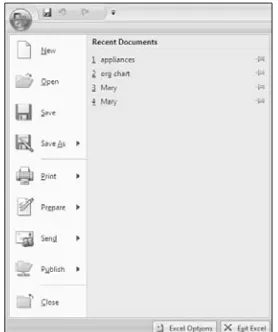
1. Choose Office Button➪Exit Excel, as you see in Figure 1-4.
Optionally, Click the Close button (x).
2. Click Yes or No if prompted to save your workbook. (See “Save a Workbook” later in this chapter.)
Optionally, choose Office ➪Close. The current workbook closes, but the
Excel program remains open.
Figure 1-3:Use the keyboard to select Ribbon commands.
Figure 1-4:Closing Excel releases the program from your computer memory.
➟
7Close Excel
Customize the Quick Access Toolbar
1. Right-click any tool or group title you want to add to the Quick Access toolbar. A menu appears.
2. Choose Add to Quick Access Toolbar. The tool or group icon appears on the Quick Access bar.
3. Right-click an icon on the Quick Access toolbar. A menu appears.
4. Choose Remove from Quick Access Toolbar. The selected item disappears from the Quick Access toolbar.
5. Right-click the Quick Access toolbar and select
Customize the Quick Access Toolbar. The Excel Options dialog box, seen in Figure 1-5, appears.
6. Open the Choose Commands From drop-down menu and select a tab name. Excel displays a list of available features.
7. Select a feature and click the Add button. The selected feature appears on the right panel. Click OK.
Change Status Bar Indicators
1. Right-click anywhere along the status bar at the bottom of the window. Excel opens the Status Bar Configuration menu.
2. To activate an inactive feature, click it. This automati-cally adds a check mark and displays the feature’s status. In Figure 1-6, the Caps Lock feature is on, and now the status bar shows the Caps Lock status.
3. To deactivate any active feature, click it.
Figure 1-5:You can select any Excel options to add to the Quick Access toolbar.
Figure 1-6:Customize what you see along the Excel status bar.
➟
8Chapter 1: Working with Excel Files
Create a New Excel File
1. Click the Office Button.
2. Choose New. The New Workbook dialog box opens. (See Figure 1-7.)
3. Click Blank Workbook.
4. Click the Create button. Excel creates a blank workbook based on the default template.
See Chapter 8, “Changing Worksheet Views,” for more information about Excel templates.
Optionally, press Ctrl+N to create a new workbook without opening the New Workbook dialog box.
Save a Workbook
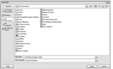
1. Choose Office Button➪Save or click the Save button on the Quick Access toolbar. The Save As dialog box appears, as shown in Figure 1-8.
The Save As dialog box only appears the first time you save a file.
2. By default, Excel saves your files in the My Documents folder. If you want to save your file in a different folder, select that folder from the Save In drop-down list.
3. In the File Name text box, type a descriptive name for the file.
4. Click the Save button. Excel saves the workbook in the location with the name you specified.
Filenames cannot contain asterisk, slash, blackslash, or question mark characters.
Figure 1-7:Excel names each new workbook incrementally such as Workbook 2 or Workbook 3.
Figure 1-8: Choose a folder and filename for your Excel workbook.
➟
9Save a Workbook
Save a Workbook in a
Different Format
1. Choose Office Button➪Save As. The Save As dialog box appears.
2. Select the folder where you want to save the file from the Save In drop-down list.
3. In the File Name text box, type a descriptive name for the file.
4. Open the Save As Type drop-down menu. A list of file formats appears.
5. Choose one of the 26 different file formats. Files saved in the Excel 2007 format have a .xlsx extension, whereas files created in earlier versions of Excel have a .xls extension.
6. Click Save. Depending on the format you choose, Excel may prompt you for additional information.
Open an Existing Excel File
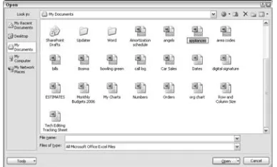
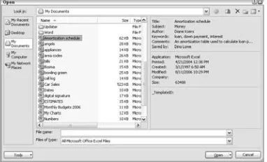
1. Choose Office Button➪Open. The Open dialog box, seen in Figure 1-10, appears.
2. If necessary, select the appropriate folder from the Look In drop-down list. Then select the file you want to open.
Open the Files of Type drop-down menu to display files saved in other formats.
3. Click the Open button. The workbook appears in the Excel workspace, ready for you to edit.
If the file you open was created in a previous version of Excel, the words Compatibility Mode appear on the title bar next to the document name.
Figure 1-9:Excel warns you of compatibility conflicts.
Figure 1-10:Open a previously created Excel file.
Excel displays recently used files on the right side of the Office Button menu. Click any listed filename to quickly open it.
➟
10Chapter 1: Working with Excel Files
Rename a File
1. Open Excel, but not the file you want to rename. Choose Office Button➪Open. The Open or Save As dialog box appears.
Optionally, choose Office Button➪Save As and continue as described.
2. If necessary, click the Look In list and navigate to the folder containing the file you want to delete.
3. Right-click the file. Do not double-click the file because double-clicking the file opens it.
4. Choose Rename from the shortcut menu. (See Figure 1-11.) The original filename becomes highlighted.
5. Type the new file name. Filenames cannot contain aster-isk, slash, blackslash, or question mark characters.
6. Press Enter when you are finished typing.
7. Click the Cancel button to close the Open dialog box.
Figure 1-11:Change the name of an existing Excel workbook.
➟
11Rename a File
Delete a File
1. Open Excel, but not the file you want to delete. Choose Office Button➪Open or Office➪Save As. Either the Open or Save As dialog box appears.
2. If necessary, click the Look In list and navigate to the folder containing the file you want to delete.
3. Right-click on the unwanted file. Do not double-click the file.
4. Choose Delete from the shortcut menu. (See Figure 1-12.) A confirmation message appears.
5. Click Yes. Excel deletes the file.
6. Click the Cancel button to close the Open or Save As dialog box.
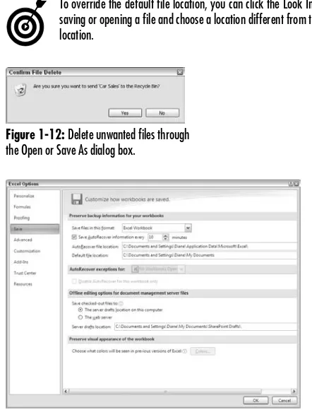
Set the Default File Locations
1. Click the Office Button and click Excel Options. (It’s located at the bottom of the Office list.) The Excel Options dialog box opens.
2. From the options on the left side of the dialog box, click the Save category. You see the options shown in Figure 1-13.
3. In the Default file location, enter the data path to the place where you want to save most of your files. Click OK.
By default, Excel saves your files in the My Documents folder stored on your local hard drive, but your company may have another loca-tion where it wants you to keep most of your Excel files. An exam-ple might be G:\COMPANY DOCUMENTS\DIANE
To override the default file location, you can click the Look In list when saving or opening a file and choose a location different from the default location.
Figure 1-12:Delete unwanted files through the Open or Save As dialog box.
Figure 1-13:Customize to determine where Excel stores your workbooks.
➟
12Chapter 1: Working with Excel Files
Specify Workbook Properties
1. Click the Office Button and click Prepare. A list of options appears.
2. Click Properties. The Document Information Panel appears.
3. Enter identifying information such as the author’s name, subject, or a list of keywords. See Figure 1-14.
Excel automatically adds statistical information such as the work-book’s original creation date, the last time it was printed or modi-fied, and the workbook size.
4. Click the Close box to close the Document Information Panel.
View Workbook Properties
1. Choose Office Button➪Open. The Open dialog box appears.
2. If necessary, click the Look In list and navigate to the folder containing the file you want to delete.
3. Click the Views button drop-down arrow to display a Views shortcut menu or click the Views button itself to cycle through the available views.
4. Choose Properties. The Open window splits into two panels like the ones you see in Figure 1-15.
5. Click a file name. Excel displays the workbook proper-ties in the right panel.
6. Click OK to open the file or Cancel to close the Open dialog box.
Figure 1-14:Enter information to identify your workbook.
Figure 1-15:View the workbook’s properties and file statistics.
➟
13View Workbook Properties
➟
14Chapter 1: Working with Excel Files
Entering Spreadsheet
Data
E
xcel is a huge grid made up of columns and rows. If you’ve used previ-ous versions of Microsoft Excel, you know the new spreadsheet is larger than ever. A single worksheet now contains 16,384 columns (stretching from column A to column XFD) and 1,048,576 rows.You enter three types of data in the cells:
➟
Labelsare traditionally descriptive pieces of information such as names, months, or other identifying statistics, and they usually include alphabetic characters.➟
Valuesare generally raw numbers or dates.➟
Formulasare instructions for Excel to perform calculations. In the first part of this chapter, I show you how to easily enter labels and values into your worksheet. But, alas, human beings sometimes make mis-takes or change their minds. So I also show you how to delete incorrect entries, duplicate data, or move it to another area of the worksheet. You even discover an Excel feature that prevents worksheet cells from accepting incor-rect data.2
Get ready to . . .
➟
Change the Active Cell...16➟
Undo Data Entry...18➟
Enter, Edit, or Delete Cell Data ...17➟
Select Cells ...19➟
Move, Copy and Paste Data ...20➟
Transpose Data ...20➟
Extend a Series with AutoFill ...21➟
Name and Use a Range of Cells ...22➟
Manage Range Names ...23➟
Validate Data Entry...24➟
Enter Data in Validated Cells ...25➟
Locate Cells with Data Validation ...25➟
Chapter
Change the Active Cell
1. Open a spreadsheet in Excel. The formula bar displays the active cell location. Columns display the letters from A to XFD and rows display numbers from 1 to 1048576. A cell address is the intersection of a column and a row such as D23 or AB205.
2. Move the focus to an adjacent cell with one the follow-ing techniques:
• Down:Press the Enter key or the down arrow key. • Up:Press the up arrow key.
• Right:Press the right arrow key • Left:Press the left arrow key.
3. To move to a cell farther away, use one of these techniques:
• Click the mouse pointer on any cell to move the active cell location to that cell. You can use the scroll bars to see more of the worksheet. In Figure 2-1, the cell focus is in cell E10.
• Choose Home ➪Editing➪Find & Select➪Go To. The Go To dialog box displays, as shown in Figure 2-2. In the Reference box, enter the address of the cell you want to make active and then click OK.
Press the F5 key to display the Go To dialog box.
• Press Ctrl + Home. Excel jumps to cell A1.
• Press Ctrl + End. Excel jumps to the lower-right cell of the worksheet.
• Press Ctrl + PageDown or Ctrl + PageUp. Excel moves to the next or previous worksheet in the workbook.
Figure 2-1:A black border surrounds the active cell.
Figure 2-2:Specify a cell address in the Go To box.
➟
16Chapter 2: Entering Spreadsheet Data
Enter Cell Data
1. Type the label or value in the desired cell.
2. Press Enter. The data is entered into the current cell and Excel makes the next cell down active. (See Figure 2-3.) How Excel aligns the data depends on what it is:
To enter a value as a label, type an apostrophe before the value.
• Label: Excel aligns the data to the left side of the cell. If the descriptive information is too wide to fit, Excel extends that data past the cell width if the next cell is blank. If the next cell is not blank, Excel displays only enough text to fit the display width. Widening the column displays additional text.
• Whole value:If the data is a whole value such as 34 or 5763, Excel aligns the data to the right side of the cell.
• Value with a decimal: If the data is a decimal value, Excel aligns the data to the right side of the cell, includ-ing the decimal point, with the exception of a trailinclud-ing 0. For example, in Figure 2-4, if you enter 246.75,then
246.75displays; if you enter 246.70, however, 246.7
displays. (See Chapter 5 to change the display appear-ance, column width, and alignment of your data.)
If a value displays as scientific notation or number sign, it means the value is too long to fit into the cell. You need to widen the col-umn width.
• Date: If you enter a date, such 12/3, Dec 3, or 3 Dec, Excel automatically returns 03-Dec in the cell, but the formula bar displays 12/03/2006. Figure 2-4 also illustrates an example of date entry. See Chapter 5 to change the date format.
Figure 2-3:Enter labels or values into a cell.
Figure 2-4:Entering values.
➟
17Enter Cell Data
Undo Data Entry
1. Enter text into a spreadsheet.
2. To undo any actions or correct any mistakes you make when entering data, perform one of the following:
• Choose Undo from the Quick Access toolbar.
• Press Ctrl+Z.
3. Keep repeating your favorite undo method until you’re back where you want to be.
4. To undo several steps at once, click the arrow on the Undo icon and select the step from which you want to begin the Undo action. (See Figure 2-5.)
Edit or Delete Cell Data
1. To delete the entire contents of a cell, use one of the fol-lowing methods:
• Choose Home➪Editing➪Clear. • Press the Delete key.
2. To edit the cell contents, use one of these methods: • Delete the contents and retype new cell information.
• Press F2 and edit the cell contents from the formula bar.
• Double-click the cell contents and edit the cell con-tents from the cell. (See Figure 2-6.)
Figure 2-5:Select the steps you want to reverse.
Figure 2-6:Edit cell contents without having to start over.
To repeat your last action, click the Redo icon on the Quick Access tool-bar or press Ctrl+Y. You can’t repeat some actions, however. If you clear the wrong cell, use the Undo command.
➟
18Chapter 2: Entering Spreadsheet Data
Select Multiple Cells
1. Click the first cell in the group you want to select.
2. Depending on the cells you want to select, perform one of the following actions.
• To select sequential cells, hold down the Shift key and select the last cell you want. All cells in the selected area are highlighted, with the exception of the first cell. (Don’t worry; it’s selected, too.) Figure 2-7 shows a sequential area selected from cell B4to cell F15. Notice the black border surrounding the selected area.
• To select nonsequential cells, hold down the Ctrl key and click each additional cell you want to select. Figure 2-8 shows the nonsequential cells A4, C7, andE4 through E9selected.
• To select a single entire column, click a column heading.
• To select multiple columns, drag across multiple col-umn headings.
• To select a single entire row, click the row number.
• To select multiple rows, drag across multiple row numbers.
• To select the entire worksheet, click the small gray box located to the left of column A and above row 1. Optionally, you can select all cells in a worksheet by pressing Ctrl + A
When making nonsequential cell selections, you can include entire rows and entire columns along with individual cells or groups of cells.
Figure 2-7:A sequential cell selection.
Figure 2-8:Non-sequential cells selected.
Click any nonselected cell to clear the selection.
Optionally, click and drag the mouse over a group of cells to select a sequential area.
➟
19Select Multiple Cells
Copy and Paste Data
1. Select the area of data you want to copy.
2. Choose Home➪Copy. A marquee(which looks like marching ants) surrounds the cells (see Figure 2-9).
3. Click the cell to which you want to copy the selected area.
4. Choose Home➪Paste. The selected cells are pasted into the new location.
5. Paste the cells into another location or press Esc to can-cel the marquee.
Choose Home➪Cut and then Home➪Paste to move (instead of
duplicate) the selected cells to a different location.
Optionally, press Ctrl+C to copy the selected cells; Ctrl+X to cut the selected cells, or Ctrl+V to paste the selected cells.
Transpose Data
1. Select the cells you want to transpose.
2. Choose Home➪Copy.
The Transpose feature will not work if you choose Cut instead of Copy.
3. Click the cell where you want the transposed cells to begin.
4. On the Home tab of the Ribbon, click the down arrow below Paste. A menu of options appears.
5. Choose Transpose. As you see in Figure 2-10, Excel copies the selected cells into the new area, transposing rows into columns or columns into rows.
Figure 2-9:Marching ants form around a copied area.
Figure 2-10:Reverse the flow of data by transposing cells.
➟
20Chapter 2: Entering Spreadsheet Data
Extend a Series with AutoFill
1. Type the first cell of data with data such as a day or month, such as Wednesday or September. AutoFill works with days of the week, months of the year, or yearly quarters such as 2nd Qtr. You can enter the entire word or you can enter the abbreviated form (Wed or Sep).
2. Press Enter.
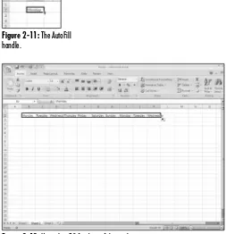
3. Position the mouse pointer on the small black box at the lower-right corner of the data cell. Your mouse pointer turns into a small black cross. (See Figure 2-11.)
To AutoFill a series of numbers, enter two values in two adjacent cells, such as 1 and 2 or 5 and 10. Select both cells, and then use the AutoFill box to highlight cells. Excel continues the series as 3, 4, 5, or 5, 10, 15, and so forth.
4. Drag the small black box across the cells you want to fill. You can drag the cells up, down, left, or right.
5. Release the mouse. Excel fills in the selected cells with a continuation of your data. Figure 2-12 shows how Excel fills in the cells with the rest of the days of the week.
If you use AutoFill on a single value or a text word, Excel duplicates it. For example, if you use AutoFill on a cell with the word Apple, all filled cells contain Apple.
To quickly use the AutoFill, highlight the cell that has the data and the cells you want to fill and then double-click the fill-handle. Chapter 10 includes instructions for creating your own customized list. Autofill can enter lists you often use, such as sales rep names or product types.
Figure 2-11:The AutoFill handle.
Figure 2-12:Using AutoFill for days of the week.
➟
21Extend a Series with AutoFill
Name a Range of Cells
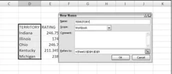
1. After selecting the cells you want to name, click Formulas➪Named Cells➪Name a Range. The New Name dialog box appears. (See Figure 2-13.)
2. In the Name text box, type up to a 255-character name for the range. Range names are not case-sensitive; how-ever, range names must follow these conventions:
• The first character must be a letter, an underscore, or a backslash.
• No spaces are allowed in a range name.
• Do not use a name that is the same as a cell address. For example, you can’t name a range AB32.
3. Click OK.
Optionally, enter a range name into the Name box located at the left end of the Formula bar. You can jump quickly to a named range by clicking the down arrow in the Name box and selecting the range name.
Use Named Ranges
1. Click the down arrow in the Name box. A list of named ranges appears. (See Figure 2-14.)
2. Select the range name you want to access. Excel high-lights the named cells.
Optionally, choose Home➪Editing➪Find & Select➪Go To.
Double-click on the range name you want to access.
Figure 2-13:For faster formula entry, use range names.
Figure 2-14:Quickly locate an area by using a range name.
➟
22Chapter 2: Entering Spreadsheet Data
Manage Range Names
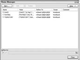
1. Choose Formulas➪Named Cells➪Name Manager. The Name Manager dialog box, shown in Figure 2-15, appears.
Excel automatically adds tables to the Name Manager. See Chapters 6 and 10 for more on working with tables.
2. Select one of the following options.
• Click the New button, which displays the New Name dialog box in which you can enter a range name and enter the cell location it refers to.
Instead of typing the range cell locations, click the Collapse button, which moves aside the New Name dialog box. You can then use your mouse to select the desired cells. Press Enter or click the Collapse button again to return to the New Name dialog box.
• Click an existing range name and then click the Edit button, which displays the Edit Name dialog box shown in Figure 2-16. Use this dialog box to change the range name or the range cell location reference.
• Click an existing range name and then click the Delete button. A confirmation message appears, making sure you want to delete the range name.
If you have a lot of range names, you can click the Filter button and elect to display only the items meeting selected criteria.
3. Click the Close button to close the Name Manager dia-log box.
Figure 2-15:Use the Name Manager to add, edit, or delete range names.
Figure 2-16:Edit a range name and cell location.
➟
23Manage Range Names
Validate Data Entry
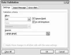
1. Select the cell or cells you want Excel to validate. Next, choose Data➪Data Tools➪Validation. The Data Validation dialog box displays.
2. In the Settings tab, open the Allow drop-down list and choose the type of validation, such as:
• Values such as Whole Number or Decimal, where you specify the upper and lower limits of allowable data values.
• Lists such as a list you define, a range of cells in the existing worksheet, or a named range. (See Figure 2-17.)
• Dates or Times, where you specify ranges or limita-tions such as greater than or less than or even a spe-cific date.
• Text Length, where the number of characters in the data must be within the limits that you specify.
3. If necessary, display the Data drop-down list and select criteria such as Between, Greater Than, and so on.
4. Select criteria such as maximum and minimum values, or specify a data location. Enter values or cell addresses. Precede a value with an equal sign (=) to specify a range name.
5. From the Input Message tab, optionally enter a comment to display whenever someone clicks the validated cell.
6. On the Error Alert tab, choose from the Style drop-down list whether Excel warns you or completely stops you from entering an invalid entry. (See Figure 2-18.)
7. Click OK.
Figure 2-17: Create a list of acceptable options or select one from the worksheet.
Figure 2-18:Determine the action to take when an invalid data entry occurs.
When creating a list, if you want the available choices to appear when the cell is selected, make sure to select the In-Cell drop-down check box. On the Error Alert tab of the Data Validation dialog box, you can cus-tomize the error message Excel displays if an invalid entry is entered.
➟
24Chapter 2: Entering Spreadsheet Data
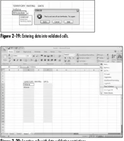
Enter Data in Validated Cells
1. Click a cell that has a validation requirement.
2. Type data into the cell.
3. Press Enter. One of two things happens:
• If the data meets the validation rules, Excel accepts the entry and moves to the next cell down.
• If the data does not meet the validation rules, Excel displays an error message similar to the one you see in Figure 2-19.
4. Depending on the setting you selected on the Error Alert tab in the Data Evaluation dialog box, choose an option:
• Stop: Choose Retry or Cancel
• Warning: Choose Yes or No or Cancel
• Information: Choose OK or Cancel
Locate Cells with Data Validation
1. To have Excel highlight all cells that have data validation, select one of the following methods (see Figure 2-20):
• Choose Home➪Editing➪Find & Select➪Data Validation.
• Choose Home➪Editing➪Find & Select➪Go To Special. Select the Data Validation option, choose All, and then click OK.
2. Click any cell to deselect the highlighted cells.
To remove data validation, choose Data➪Data Tools➪Data Validation. From the Data Validation dialog box, click the Clear All button and then click the OK button.
Figure 2-19:Entering data into validated cells.
Figure 2-20:Locating cells with data-validation restrictions.
➟
25Locate Cells with Data Validation
➟
26Chapter 2: Entering Spreadsheet Data
➟
Building Formulas
T
his chapter is all about the math. With Excel, you can create formulas to perform calculations. The calculations can be simple, such as adding 2 plus 3, or they can be extremely complex, such as those used to calculate depreciation. But don’t despair; you don’t have to do most of the work. Excel includes more than 335 built-in calculations, which are calledfunctions, in 11 different categories. Functions contain arguments, which appear in parentheses following the function’s name. The arguments are the details you provide to Excel to indicate which numbers to calculate in the function. Some functions require several arguments to function correctly, but again I say, don’t worry; Excel contains a Function Wizard to walk you through the entire process.
The primary tasks in this chapter include:
➟
Creating simple and complex formulas by typing them into a cell.➟
Analyzing data with Excel’s time-saving functions.➟
Creating cell ranges separated by colons for a sequential cell selection or by commas to list specific cell locations.➟
Evaluating formula errors and locating a cell’s precedents and dependents.3
Get ready to . . .
➟
Create Simple Formulas ...28➟
Create Compound Formulas...29➟
Add Numbers with AutoSum ...30➟
Find an Average Value ...30➟
Copy and Edit Formulas ...31➟
Define an Absolute Formula ...32➟
Copy Values Using Paste Special ...32➟
Build a Formula withthe Function Wizard ...33
➟
Generate an IF Statement Formula ...34➟
Troubleshoot Formula Errors ...35➟
Identify Formula Precedentsand Dependents ...36
➟
Chapter
Create Simple Formulas
with Operators
1. Enter values in two different cells; remember, however, formulas do not need to reference cell addresses. They can contain actual numbers.
2. In the cell where you want to perform the calculation for the two values, type an equal sign (=). All Excel for-mulas begin with an equal sign.
3. Click or type the first cell address or type the first value you want to include in the formula. In the example in Figure 3-1, I’m adding two cell references (B5 and B6) together.
Excel displays a color border that surrounds the cell reference you enter.
4. Type an operator. Operators can include: • The plus sign (+)
• The minus sign (–)
• The asterisk (*) to multiply
• The slash (/) to divide
• The percentage symbol (%) • The exponentiation symbol (^)
5. Type the second cell address or the second value you want to include in the formula.
6. Press Enter and Excel displays the results of the calcula-tion in the selected cell. (See Figure 3-2.)
The formula bar at the top displays the actual formula.
Formulas can have multiple references. For example, =B5+B6+B6+B8 is a legitimate formula. Formulas with multiple operators are called compound formulas.
Figure 3-1:All formulas begin with an equal sign.
Figure 3-2:A simple formula.
➟
28Chapter 3: Building Formulas
Create Compound Formulas
1. Type values in three or more different cells.
2. Select the cell where you want the formula.
3. Type the equal sign and then the first cell reference.
4. Type the first operator and then the second cell reference.
5. Type the second operator and then the third cell reference.
Compound formulas are not limited to three references, and you can use cell references multiple times in a compound formula.
6. Press Enter. Excel displays the results of the calculation in the selected cell. The actual formula appears in the formula bar. (See Figure 3-3.)
If you were paying attention in your high school algebra class, you might remember the Rule of Priorities. In a compound formula, Excel calculates multiplication and division before it calculates addi-tion and subtracaddi-tion. This means that you must include parentheses for any portion of a formula you want calculated first. As an exam-ple, in Figure 3-4, you see that the formula 3+5*2gives a result of 13, but (3+5)*2gives a result of 16. You can include range names in formulas such as =D23* CommissionRate where a specific cell is named
CommissionRate. See Chapter 2 about using range names.
Compound formulas can have multiple combinations in parentheses and can contain any combination of operators and references. A for-mula might read ((B5+C5)/2)*SalesTax. This formula adds B5and C5, divides that result by 2, and then mul-tiplies that result times the value in the cell named SalesTax.
A great tool to review formulas is the capability to display the actual for-mula in the worksheet rather than the forfor-mula result. Choose Forfor-mulas➪
Formula Auditing➪Show Formulas. Click the Show Formulas button
again to return to the formula result.
Figure 3-3:A compound formula.
Figure 3-4:The Rule of Priorities in action.
➟
29Create Compound Formulas
Add Numbers with AutoSum
1. Click the cell beneath a sequential list of values.
2. Click Formulas➪Function Library➪AutoSum. Excel places a marquee (marching ants) around the cells directly above the current cell. (See Figure 3-5.)
3. Press the Enter key to display the sum total of the selected cells.
Find an Average Value
1. After selecting the cell beneath a sequential list of val-ues, click the arrow beneath the AutoSum button. Excel displays a list of calculation options, including (see Figure 3-6):
• Average. Calculated by adding a group of numbers and then dividing by the count of those numbers.
• Count Numbers. Counts the number of cells in a specified range that contain numbers.
• Max. Determines the highest value in a specified range. • Min. Determines the lowest value in a specified range.
2. Choose Average. A marquee appears around the group of cells. Highlight a different group of cells if necessary.
3. Press Enter. The selected cell displays the average value of the cell group.
Figure 3-5:Using the AutoSum function.
Figure 3-6:Selecting the Average function.
If the cells directly above the current cell have no values, Excel selects the cells directly to the left of the current cell. If you want to add a group of different cells, highlight them.
The formula bar displays the formula beginning with the equal sign and the word SUM. The selected cells appear in parentheses, the first and last cells separated by a colon.
➟
30Chapter 3: Building Formulas
Copy Formulas with AutoFill
1. Position the mouse on the AutoFill box in the lower-right corner of a cell with a formula. Make sure the mouse pointer turns into a black cross.
2. Click and drag the AutoFill box to include the cells to which you want to copy the formula. (See Figure 3-7.) The AutoFill method of copying formulas is helpful if you’re copying a formula to surrounding cells.
Copied formulas are slightly different than the originals because of the relative change in position. For example, if the formula in cell
D23is B23+C23and you copy the formula to the next cell down, to cell D24, Excel automatically changes the formula to
B24+C24. If you do not want the copied formula to change, you must make the originating formula an absolute formula (see the “Define an Absolute Formula” section later in this chapter).
Edit a Formula
1. Double-click the cell containing the formula you want to edit. The cell expands to show the formula instead of the result. (See Figure 3-8.)
Optionally, press the F2 key to expand the formula so you can edit it.
2. Use the arrow keys to navigate to the character you want to change.
3. Using the Backspace key, delete any unwanted characters and type any additional characters.
4. Press Enter.
Press the Delete key to delete the entire formula and start over.
Figure 3-7:Using AutoFill to duplicate a formula.
Figure 3-8:Edit a formula.
➟
31Edit a Formula
Define an Absolute Formula
1. To prevent a formula from changing a cell reference as you copy it to a different location, you lock in an absolute cell reference using one of these methods:
• Lock in a cell location: Type a dollar sign in front of both the column reference and the row reference (as in $C$2). If the original formula in cell F5 is =E5*$C$2, and you copy the formula to cell F6, the copied formula reads E6*=$C$2instead of E6*C3, which is how it would read were it not absolute. (See Figure 3-9.)
• Lock in the row or column location only:Type a dollar sign in front of the column reference ($C2) or in front of the row reference (C$2).
2. Copy the formula, as needed, to other locations. Notice that the absolute cell reference in the original formula remains unchanged in the copied formulas.
Copy Values Using Paste Special
1. Select a cell (or group of cells) containing a formula and then choose Home➪Clipboard➪Copy. A marquee appears around the selected cell.
2. Select the cell where you want the answer; then click the arrow under the Paste button on the Home tab.
3. Choose Paste Special. The Paste Special dialog box, shown in Figure 3-10, appears.
4. Select the Values option.
5. Click OK.
Figure 3-9:A formula containing an absolute reference.
Figure 3-10:Paste only the value, not the formula with the Paste Special feature.
➟
32Chapter 3: Building Formulas
Build a Formula with
the Function Wizard
1. Select the cell where you want to enter a function.
2. Click Insert Function, which is the icon located in the lower-right corner of the Function Library group on the Formulas tab. The Insert Function dialog box appears.
3. Select a function category from the Or Select a Category drop-down list. (See Figure 3-11.)
To make the functions easier to locate, Excel separates them into categories including Financial, Date, Math & Trig, Statistical, Lookup and Ref, Database, Text, Logical, Information, and — new to Excel 2007 — the Engineering and Cube categories. For example, the Sum function is in the Math category, while the Average, Count, Max, and Min are Statistical functions. Functions that calculate a payment value are considered Financial functions.
4. Select a function name from the Select a Function list. A brief description of the function and its arguments appears under the list of function names.
5. Click OK. The Function Arguments dialog box displays. The contents of this dialog box depend on the function you’ve selected. Figure 3-12 shows the PMT function that calculates a loan payment based on constant pay-ments and interest.
6. Type the first argument amount or cell reference or click the cell in the worksheet. If you click the cell, Excel places a marquee around the selected cell.
7. Press Tab to move to the next argument.
8. Type or select the second argument.
9. Repeat Steps 7 and 8 for each necessary argument.
10. Click OK. Excel calculates the result.
Arguments in bold type are required. Those in normal type are optional.
Figure 3-11:Select from more than 335 built-in functions.
Figure 3-12:Specifying arguments for the PMT function.
➟
33Build a Formula with the Function Wizard
Generate an IF Statement Formula
1. Select a cell where you want to show the formula result.
2. Type the equal sign and then the word IF.
3. Type an open parenthesis (.
4. Begin the first argument by referencing the cell you want to check. For example, if you want to check whether cell B10 is greater than 100, type B10.
5. Type an operator such as equal to (=), greater than (>), or less than (<).
6. Type the value or cell reference you want to compare against.
7. Type a comma to begin the second argument.
8. Type what you want Excel to do if the first argument is true. If you want Excel to display a value or cell value, type the value or cell reference; but if you want Excel to display text, enclose the text in quotation marks. (See Figure 3-13.)
9. Type a comma to begin the third and final argument.
10. Type what you want Excel to do if the first argument is not true. As before, type the value, cell reference, or text you want Excel to display.
11. Press the Enter key. Excel displays the results of the analysis in the selected cell. In Figure 3-14, you see the result of NO I CAN’Tin cell B8 because the payment amount was not less than the limit.
Arguments in an IF statement can also contain formulas.
Figure 3-13:Entering IF statement arguments.
Figure 3-14:The results of a statement that was NOT TRUE.
➟
34Chapter 3: Building Formulas
Troubleshoot Formula Errors
1. Choose Formulas➪Formula Auditing➪Error Checking. If Excel finds potentialformula errors in your worksheet, it jumps to the cell containing the error and displays the Error Checking dialog box shown in Figure 3-15. If the worksheet contains no errors, Excel displays a message box saying the error-checking is complete. Here are just a few of the error types Excel might locate:
• DIV/0!: Divide by zero error. This error means the formula is trying to divide by either an empty cell or one with a value of zero. Make sure all cells referenced in the division have a value other than zero in them.
• #VALUE!:This means the formula references an invalid cell address. For example, text is in a cell where the formula is expecting to find a value. You might also see this error if you delete a value in a cell that was used in a formula. Locate and correct the invalid cell reference.
• NAME#: This occurs when Excel doesn’t recognize text in a formula, perhaps because of a misspelling of a range name. Make sure the name actually exists and is spelled correctly. Also verify the spelling of the function name.
• Circular:This means that the formula in a cell is referring to itself. Locate the circular reference and edit the formula so it does not include itself. Figure 3-16 shows a circular reference.
• Number Stored as Text: This means a cell contains what looks like a value, but the content is stored as text. Verify that you did intend to store the value as a text entry.
Figure 3-15:Let Excel find potential formula errors.
Figure 3-16:Circular References: Where a formula refers to its own cell address.
➟
35Troubleshoot Formula Errors
• Formula Omits Adjacent Cells:This means a formula refers to a group of cells that have numbers adjacent to it. Study the formula to make sure you didn’t forget to include additional cell refer-ences in the formula.
2. Perform one of the following steps, depending on the error type:
• Click in the cell and edit the formula as needed. Click Resume when you are finished.
• Click Ignore Error to jump to the next potential problem.
• Click an option, if available, to allow the Error Checking dialog box to assist you with repairing the problem.
3. Click Next to review the next problem area. When the error-check process is complete, Excel displays a message box.
4. Click OK.
Identify Formula Precedents
and Dependents
1. Select a cell that contains a formula or one that is refer-enced in one or more formulas.
2. Choose Formulas➪Formula Auditing➪Trace Precedents or Trace Dependents. Excel displays one or more blue arrows pointing out either precedents or, as shown in Figure 3-18, dependents.
3. Click Remove Arrows. The blue arrows disappear.
Figure 3-17:Show formulas instead of results.
Figure 3-18:Tracer arrows indicate formula precedents or dependents.
To help you determine the nature or origin of the problem, some error messages have a Show Calculation Steps button to display the logic behind the formula.
Another great troubleshooting tool is the capability to display the actual formula, instead of the result, in the worksheet. Choose Formulas➪Formula Auditing➪Show Formulas. Click the same button
again to return to the formula result. (See Figure 3-17.)
Dependent cells are those that are referred to by a formula in another cell. Precedent cells are those that contain formulas that refer to other cells.
➟
36Chapter 3: Building Formulas
➟
Protecting Excel Data
W
orksheets often contain numerical information that is confidential in nature, such as financial or payroll data. In today’s world of elec-tronic snooping, it’s up to you to protect your work against prying eyes. Fortunately, Excel provides a large number of security tools such as password protection, hiding sensitive worksheet areas, or locking data againstunwanted changes.
This chapter is about the security concerns surrounding Excel workbooks. I’ll show you many distinctive protection methods including how to:
➟
Hide all or selected areas of a workbook➟
Specify that users can view a file but not modify it➟
Restrict the access to designated worksheet ranges➟
Mark a file as final to protect it from changes➟
Assign passwords to open or modify a workbook➟
Remove private data from a workbook before sending it on to others.4
Get ready to . . .
➟
Quickly Hide an Open Workbook...38➟
Make a File Read-Only ...38➟
Open a File as Read-Only ...39➟
Mark a Workbook as Final ...39➟
Hide and Unhide Rows and Columns ...40➟
Unlock Cells ...40➟
Protect Worksheets ...41➟
Restrict User Data Entry ...42➟
Enter Data in a Restricted Area ...43➟
Inspect for Private Information ...43➟
Hide Cell Formulas ...44➟
Assign a File Password ...44➟
Chapter
Quickly Hide an Open Workbook
1. Choose View➪Hide. Excel hides the current workbook, leaving the Excel program open and visible. If you have another workbook open, you see that workbook, but not the hidden workbook.
2. Choose View➪Unhide. Excel displays the Unhide dialog box listing all hidden workbooks, as you see in Figure 4-1.
3. Select the workbook you want to unhide.
4. Click OK.
Make a File Read-Only
1. Choose Office Button➪Save As. The Save As dialog box opens.
2. Optionally, select a file location from the Save-in drop-down list.
3. Enter a filename.
4. Click the Tools button. A drop-down menu appears.
5. Choose General Options. The General Options dialog box, shown in Figure 4-2, appears.
6. Click the Read-Only Recommended option.
7. Click OK.
8. Click Save.
Figure 4-1:Hidden workbooks do not even appear on the Windows taskbar.
Figure 4-2:Protect against accidental changes by making a file Read-Only accessible.
The Read-Only option is only a recommendation. Users can save changes to a read-only file by giving it a different name or saving it in a different folder.
➟
38Chapter 4: Protecting Excel Data
Open a File as Read-Only or Copy
1. Choose Office Button➪Open. The Open File dialog box appears.
2. Locate and select the file you want to open.
3. Click the arrow on the Open button. A list of options appears. (Figure 4-3).
4. Choose Open Read-Only or Open as Copy. The file opens.
5. To save any changes to the file, you must choose Home➪Save As and specify a different file name.
If you open a file as a copy and do not use the Save As option, Excel uses the filename “Copy (#) filename” where # represents the copy number and filename is the current filename.
Mark a Workbook as Final
1. Choose Office Button➪Finish➪Mark as Final. The mes-sage box seen in Figure 4-4 appears.
2. Click OK.
3. If you have not yet saved the file, the Save As dialog box appears. Enter the filename and save the file. Otherwise, Excel saves the file and the words Read-Onlyappear next to the filename on the Title bar.
The Mark as Final feature is designed to prevent accidental changes and is not permanent. If you find you need to make changes to the workbook, choose Office Button➪Finish➪Mark as Final again to turn off the Read-Only function.
Figure 4-3:Different approaches to opening your workbook.
Figure 4-4:Marking a workbook as final makes it a read-only file.
➟
39Mark a Workbook as Final
Hide and Unhide Rows and Columns
1. Select the column or row headings you want to hide. If you want to unhide rows or columns, select the row or columns both before and after the hidden rows or columns.
2. Choose Home➪Cells➪Format➪Hide and Unhide. A menu of options appears.
You cannot hide selected cells; only entire columns or rows.
3. Make a selection. In Figure 4-5, notice that columns D & E are hidden and seem to have disappeared.
Unlock Cells
1. Select the cells you want users to be able to modify.
2. Choose Home➪Cells➪Format➪Cells, which displays the Format Cells dialog box.
3. Click the Protection tab, as shown in Figure 4-6.
4. Deselect the Locked option.
5. Click OK.
Optionally, choose Home➪Cells➪Format➪Lock Cells. Because, by default, Excel locks all cells, choosing this option turns the Lock Cells option off. Click the option again to turn on the Lock Cells option.
Figure 4-5:Hide worksheet columns.
Figure 4-6:Unlocked cells can be edited in a protected worksheet.
➟
40Chapter 4: Protecting Excel Data