by Greg Harvey, PhD
Excel
Workbook
FOR
DUMmIES
Excel
Workbook
FOR
DUMmIES
by Greg Harvey, PhD
Excel
Workbook
FOR
DUMmIES
111 River Street Hoboken, NJ 07030-5774
www.wiley.com
Copyright © 2007 by Wiley Publishing, Inc., Indianapolis, Indiana Published by Wiley Publishing, Inc., Indianapolis, Indiana Published simultaneously in Canada
No part of this publication may be reproduced, stored in a retrieval system or transmitted in any form or by any means, electronic, mechanical, photocopying, recording, scanning or otherwise, except as permitted under Sections 107 or 108 of the 1976 United States Copyright Act, without either the prior written permission of the Publisher, or authorization through payment of the appropriate per-copy fee to the Copyright Clearance Center, 222 Rosewood Drive, Danvers, MA 01923, (978) 750-8400, fax (978) 646-8600. Requests to the Publisher for permission should be addressed to the Legal Department, Wiley Publishing, Inc., 10475 Crosspoint Blvd., Indianapolis, IN 46256, (317) 572-3447, fax (317) 572-4355, or online at http://www.wiley.com/go/permissions.
Trademarks:Wiley, the Wiley Publishing logo, For Dummies, the Dummies Man logo, A Reference for the Rest of Us!, The Dummies Way, Dummies Daily, The Fun and Easy Way, Dummies.com, and related trade dress are trademarks or registered trademarks of John Wiley & Sons, Inc. and/or its affiliates in the United States and other countries, and may not be used without written permission. Microsoft and Excel are registered trademarks of Microsoft Corporation in the United States and/or other countries. All other trademarks are the property of their respective owners. Wiley Publishing, Inc., is not associated with any product or vendor mentioned in this book.
LIMIT OF LIABILITY/DISCLAIMER OF WARRANTY: THE PUBLISHER AND THE AUTHOR MAKE NO REPRESENTA-TIONS OR WARRANTIES WITH RESPECT TO THE ACCURACY OR COMPLETENESS OF THE CONTENTS OF THIS WORK AND SPECIFICALLY DISCLAIM ALL WARRANTIES, INCLUDING WITHOUT LIMITATION WARRANTIES OF FIT-NESS FOR A PARTICULAR PURPOSE. NO WARRANTY MAY BE CREATED OR EXTENDED BY SALES OR PROMO-TIONAL MATERIALS. THE ADVICE AND STRATEGIES CONTAINED HEREIN MAY NOT BE SUITABLE FOR EVERY SITUATION. THIS WORK IS SOLD WITH THE UNDERSTANDING THAT THE PUBLISHER IS NOT ENGAGED IN REN-DERING LEGAL, ACCOUNTING, OR OTHER PROFESSIONAL SERVICES. IF PROFESSIONAL ASSISTANCE IS REQUIRED, THE SERVICES OF A COMPETENT PROFESSIONAL PERSON SHOULD BE SOUGHT. NEITHER THE PUB-LISHER NOR THE AUTHOR SHALL BE LIABLE FOR DAMAGES ARISING HEREFROM. THE FACT THAT AN ORGAN-IZATION OR WEBSITE IS REFERRED TO IN THIS WORK AS A CITATION AND/OR A POTENTIAL SOURCE OF FURTHER INFORMATION DOES NOT MEAN THAT THE AUTHOR OR THE PUBLISHER ENDORSES THE INFORMA-TION THE ORGANIZAINFORMA-TION OR WEBSITE MAY PROVIDE OR RECOMMENDAINFORMA-TIONS IT MAY MAKE. FURTHER, READ-ERS SHOULD BE AWARE THAT INTERNET WEBSITES LISTED IN THIS WORK MAY HAVE CHANGED OR DISAPPEARED BETWEEN WHEN THIS WORK WAS WRITTEN AND WHEN IT IS READ.
For general information on our other products and services, please contact our Customer Care Department within the U.S. at 800-762-2974, outside the U.S. at 317-572-3993, or fax 317-572-4002.
For technical support, please visit www.wiley.com/techsupport.
Wiley also publishes its books in a variety of electronic formats. Some content that appears in print may not be avail-able in electronic books.
Library of Congress Control Number: 2007932459 ISBN: 978-0-470-16937-7
Manufactured in the United States of America
Greg Harveyhas authored tons of computer books, the most recent being Grieving For Dummiesand Excel Workbook For Dummies, and the ever-popular Excel 2007 For Dummiesand Excel 2007 All-In-One Desk Reference For Dummies. He started out training business users on how to use IBM personal computers and their attendant computer software in the rough-and-tumble days of DOS, WordStar, and Lotus 1-2-3 in the mid-’80s of the last century. After working for a number of independent training firms, he went on to teach semester-long courses in spreadsheet and database management software at Golden Gate University in San Francisco.
His love of teaching has translated into an equal love of writing. For Dummiesbooks are, of course, his all-time favorites to write because they enable him to write to his favorite audience, the beginner. They also enable him to use humor (a key element to success in the training room) and, most delightful of all, to express an opinion or two about the sub-ject matter at hand.
I’m always very grateful to the many people who work so hard to bring my book projects into being, and this one is no exception. This time, preliminary thanks are in order to Andy Cummings and Katie Feltman for giving me this opportunity to write in this won-derful workbook format.
Some of the people who helped bring this book to market include the following:
Acquisitions, Editorial, and Media Development Project Editor:Linda Morris
Acquisitions Editor:Katie Feltman
Copy Editor:Linda Morris
Technical Editor:Joyce Nielsen
Editorial Manager:Jodi Jensen
Media Development Manager:Laura VanWinkle
Editorial Assistant:Amanda Foxworth
Sr. Editorial Assistant:Cherie Case
Cartoons:Rich Tennant (www.the5thwave.com)
Composition Services
Project Coordinator: Jennifer Theriot
Layout and Graphics: Carrie Foster, Denny Hager, Stephanie D. Jumper
Proofreaders: Broccoli Information Management, Christy Pingleton
Indexer: Broccoli Information Management
Anniversary Logo Design:Richard J. Pacifico
Publishing and Editorial for Technology Dummies
Richard Swadley,Vice President and Executive Group Publisher
Andy Cummings,Vice President and Publisher
Mary Bednarek,Executive Acquisitions Director
Mary C. Corder,Editorial Director
Publishing for Consumer Dummies
Diane Graves Steele,Vice President and Publisher
Joyce Pepple,Acquisitions Director
Composition Services
Gerry Fahey,Vice President of Production Services
Introduction ...1
Part I: Creating Spreadsheets ...7
Chapter 1: Getting Familiar with the Excel 2007 Interface ...9
Chapter 2: Entering the Spreadsheet Data ...19
Chapter 3: Formatting the Spreadsheet ...37
Chapter 4: Printing Spreadsheet Reports ...57
Chapter 5: Modifying the Spreadsheet...77
Part II: Using Formulas and Functions ...101
Chapter 6: Building Formulas...103
Chapter 7: Copying and Correcting Formulas...123
Chapter 8: Creating Date and Time Formulas ...145
Chapter 9: Financial Formulas and Functions...153
Chapter 10: Using Math Functions...163
Chapter 11: Using Common Statistical Functions ...175
Chapter 12: Using Lookup Functions ...183
Chapter 13: Using Logical Functions ...193
Chapter 14: Text Formulas and Functions...205
Part III: Working with Graphics...213
Chapter 15: Charting Spreadsheet Data...215
Chapter 16: Adding Graphics to Spreadsheets ...229
Part IV: Managing and Securing Data...251
Chapter 17: Building and Maintaining Data Lists...253
Chapter 18: Protecting the Spreadsheet ...275
Part V: Doing Data Analysis...287
Chapter 19: Performing What-If Analysis...289
Chapter 20: Generating Pivot Tables...303
Part VI: Macros and Visual Basic for Applications ...319
Chapter 21: Using Macros...321
Chapter 24: Top Ten Tips for Using Excel Like a Pro ...349
Introduction...1
Introduction ...1
About This Book ...1
Conventions Used in This Book...1
Foolish Assumptions...2
How This Book Is Organized ...2
Part I: Creating Spreadsheets ...3
Part II: Using Formulas and Functions ...3
Part III: Working with Graphics ...3
Part IV: Managing and Securing Data ...4
Part V: Doing Data Analysis ...4
Part VI: Macros and Visual Basic for Applications ...4
Part VII: The Part of Tens...4
Using the Practice Material on the CD-ROM ...4
Icons Used in This Book ...5
Where to Go from Here ...6
Part I: Creating Spreadsheets...7
Chapter 1: Getting Familiar with the Excel 2007 Interface ...9
Identifying the Parts of the Excel Display Screen...9
Selecting Commands on the Office Menu...11
Selecting Commands from the Ribbon ...12
Selecting Commands on the Quick Access Toolbar...14
Customizing the Quick Access toolbar ...14
Adding more commands to the Quick Access toolbar ...15
Chapter 2: Entering the Spreadsheet Data...19
Launching Excel...19
Opening a New Workbook ...20
Moving Around the Workbook...23
Moving within the displayed area ...23
Moving to a new area of the worksheet ...24
Moving to a different sheet in the workbook ...26
Selecting Cell Ranges ...27
Making Cell Entries...28
Entering data in a single cell ...29
Entering data in a cell range...31
Filling in a data series with the Fill handle ...32
Copying a formula with the Fill handle ...33
Chapter 3: Formatting the Spreadsheet ...37
Resizing Columns and Rows ...37
Making column widths suit the data ...38
Manipulating the height of certain rows...39
Cell Formatting Techniques ...40
Formatting cells with the Ribbon’s Home tab...40
Formatting cells with the Format Cells dialog box...45
Using cell styles ...51
Using conditional formatting...52
Hiding Columns and Rows...55
Chapter 4: Printing Spreadsheet Reports...57
Previewing Pages in the Worksheet Area ...57
Adjusting Page Breaks...59
Adding Headers and Footers...61
Adding Print Titles to a Report...64
Modifying the Print Setting for a Report ...66
Printing All or Part of the Workbook...69
Printing a range of cells ...69
Printing the entire workbook ...70
Printing charts in the spreadsheet ...72
Printing the spreadsheet formulas ...74
Chapter 5: Modifying the Spreadsheet ...77
Finding and Identifying the Region That Needs Editing ...77
Selecting the Ranges to Edit...80
Editing Data Entries...82
Catching Errors with Text to Speech ...83
Deleting and Inserting Data and Cells ...85
Moving and Copying Data and Cells ...87
Using Notes in the Spreadsheet...92
Using Find and Replace and Spell Checking ...93
Group Editing ...97
Part II: Using Formulas and Functions...101
Chapter 6: Building Formulas ...103
Building Formulas...103
Building formulas by hand ...104
Building formulas with built-in functions ...110
Editing formulas...114
Altering the natural order of operations ...115
Using External Reference Links ...118
Controlling When Formulas Are Recalculated...120
Chapter 7: Copying and Correcting Formulas...123
Copying Formulas with Relative References...123
Copying Formulas with Mixed References ...127
Using Range Names in Formulas ...132
Building Array Formulas...136
Tracing and Eliminating Formula Errors ...139
Dealing with Circular References ...141
Chapter 8: Creating Date and Time Formulas ...145
Constructing Date and Time Formulas ...145
Working with Simple Date Functions ...147
Working with Excel’s More Sophisticated Date Functions ...149
Working with the Time Functions...151
Chapter 9: Financial Formulas and Functions ...153
Working with Financial Functions ...153
Using the Basic Investment Functions...154
Figuring the Depreciation of an Asset...159
Chapter 10: Using Math Functions...163
Rounding Off Values ...163
Finding Products, Powers, and Square Roots ...166
Doing Fancier Sums ...168
Summing products, squares, and their differences...168
Conditional totals ...170
Chapter 11: Using Common Statistical Functions...175
Computing Averages ...175
Finding the Highest and Lowest Values ...177
Counting Cells ...178
Using the Statistical Functions in Analysis ToolPak Add-in ...181
Chapter 12: Using Lookup Functions...183
Returning Single Values from a Lookup Table...183
Performing a horizontal lookup ...184
Performing a vertical lookup...187
Using the Lookup Wizard...189
Chapter 13: Using Logical Functions...193
Working with the Logical Functions...193
Constructing Decision-Making Formulas...194
Choosing between alternate values ...194
Selecting between alternate calculations ...198
Nesting IF functions ...200
Constructing Error-Trapping Formulas ...201
Chapter 14: Text Formulas and Functions ...205
Constructing Text Formulas...205
Part III: Working with Graphics ...213
Chapter 15: Charting Spreadsheet Data ...215
Understanding Excel Charts...215
Creating Charts ...220
Formatting Charts ...223
Editing Charts ...226
Chapter 16: Adding Graphics to Spreadsheets ...229
Understanding Graphic Objects ...229
Adding Various Types of Graphic Objects ...234
Inserting clip art...234
Importing graphics files ...236
Adding graphic shapes and text boxes...240
Constructing WordArt ...244
Constructing SmartArt ...247
Part IV: Managing and Securing Data ...251
Chapter 17: Building and Maintaining Data Lists...253
Creating a Data List ...253
Adding records to a new data list ...254
Editing records in the data form ...257
Sorting Lists ...259
Using sorting keys ...260
Sorting a list on multiple keys...261
Sorting the fields (columns) in a data list ...262
Subtotaling a List ...264
Filtering a List ...266
Querying External Database Tables ...270
Chapter 18: Protecting the Spreadsheet...275
Password-Protecting the Workbook...275
Protecting the Worksheet ...278
Doing Data Entry in a Protected Worksheet ...282
Protecting the Entire Workbook ...284
Part V: Doing Data Analysis ...287
Chapter 19: Performing What-If Analysis...289
Using Data Tables ...289
Creating single-variable data tables ...290
Creating two-variable data tables ...293
Exploring Various Scenarios ...296
Performing Goal Seeking...299
Chapter 20: Generating Pivot Tables ...303
Understanding Pivot Tables ...303
Creating Pivot Tables ...306
Modifying the Pivot Table...308
Modifying the table formatting ...308
Pivoting the table’s fields...310
Changing the table summary function and adding calculated fields...311
Creating Pivot Charts ...314
Part VI: Macros and Visual Basic for Applications ...319
Chapter 21: Using Macros...321
Creating Macros...321
Using the macro recorder ...322
Recording macros with relative cell references...325
Assigning Macros to the Quick Access Toolbar ...326
Chapter 22: Using the Visual Basic Editor ...329
Using the Visual Basic Editor ...329
Editing a recorded macro ...331
Adding a dialog box that processes user input ...333
Creating User-Defined Functions ...336
Using a custom function in your spreadsheet ...339
Saving custom functions in add-in files ...340
Part VII: The Part of Tens ...343
Chapter 23: Top Ten Features in Excel 2007 ...345
The Excel Ribbon...345
Conditional Formatting...345
Cell Styles ...346
Formatting and Editing from the Home Tab...346
Charts Directly from the Insert Tab ...346
Format As Table ...346
The Zoom Slider on the Status Bar ...347
Page Layout View...347
Style Galleries...347
Live Preview ...348
Chapter 24: Top Ten Tips for Using Excel Like a Pro ...349
Generating New Workbooks from Templates...349
Organizing Spreadsheet Data on Different Worksheets...350
Creating Data Series with AutoFill...350
Using Range Names ...351
Freezing Column and Row Headings...352
Trapping Error Values in Their Original Formulas ...353
Saving Memory by Using Array Formulas ...354
Controlling the Display of Data in Tables through Outlines ...354
Using View Side by Side to Work with Two Workbooks ...355
Appendix: About the CD...357
System Requirements ...357
Using the CD...358
What You’ll Find on the CD...358
Workbook Exercise Files ...358
Essential Technique Demos...359
Excel feature demos ...360
Troubleshooting ...362
Customer Care ...363
E
xcel is the most sophisticated spreadsheet program available in the world of personal computing. As such, this program is much more than just an electronic version of an accountant’s familiar green sheet for crunching numbers. For millions of users the world over, Excel is also their number-one forms designer, their interface to the corporate database, as well as their premier charting program.Given Excel’s indisputable versatility, it should come as no surprise that mastering the basics of the program, not to mention its finer points, is no small undertaking. My experi-ence, however, in teaching adults to use all manner of Excel’s capabilities has convinced me that this mastery is greatly accelerated with just a modicum of hands-on experience judiciously applied to rather simple butrealistic data-related problems.
About This Book
As its name suggests, Excel 2007 Workbook For Dummiesis designed to give you the kind of hands-on experience with all the major aspects of the program you need to start using the program for business or home with a certain degree of confidence and efficiency. As you’d expect from this type of book, the workbook is primarily composed of questions and exercises that give you plenty of opportunities to experience the purpose and bene-fits of Excel’s many features.
It’s my hope that as a result of doing the exercises in this workbook, you’ll not only be in firm command of the basic skills necessary to work with confidence in the Excel spread-sheet, but also have a good idea of the overall power of the program through experience with its features beyond the spreadsheet.
Conventions Used in This Book
By convention, all the text entries that you type yourself appear in bold. In addition, all filenames appear in italictype even though they are not italicized when you see their names in the Windows Explorer or the Excel Open dialog box.
When it comes to instructions in the exercises throughout the workbook, you’ll notice two conventions:
⻬Ribbon hot keys are often given following the Ribbon command sequence. For example, Alt+HOW selects the Home tab, followed by the Format command button, and then the Column Width, entirely from the keyboard.
One other convention that you’ll notice used throughout the text is the display of the names for Excel Ribbon commands, Quick Access toolbar buttons, and dialog box options in the title case, wherein all major words are capitalized except for prepositions. The title case is used to make these names stand out from the rest of the text. Often, however, especially in the case of dialog box options, Microsoft does not always follow this convention, often preferring to capitalize only the first letter of the option name.
Foolish Assumptions
I assume that you’re a new user of Microsoft Office Excel 2007 motivated to master its essentials either for work or at home. Further, I assume that you’re someone who learns by doing at least as well as, if not better than, by reading alone.
To complete most of the exercises in this workbook, you only need to have Microsoft Excel 2007 installed on a computer running a version of Microsoft Windows XP or Vista. For some of the printing exercises, you will benefit from having a printer installed on your system (although you can complete most of their steps and get the gist of the les-sons without actually printing the sample worksheets).
This workbook is designed exclusively for users of Microsoft Office Excel version 2007. As such, all the practice material utilizes features (such as the Ribbon command struc-ture, Live Preview, and style galleries) that are newly introduced and limited to Excel 2007, and the sample Workbook files are all saved in the new Microsoft Office 2007 XML file format. If you’re a user of an earlier version of the application program (including Excel 97 through 2003), don’t buy this workbook! Instead, get your hands on a copy of the original Excel Workbook For Dummies(Wiley). That edition covers the same material, exercises, and Excel features as this workbook following the classic command structure. Moreover, its sample files are saved in the classic workbook file format that your version of Excel can open.
How This Book Is Organized
Part I: Creating Spreadsheets
This part contains the most exercises of any in the workbook. It is made up of five chapters designed to give you practice in all the spreadsheet basics, all the way from starting Excel to editing a completed spreadsheet:
⻬Chapter 1 introduces you to the new user interface in Excel 2007 in the form of the Office menu, the Ribbon, and the Quick Access toolbar.
⻬Chapter 2 enables you to practice entering spreadsheet data.
⻬Chapter 3 runs you through formatting spreadsheet data.
⻬Chapter 4 gives you training in all aspects of printing the completed spreadsheet.
⻬Chapter 5 gives you plenty of experience with making modifications to the com-pleted spreadsheet.
Part II: Using Formulas and Functions
This part gives you all the practice you need with creating and using formulas in the spreadsheet. Chapter 6 introduces you to formula-making just as Chapter 7 introduces you to the all-important topic of formula copying.
Because of the importance of Excel’s built-in functions in formula building, the remaining seven chapters in this part concentrate on building formulas using a particular category of functions:
⻬Chapter 8 gets you up and running on date and time formulas.
⻬Chapter 9 trains you in the use of financial formulas.
⻬Chapter 10 gives you practice creating formulas using Excel’s Math functions.
⻬Chapter 11 concentrates on exercises in creating formulas using statistical functions.
⻬Chapter 12 introduces you to the creation of formulas using Lookup functions.
⻬Chapter 13 runs you through the creation of formulas using the Logical functions, the performance of which depends upon prevailing conditions in the spreadsheet.
⻬Chapter 14 introduces you to the creation of text formulas that manipulate and change text entries in the spreadsheet.
Part III: Working with Graphics
Part IV: Managing and Securing Data
This part is concerned with the management and security of the vast amounts of data that you accumulate in your worksheets. Chapter 17 gives you practice in creating, main-taining, sorting, and querying database tables and data lists in the worksheet. Chapter 18, on the other hand, gives you practice using Excel’s various methods for protecting your data and worksheets from illicit viewing and unwanted changes.
Part V: Doing Data Analysis
This part takes you the next step of using the Excel spreadsheet by introducing you to two different kinds of data analysis. Chapter 19 gives you practice in doing various types of what-if analysis that enable you to look at different potential outcomes in the spread-sheet. Chapter 20 concentrates on training you in the use of pivot tables, a dynamic type of data table that you can use to summarize vast amounts of data.
Part VI: Macros and Visual Basic for Applications
This part introduces you to the topic of creating and using macros to both streamline and customize your work in Excel. Chapter 21 introduces you to recording your actions as Excel macros and then playing them back in the worksheet. Chapter 22 gives you practice using Excel’s Visual Basic Editor to edit macros and extend macros you’ve recorded as well as to create your own user-defined functions.
Part VII: The Part of Tens
This part gives you tips for using Excel on your own after you complete the exercises in this workbook. Chapter 23 gives you the lowdown on what I consider to be the top ten features in Excel 2007. Chapter 24 is full of tips on using some of the many features you’ve practiced in the workbook like a professional.
Using the Practice Material on the CD-ROM
The CD-ROM that comes with this workbook is an integral part of the workbook experi-ence. It contains not only the practice material that you need to complete most of its exercises, but also freestanding and self-running demos that introduce you to essential techniques utilized in many of the exercises throughout the workbook, as well as those that introduce new features specifically covered in the exercises in a chapter.
chapter should help you understand the technique you’re about to undertake as well as visualize the end result, thereby aiding you later in completing the exercise steps in the workbook in Excel on your own.
For details on the CD-ROM and how to use its files, see the About the CD appendix.
Icons Used in This Book
Icons are sprinkled throughout the text of this workbook in high hopes that they draw your attention to particular features. Some of the icons are of the heads-up type, whereas others are more informational in nature:
This icon indicates the start of a question and answer section in the workbook.
This icon indicates a hint that can help you perform a particular step in the exercise.
This icon indicates that a step in your workbook exercise utilizes an essential technique (such as saving a workbook in a different folder with a new filename or comparing your completed worksheet against one in a Solved workbook) that is covered in one of the self-running Essential Technique Demos included on this book’s CD-ROM.
This icon indicates that the Excel features or techniques utilized in the exercises you’re about to undertake in a particular chapter are demonstrated in a particular self-running demonstration video included on this book’s CD-ROM.
This icon indicates a tidbit that, if retained, can make your work somewhat easier in Excel.
This icon indicates a tidbit that is essential to the topic being discussed and is, therefore, worth putting under your hat.
Where to Go from Here
This workbook is constructed such that you don’t have to start working through the exercises in Chapter 1 and end with those in Chapter 22. That being said, it is still to your benefit to complete all the exercises within a particular chapter, if not in a single work session, at least in a short time period.
If you’re a real newbie to Excel and have no experience with any of the earlier versions of the program, I urge you to complete the exercises in Part I, Chapters 1 through 5, before you take off in your own direction. The exercises in this part are truly fundamental and are meant to give you a strong foundation in the basic features that all Excel users need to know.
Please keep in mind that I designed the exercises in this workbook to work with my Excel companion books,Excel 2007 For Dummiesand Excel 2007 All-In-One Desk Reference For Dummies (Wiley). They can therefore provide you with additional information about the Excel features you’re using either at the time you go through the workbook exercises or afterwards. To facilitate this crossover usage, I have, wherever possible, used the same example files in the exercises of this workbook as you see illustrated and explained at length in these references.
Getting Familiar with
the Excel 2007 Interface
In This Chapter
䊳Identifying the different parts of the Excel display screen
䊳Selecting commands on the Office menu
䊳Selecting commands on the Ribbon
䊳Customizing the Quick Access toolbar
T
he Excel 2007 interface has been completely revamped and redesigned compared to the older versions of Excel we’re all used to. In place of the old pull-down menus, so prominent in all earlier versions of the program, Excel 2007 now relies primarily on the Ribbon, a block of commands displayed at the top of the screen and divided into dis-tinct blocks called tabs. All that’s left of the old pull-down menus is the pull-down menu opened with the Office Button, which replicates most of the File commands. Also, in place of the many toolbars of previous Excel versions, Excel 2007 offers a single toolbar called the Quick Access toolbar.The exercises in this first chapter are designed to get you familiar with the new Excel 2007 interface. As a result of doing these exercises, you should be comfortable with all aspects of the display screen and the command structure and ready to do all the rest of the exercises in this book.
Identifying the Parts of
the Excel Display Screen
Quick Access toolbar
Worksheet display
Ribbon Formula bar
Name box
Office button
Sheet tabs Status bar View Shortcuts Zoom control Scroll
bars Figure 1-1:
The Excel 2007 display screen as it appears when you first launch the program.
Q. What are the primary functions of the commands on the Office menu?
A. To open, close, save, and print your Excel spreadsheet files and change the Excel program options.
Q. What is the primary function of the Quick Access toolbar?
A. To enable you to quickly select Excel commands that you use all the time without having to open the Office menu or use the Ribbon commands.
Q. What’s the primary function of the Ribbon in Excel 2007?
Selecting Commands on the Office Menu
Clicking the Office Button opens the only pull-down menu in Excel 2007. Almost all the commands on this pull-down menu are related to actions that affect the entire file, such as saving and printing. If you prefer, you can open this menu by pressing Alt+F (F for File) instead of clicking the Office Button.
Exercise 1-1: Opening the Office Menu and Selecting Its Commands
In this exercise, you get familiar with the commands on the Office menu as you practice opening the Office menu and selecting some of its commands. Make sure that Excel 2007 is running and an empty Sheet1 worksheet is active on your computer monitor (see Chapter 2 if you need information on launching Excel).
1. Highlight the Office Button (by hovering the mouse pointer over it without clicking the mouse button) and wait until its ScreenTip appears.
The ScreenTip shows you an image of the menu and gives you a brief description of its function.
2. Click the Office Button to open its pull-down menu.
Note the commands New through Close in the left menu pane. Also note the Excel Options and Exit Excel command buttons at the very bottom of the menu.
3. Highlight the Save As command on the Office menu (but don’t click it). Note all the Save a Copy sub-options that now appear in the right menu pane.
4. Now, click the Save As command on the Office menu to select it.
Excel opens the Save As dialog box where you can modify the name, location, and type of Excel workbook file before saving a copy of it.
5. Press the Esc (Escape) key on your keyboard to close the Save As dialog box.
6. Press Alt+F to open the Office menu again, this time from the keyboard. This time, small letters appear on each command as well as on the sub-option buttons attached to the Save As and Print commands. These are the access keys that you can type to select an option rather than clicking its name or button.
7. Type Wto display the Print command sub-options, and then type Vto select the Print Preview sub-option.
Excel displays an alert dialog box indicating that there’s no data in the Sheet1 worksheet to preview. Note the appearance of the dashes in the Excel worksheet display showing where the pages would be divided.
8. Click OK in the alert box and then press Alt+FI to open the Excel Options dialog box. The Excel Options dialog box contains all the options for changing the Excel pro-gram and worksheet options. These options are divided into categories Popular through Resources.
9. Click the Advanced button in the left pane to display all the Advanced options in the right pane. Next, scroll down to the Display Options for This Worksheet section and click the Show Page Breaks check box to remove its check mark before you click the OK command button to close the dialog box.
Note that deselecting the Show Page Breaks option in the Excel Options dialog box removes all the dashed page break lines from the Sheet1 worksheet.
Selecting Commands from the Ribbon
The Excel Ribbon contains the bulk of all the commands that you use in creating, editing, formatting, and sharing your spreadsheets, charts, and data lists. As shown in Figure 1-2, normally the Ribbon is divided into seven tabs: Home, Insert, Page Layout, Formulas, Data, Review, and View. The commands that appear on each tab are then further divided into Groups, containing related command buttons. Also, many of these groups contain a Dialog Box Launcher button that appears in the lower-right corner of the Group. Clicking this button opens a dialog box of further options related to the particular Group.
Exercise 1-2: Selecting Commands from the Ribbon
In Exercise 1-2, you get practice selecting commands from the Ribbon. Make sure that Excel 2007 is running and an empty Sheet1 worksheet is active on your computer monitor.
1. Click the Formulas tab to displays its commands.
Note that the commands on the Formulas tab are divided into four Groups: Function Library, Defined Names, Formula Auditing, and Calculation.
2. Press the Alt key.
Note the access-key letters that now appear on the Office button, Quick Access toolbar options and the Ribbon Tabs.
If you prefer selecting Excel commands from the keyboard, you’ll probably want to memorize the following access keys for selecting the seven tabs:
Home tab: Alt+H Insert tab: Alt+N
Solve It
Tab
Group Dialog Box launcher Figure 1-2:
Page Layout tab: Alt+P Formulas tab: Alt+M Data tab: Alt+A Review tab: Alt+R View tab: Alt+W
3. Type W to display the contents of the View tab and then type VG to remove the check mark from the Gridlines check box in the Show/Hide Group.
4. Click the Gridlines check box to select it again and redisplay the gridlines in the worksheet.
As you may have noticed, the Ribbon takes up quite of bit of screen space that is otherwise used to display worksheet data. You can take care of this by setting Excel to minimize the Ribbon each time you select one of its commands to display only the tab names.
5. Click the Customize Quick Access Toolbar button (the button with the line and downward-pointing triangle at the end of the Quick Access toolbar) and then click the Minimize the Ribbon option at the very end of this menu.
Excel immediately minimizes the toolbar to display only the seven tab names. As long as this option is selected on the Customize Quick Access toolbar menu (indicated by a check mark in front of its menu option), Excel continues to reduce the Ribbon to its tab names any time after you select one its commands.
Keep in mind that you can expand the Ribbon to display all the command buttons on the currently selected tab any time that the Ribbon is minimized simply by double-clicking the tab or pressing Ctrl+F1.
6. Click Data on the minimized Ribbon.
Excel expands the Ribbon to display all of the Data tab command buttons.
7. Click anywhere in the worksheet area to minimize the Ribbon once again.
The only problem with this minimized Ribbon arrangement is that the temporarily expanded Ribbon covers the first three rows of the worksheet. This makes it very difficult to work with data at the top of the worksheet. For that reason, as well as to help you get comfortable with unfamiliar Ribbon commands, you will work with the Ribbon expanded at all times in all remaining exercises in this workbook.
8. Click the Customize Quick Access Toolbar button and then click the Minimize the Ribbon option to deselect this option by removing its check mark. Then, click the Home tab to displays its command buttons.
Selecting Commands on the Quick
Access Toolbar
When you first start working with Excel 2007, the Quick Access toolbar contains only the following three simple command buttons:
⻬Saveto save changes to your current workbook file
⻬Undoto reverse the effect of the last change you made to a worksheet
⻬Redoto restore the last change you reversed with the Undo button
Customizing the Quick Access toolbar
In addition to the three default command buttons, the Quick Access toolbar contains a Customize Quick Access Toolbar button (the one with the line above a downward point-ing triangle) that when clicked opens a pull-down menu. The options on this pull-down menu enable you to quickly customize the command buttons on this toolbar. In addition, you can change the placement of the toolbar by moving it down so that it appears imme-diately below the Ribbon and above the Formula bar.
Exercise 1-3: Quickly Customizing the Quick Access Toolbar
In Exercise 1-3, you get practice customizing the contents and position of the Quick Access toolbar using options that appear on the Customize Quick Access Toolbar menu. Make sure that Excel 2007 is running and an empty Sheet1 worksheet is active on your computer monitor (see Chapter 2 for information on launching Excel).
1. Click the Customize Quick Access Toolbar button and then click the Show Below the Ribbon option on its menu.
The Quick Access toolbar with its three command buttons and the Customize Quick Access Toolbar button now appears immediately above the Formula bar.
2. Click the Customize Quick Access Toolbar button and then click the Quick Print option.
Excel adds the Quick Print button to the Quick Access toolbar that you can click to send the current worksheet to the printer.
3. Use the same technique to add the New, Open, and Print Preview command buttons to the Quick Access toolbar on your own.
Use the ScreenTips attached to each button to verify that you’ve correctly added the Quick Print, New, Open, and Print Preview buttons to the Quick Access toolbar, noting the shortcut keys listed.
Adding more commands to the
Quick Access toolbar
When customizing the command buttons on the Quick Access toolbar, you aren’t limited to the selection of commands that appear on the Customize Quick Access Toolbar pull-down menu. Using command options that appear in the Excel Options dialog box, you can add buttons for any of the commands that appear on the various tabs of the Ribbon as well as some Excel commands that remain completely unavailable until you add them to the Quick Access toolbar.
Exercise 1-4: Adding Commands from the Excel Options Dialog Box to the Quick
Access Toolbar
In Exercise 1-4, you get practice customizing the contents of the Quick Access toolbar using commands that appear in the Excel Options dialog box. Make sure that Excel 2007 is running and an empty Sheet1 worksheet is active on your computer monitor (see Chapter 2 for information on launching Excel).
1. Click the Customize Quick Access Toolbar button and then click the More Commands option on its menu.
Excel opens the Excel Options dialog box with the Customize tab selected (see Figure 1-3). This dialog box contains two list boxes:
•Choose Commands Fromlist box on the left where you select the commands to add to the toolbar
•Customize Quick Access Toolbarlist box on the right, showing the buttons on the toolbar and their order
To add a new command to the toolbar, you select it in the Choose Commands From list box and then click the Add button. To reorder the buttons on the toolbar, you click its command button in the Customize Quick Access Toolbar list box and then click the Move Up or Move Down buttons (with the black triangles pointing up and down, respectively) until the selected button is in the desired position.
2. Click the drop-down button on the Choose Commands From drop-down list box and then click the Commands Not in the Ribbon option on its drop-down menu. The Choose Command From list box now contains only command buttons that are not found on the various tabs of the Excel Ribbon.
3. Click the AutoFormat command option in the Choose Commands From list box (the one with the lightning bolt on top of a small table) and then click the Add button.
The AutoFormat command option is now listed at the very bottom of your Customize Quick Access Toolbar list box, indicating that it is now the last button on the Quick Access toolbar.
4. On your own, add the Calculator, Draw Borders, Form, Speak Cells, Speak Cells – Stop Speaking Cells, Speak Cells by Columns, Speak Cells by Rows, and Speak Cells on Enter command options to the Quick Access toolbar.
You may have to scroll down the list of command options in the Choose
Commands From list box in order to select and add the Draw Borders, Form, and the different Speak Cells command options to the Quick Access toolbar.
Next, you want to modify the order in which the command buttons appear on your customized Quick Access toolbar so that they appear in this order arranged in four groups:
• New, Open, Save, Quick Print, and then Print Preview • Undo and then Redo
• AutoFormat, Calculator, Draw Borders, and Form
• Speak Cells, Speak Cells – Stop Speaking Cells, Speak Cells by Columns, Speak Cells by Rows, and Speak Cells on Enter
5. Click the New command option in the Customize Quick Access Toolbar list box to select it and then click the Move Up button (the one with the black triangle point-ing upward) until New is the first command in this list (four times).
6. Use the same technique to move the Open command button up until it appears between the New and the Save button.
7. Use the Move Down button to move the Undo and Redo buttons so that they now appear in the same order below the Quick Print and Print Preview buttons. The command buttons for your customized version of the Quick Access toolbar now appear in the correct order in the Customize Quick Access Toolbar list box in the Excel Options dialog box. The only other thing you need to do is to divide them into groups by adding a vertical bar called a separator.
8. Click the Print Preview command option in the Customize Quick Access Toolbar list box to select it and then click the Separator option at the very top of the Choose Commands From list box to select this option. Click the Add button. Excel inserts a separator between the Print Preview and Undo command options in the Customize Quick Access Toolbar list box.
9. Use this same technique to add a Separator between the Redo and AutoFormat command options and the Form and Speak Cells command options in the Customize Quick Access Toolbar list box.
Your customized Quick Access toolbar now contains four groups of command but-tons created by the three Separator options that appear after the Print Preview command option, Redo command option, and the Form command option.
10. Click OK to close the Excel Options dialog box. On the Quick Access toolbar, click the Customize Quick Access Toolbar button followed by the Show Above the Ribbon option on its menu.
The final version of your customized Quick Access toolbar now appears once again above the Ribbon to the immediate right of the Office button. Check the buttons on your customized toolbar against those shown in the toolbar in Figure 1-4.
Entering the Spreadsheet Data
In This Chapter
䊳Launching Excel and opening a new workbook
䊳Moving around the workbook
䊳Selecting cell ranges in a worksheet
䊳Doing simple data entry in a worksheet
䊳Using AutoFill to create data series and copy formulas
䊳Saving the spreadsheet as an Excel workbook file
D
ata entry is the bread and butter of any spreadsheet you create or edit. As a result of doing the exercises in this chapter, you will have practice in launching Excel, moving around a new spreadsheet, the many aspects of doing data entry, and, most importantly, saving your work.Launching Excel
Excel 2007 is only one of the primary application programs included as part of Microsoft Office 2007. In order to be proficient in its use, you need to be familiar with all the various ways of launching the program.
Q. How many ways are there to start Excel 2007?
A. You should be familiar with all these methods:
⻬ Click Start on the Windows XP taskbar and then highlight All Programs and Microsoft Office before clicking Microsoft Office Excel 2007. If you’re using Windows Vista, you click the Start button, type exin the Start Search text box and then press Enter while the Microsoft Excel 2007 Office 2007 option is selected at the top of the Programs menu.
⻬ Double-click the Microsoft Excel 2007 program shortcut icon on your Windows desktop.
⻬ Click the Excel 2007 shortcut button on the Windows Quick Launch toolbar.
Exercise 2-1: Adding Excel 2007 Shortcuts to the Windows Desktop and Quick
Launch Toolbar
In Exercise 2-1, you add the Microsoft Excel 2007 program icon to your Windows desktop and the Quick Launch toolbar and then launch Excel 2007 using each of these two methods:
1. Launch Excel 2007 from the Windows XP or Vista Start menu (as described in the Q & A on the different ways to start Excel immediately preceding this exercise). Then, click Office Button | Exit Excel or press Alt+FX to close the program. Excel closes and the Microsoft Office Excel 2007 program name is added to the Windows Start menu as a recently opened application.
2. Click Start on the Windows taskbar and then right-click Microsoft Office Excel 2007 on the Start menu, before you click Send To and Desktop (Create Shortcut) on the submenus.
Excel adds a program shortcut icon called Microsoft Office Excel 2007, although only a part of this shortcut name (something like Microsoft Office Ex . . .) appears on the desktop. You can then launch Excel 2007 by double-clicking this program shortcut on the Windows desktop.
3. Drag the Microsoft Office Excel 2007 program shortcut icon to the Quick Launch toolbar and then drop this icon onto to the bar some place in between its dis-played buttons.
As soon as you drop the icon on the Quick Launch toolbar, Windows pastes a copy of the Excel program shortcut on the toolbar. You can then launch Excel 2007 by clicking this Excel 2007 button on the Quick Launch toolbar.
4. Practice launching Excel by double-clicking the Excel 2007 program shortcut on the Windows desktop and then exiting the program. Then launch Excel again, this time by clicking the Excel 2007 button on the Windows Quick Launch toolbar. You can leave Excel 2007 running for Exercise 2-2.
Opening a New Workbook
Each time you launch Excel (using any method other than double-clicking an Excel work-book file icon), a new workwork-book containing three blank worksheets opens. You can build your new spreadsheet in this workbook, using any of its sheet pages.
The blank workbook that opens with Excel is given a temporary filename such as Book1, Book2, and so on, that appears after the application’s name on the program window’s
Solve It
Q. Can I have Excel launch automatically each time I start my computer?
title bar. If you want to start work on a spreadsheet in another workbook, click the New command button on your customized version of the Quick Access toolbar (assuming that you performed Exercise 1-4 in Chapter 1).
When Excel opens a blank workbook, the new workbook follows the Blank Workbook tem-plate (which controls the formatting applied to all its blank cells). You can also open new workbooks from other, specialized templates or from a workbook that you’ve already cre-ated. To do this, click Office Button | New or press Alt+FN. Excel opens the New
Workbook dialog box where you can click the template or file to use (see Figure 2-1).
Figure 2-1: The New Workbook dialog box enables you to create a new work-book file from an installed template file.
Q. What’s so special about an Excel template file?
A. A template is a particular type of Excel file designed to automatically generate new work-books that use both its data and formatting. Each time you open a template, Excel opens a copy of the template file rather than the original (by appending a number to the template’s original filename). Excel template files use the filename extension .xltx to differentiate them from regular Excel workbook files that carry an .xlsx filename extension.
Q. What’s the difference between opening a new workbook file from an Excel template file rather than an existing Excel workbook file?
Exercise 2-2: Opening a New Workbook from the Blank Workbook Template
In Exercise 2-2, you launch Excel 2007 (if it’s not already running) and then open a new workbook (Book2). Switch back to Book1 (notice the change in the Excel program title bar) and then close the workbook. Notice what happens to Book2 when you close Book1. Leave Book2 open for the next exercise.
To switch from Sheet1 of Book2 and make Sheet1 of Book1 active, click the Book1 icon on the Windows taskbar or press Ctrl+Tab (to switch back to Book2, click the Book2 icon on the taskbar or press Ctrl+Tab again so that Sheet1 of Book2 is selected). To close a workbook file, choose Office Button | Close or press Alt+FC.
1. If necessary, launch Excel 2007 and, in the program title bar, note that Book1 is the current workbook file.
2. Click Office Button | New or press Alt+FN.
Excel opens the New Workbook dialog box. Note that the Blank Workbook template icon is automatically selected.
3. Click the Create button or press Enter.
Excel closes the New Workbook dialog box and creates a new workbook file, indi-cated by Book2 in the program title bar. Note the appearance of Book1 and Book2 program icons on the Windows taskbar.
4. Press Ctrl+Tab to make Book1 active and then click the Book2 program icon on the Windows taskbar to make Book2 active.
You can use either method to switch between open Excel workbook files.
5. With Book2 still active (indicated by Book2 in the program title bar), click Office Button | Close or press Alt+FC.
Excel closes Book2 and returns you to Book1. Note that the program would have prompted you to save changes to Book2 before closing it if you had made any data entries in the first worksheet of this workbook. Leave the Book1 workbook open for the next exercise.
Exercise 2-3: Open a New Workbook File from an Installed Template File
In Exercise 2-3, you open a new workbook from the Personal Monthly Budget template installed with Excel 2007.
Solve It
Solve It
Q. How do you create templates out of your own Excel workbook files?
1. Click Office Button | New or press Alt+FN.
Excel opens the New Workbook dialog box. This time, you will select a home budg-eting template to use in creating your new workbook file.
2. Click Installed Templates in the left pane and then click the Personal Monthly Budget icon.
Excel displays a preview of this template and its name in the preview pane on the right.
3. Click the Create button or press Enter.
Excel closes the New Workbook dialog box and inserts a copy of the budget tem-plate as a new workbook automatically named PersonalMonthlyBudget1 in the Excel program title bar. This template is all set for you to start editing its values.
4. Close the PersonalMonthlyBudget1 workbook file. Click No in the alert dialog box that appears asking you if you want to save changes to this file.
Excel returns you to your Book1 workbook file that you leave open for the next exercise.
You can also create the new workbook and close the New Workbook dialog box by double-clicking the desired template icon.
Moving Around the Workbook
The key to doing both data entry and data editing in any spreadsheet is selecting the cell or cells you want to fill or modify. Doing this cell selection almost always entails moving the cell cursor (or pointer) to another part of the current worksheet. Sometimes, it also involves activating a different worksheet in the workbook file.
Excel gives you plenty of choices in techniques for moving the cell cursor, some of which use the mouse and others of which are keyboard-driven.
Moving within the displayed area
Here’s a recap of the most important ways to move the cell cursor to a new cell within the area of the worksheet that is currently displayed onscreen:
⻬Click the target cell with the white-cross mouse pointer.
⻬Press the arrow keys until the cell pointer is in the target cell.
Exercise 2-4: Moving the Cell Cursor in a Displayed Area of the Worksheet
For Exercise 2-4, make sure Sheet1 of the blank workbook, Book1, is active before you start practicing moving the cell cursor to different cells in the displayed area using the mouse, arrow keys, and Name Box:
1. Move the cell pointer to cell F9 with the mouse.
2. Move the cell pointer to cell C13 using just the down and left arrow keys.
3. Move the cell pointer to cell A1 using only the Name Box.
Keep in mind that you can always move the cursor to cell A1 (also known as the Home cell) of any active worksheet simply by pressing Ctrl+Home.
Moving to a new area of the worksheet
Many times you have to make cell entries in areas that aren’t currently displayed in the active worksheet. One of quickest ways to do this is by entering the reference of the cell you want to go to in the Name Box. You can also use any of the following techniques to scroll to new parts of the current worksheet:
⻬To scroll up and down rows of the worksheet by windows, press the Page Up or Page Down or click the blank area above or below the scroll box in the vertical scroll bar.
⻬To scroll left and right columns of the worksheet by windows, click the blank area to the left or right of the scroll box in the horizontal scroll bar.
⻬To quickly scroll through rows or columns of the worksheet, hold down the Shift key as you drag the scroll box up or down in the vertical scroll bar, or left and right in the horizontal scroll bar.
⻬If you use a mouse with a wheel button, scroll up and down the rows of the work-sheet by rotating the wheel button forward (to scroll up) and backward (to scroll down).
⻬If you use a mouse with a wheel button, pan through the rows and columns of the worksheet by clicking the wheel button and then dragging the triangular mouse pointer in the direction you want to scroll.
Don’t forget that scrolling is not the same as selecting! After scrolling to a new part of the worksheet in view, you still have to select a cell by clicking in it to set the cursor in it.
Exercise 2-5: Moving the Cell Cursor to Unseen Parts of a Worksheet
In Exercise 2-5, you get practice moving the cell cursor to cells in the same worksheet that are not currently displayed on your screen.
1. Move the cell cursor to cell C125 with the Name Box on the Formula Bar. Type c125into the Name Box and then press the Enter key.
2. Move the cell cursor to cell CA125 using the horizontal scroll bar.
Hold down the Shift key as you drag the scroll box in the horizontal scroll bar to the right until column CA appears and then click cell CA125 to put the cell cursor in it.
3. Move the cell cursor to cell CA63560 using the vertical scroll bar.
Hold down the Shift key and drag the scroll box in the vertical scroll down until row 63560 appears and then click cell CA63560 to put the cursor in it.
4. Move the cell cursor directly to cell A1 (the Home cell) in a single operation. Simply press Ctrl+Home.
Hold down the Shift key to scroll quickly through columns and rows by dragging the scroll box in the horizontal or vertical scroll bar. After scrolling into view the region with the cell you want to select, you still need to click in the cell to select it.
Q. What’s the most efficient way to move between ranges of data that are spread out across a worksheet?
A. Use the Ctrl key in combination with any of the four arrow keys to jump from occupied cell to occupied cell in a particular direction.
Exercise 2-6: Moving the Cell Cursor Using the Ctrl and Arrow Keys
In Exercise 2-6, you get practice moving the cell pointer around a blank worksheet and between data entries with the Ctrl key and the arrow keys in Sheet1 of Book1.
1. Press Ctrl+→, Ctrl+↓, Ctrl+←, and Ctrl+↑in succession to jump the cell cursor from one corner to the next of the entire Sheet1 worksheet.
The first time you press Ctrl+→, the cell cursor jumps from cell A1 all the way to
cell XFD1. When you next press Ctrl+↓, the cursor jumps from cell XFD1 all the way
down to cell XFD1048576. When you then press Ctrl+←, the cursor jumps all the
way left to cell A1048576, and from there all the way back up to cell A1 when you press Ctrl+↑. All this corner-to-corner jumping happens because there are no
occu-pied cells in a particular direction, so the cursor jumps right to the cell on each border of the worksheet.
2. Move the cell cursor to cell A18, type Stop,and press Ctrl+Home. Next, press Ctrl+↓.
The cell cursor stops in cell A18 rather than A1048576 because A18 is now occu-pied with the label Stop.
3. Move the cell cursor to cell AB18, typeStop again, and then press Home. Now, press Ctrl+→.
This time, the cell cursor stops in cell AB18 rather than XFD18 because AB18 is now occupied.
4. Press the Delete key and then press Ctrl+←to move to cell AB1. Then, press the
Delete key again, this time followed by Ctrl+Home.
Both entries in cells A18 and AB18 are deleted and the cell cursor is back in the home cell, A1.
Moving to a different sheet in the workbook
Each new workbook you start uses the general Excel Worksheet template that automati-cally includes three blank worksheets that you can fill with data. If you need more space for a particular spreadsheet, you can add additional worksheets by clicking the Insert Worksheet button that appears immediately following the last sheet tab in the workbook or by pressing Shift+F11. If you want all new workbooks you open to have more work-sheets, open the Excel Options dialog box (Alt+FI) and then enter a new value in the Include This Many Sheets text box in the section called When Creating New Workbooks. Each sheet in a workbook is automatically given the next available numeric name, such as Sheet1, Sheet2, and the like, but you can easily replace these generic names with some-thing descriptive: Double-click the tab you want to rename, type the new sheet name, and press Enter. You can also color-code a sheet tab by right-clicking it, clicking Tab Color on the shortcut menu, and then selecting the color square on the pop-up palette.
Of course, you must know how to move between the sheets in order to be able to add and edit data in them. The most direct way to select a new worksheet is to click its sheet tab, although you can also use the shortcut keys Ctrl+Page Down to select the next sheet and Ctrl+Page Up to select the previous sheet.
If you add so many worksheets to your workbook that their sheet tabs can’t all be displayed at one time, you can use the Tab scroll buttons to the immediate left of the sheet tab to bring into view the tabs you want to select. You can also display more tabs by reducing the width of the horizontal scroll bar (by dragging to the right the split bar that appears when you position the mouse pointer on the vertical bar at the beginning of the scroll bar).
Exercise 2-7: Practice Moving the Cell Cursor to Different Sheets of the Same
Workbook
In Exercise 2-7, you get practice moving the cell cursor to specific cells in different work-sheets of the workbook named Book1, which should be open in Excel.
1. Move the cell cursor to cell J10 on Sheet2.
If used in a formula on another worksheet, this cell reference is indicated as Sheet2!J10.
2. Select cell M21 on Sheet3.
When you move the cell cursor to a cell, you, in essence, select that cell. If you were to refer to this cell in a formula on another worksheet, this cell would be des-ignated as Sheet3!M21.
3. Select cell J10 on Sheet3 and then click the Sheet2 sheet tab to activate it. Note that when the cell cursor is located in the same cell on different worksheets and you then move between them, you don’t notice any difference on the screen. The only way to tell that you’re on a different sheet is by looking at which sheet tab is selected (indicated by the sheet name in boldface type).
4. Rename Sheet1 to Spring Sale.
The easiest way to rename a tab is to double-click it, type the new name, and then press Enter. Leave the Book1 workbook with the renamed tab open for the next exercise.
Selecting Cell Ranges
When entering, editing, or formatting a single cell, all you have to do is move the cell cursor to it as you practiced in the earlier exercises. You can also enter the same data as well as do the same type of editing and formatting in a bunch of cells at one time, but to do so, you must first select the cells where all this is going to happen.
Most of the time when selecting multiple cells in a worksheet, you select a discrete block of cells of so many rows high and so many columns wide. Such a block is known as a cell rangein parlance of spreadsheet software.
A cell range is most often described by the reference of its first and last cell (that is, the cell in the upper-left corner and the lower-right corner of its block, respectively). When written, it’s separated by a colon as in B15:F20, for a six-row and five-column cell range whose first cell is B15 and last cell is F20. To select this cell range, you move the cursor to cell B15 and then drag over and down (or down or over) to cell F20; or hold down the Shift key as you click cell F20; or use the ↓and →keys to move the cursor to cell F20.
Excel, however, does not limit you to selecting a single cell range for data entry, editing, or formatting. You can select as many cell ranges (even those as small as a single cell) by holding down the Ctrl key as you add a new range to the cell selection.
Always think of the Shift key when you want to select a single range of cells and the Ctrl key when you want to select more than one cell range at one time.
Q. How do you select cell ranges that include complete rows and columns of the active worksheet?
Exercise 2-8: Practice Assigning Fill Colors to Selected Cell Ranges
In Exercise 2-8, you get to practice assigning different fill colors to cell ranges you select in the Spring Sale worksheet of Book1. You can assign these fill colors directly from the Ribbon, using the Fill Color drop-down button in the Font Group.
1. Drag the Zoom slider on the right side of the Status bar to the right until you’ve increased the magnification of the worksheet to 200%.
Increasing the magnification of the worksheet display makes it easy to work on a particular section.
2. Drag through the cell range A2:E2 to select this cell range; click the Fill Color drop-down button on the Home tab and click the White, Background 1, Darker 15% square in the drop-down color palette.
This square is the one located in the first column of the palette, the third row down.
3. Select the cell ranges A3:A9 and B3:E3 as a single cell selection (I’m sure you can ConTRoL it) and then assign Light Blue as the fill color by selecting its square on the Fill Color palette.
The Light Blue fill color is located in the row of Standard Colors in the Fill Color drop-down palette. It’s the turquoise square that’s fourth from the right.
4. Select the cell range B4:E9 and then assign Yellow as the fill color for this range before you position the cell cursor in cell A1 (Ctrl+Home).
The Yellow fill color is located in the row of Standard Colors in the Fill Color drop-down palette (fourth from the left).
Making Cell Entries
As you may already be aware, Excel recognizes only two types of cell entries: text (label) and number (or value). Numeric cell entries are those that consist solely of numbers or calculable formulas. Text entries are those that consist of all letters or a combination of letters, numbers, and punctuation on which Excel can perform no sort of calculation. Anything you enter into a cell or cell selection is immediately analyzed as either being a number or text entry. Because the general Excel Worksheet template automatically left-aligns all text entries and right-left-aligns all numeric ones, you can often tell immediately how your entry has been classified by noting how it’s aligned in its cell.
Solve It
Q. How do I select the same cell ranges that span different worksheets of the active workbook?
When you make a numeric entry in a worksheet, Excel not only right aligns the value in its cell, but also assigns the General number format to it. In this format, only significant digits are displayed. This means that all trailing zeros after the decimal point are dropped. Also, if the number you enter contains more than can fit within the current column width, Excel automatically converts the value to scientific notation (as in 5.00E+11 for 500,000,000,000).
Sometimes you have to override Excel’s number/text assignment in order to obtain the desired cell entry. The most famous example of this is a ZIP code or numeric part or item number that begins with a zero, as in 00105. If you try to enter this ZIP code into a cell simply by typing its five digits, Excel interprets it as a numeric entry and in assigning the General format to it, retains only the value 105 in the cell. In order to retain the preceding zeros, you need to force the entry to be recognized as text by typing an initial apostro-phe, as in ‘00105(this apostrophe does not appear in the cell, although you can see it on the Formula bar).
Entering data in a single cell
Most cell entries are made by typing from the keyboard (although later versions of Excel do support voice and ink text entry). After typing the characters, which appear both in the cell and on the Formula bar, you must still complete the entry.
Any time prior to completing the cell entry, you can press the Esc key to clear the cell of all characters you typed there.
Q. How many ways are there to complete an entry in the current cell?
A. You should be familiar with all these methods:
⻬ Click the Enter box on the Formula bar (the one with the check mark).
⻬ Press the Enter key.
⻬ Press one of the arrow keys.
⻬ Press Tab, Shift+Tab, Home, Ctrl+Home, Page Up, Page Down, Ctrl+Page Up, Ctrl+Page Down or, any of the other cursor-movement key combinations.
Exercise 2-9: Practice Entering Data in a Simple Table
In Exercise 2-9, you get practice doing data entry for the simple Spring Sale table shown in Figure 2-2. You make these data entries in the cells that you colored in Exercise 2-8.
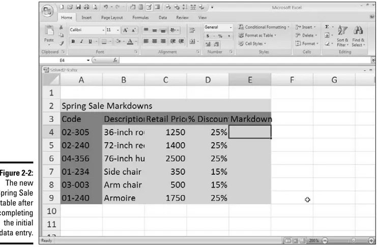
1. Enter the table title Spring Sale Markdowns in cell A2.
2. Enter the column headings in row 3 as follows: •Code in cell A3
•Descriptionin cell B3 •Retail Pricein cell C3 •% Discountin cell D3 •Markdownin cell E3
3. Enter the code numbers in column A as follows (don’t forget how to override Excel and enter these codes as text entries by prefacing each of them with an apostrophe):
•02-305in cell A4 •02-240in cell A5 •04-356in cell A6 •01-234in cell A7 •03-003in cell A8 •01-240in cell A9
4. Enter the furniture descriptions in column B as follows: •36-inch round tablein cell B4
•72-inch rectangle tablein cell B5 •76-inch hutchin cell B6
•Side chairin cell B7 •Arm chairin cell B8 •Armoirein cell B9
5. Enter the retail prices of the furniture in column C as follows: •1250in cell C4
•1400in cell C5 •2500in cell C6 •350in cell C7 •500in cell C8 •1750in cell C9