Fundamentals
of Digital
Image Processing
ANIL K. JAIN University of California, Davis
6.1 INTRODUCTION
6
Image Representation by Stochastic Models
In stochastic representations an image is considered to be a sample function of an array of random variables called a random field (see Section 2.10). This characteri zation of an ensemble of images is useful in developing image processing techniques that are valid for an entire class and not just for an individual image.
Covariance Models
In many applications such as image restoration and data compression it is often sufficient to characterize an ensemble of images by its mean and covariance func tions. Often one starts with a stationary random field representation where the mean is held constant and the covariance function is represented by the separable or the nonseparable exponential models defined in Section 2.10. The separable covar iance model of (2.84) is very convenient for analysis of image processing algorithms, and it also yields computationally attractive algorithms (for example, algorithms that can be implemented line by line and then column by column). On the other hand, the nonseparable covariance function of (2.85) is a better model [21] but is not as convenient for analysis.
Covariance models have been found useful in transform image coding, where the covariance function is used to determine the variances of the transform coeffi cients. Autocorrelation models with spatially varying mean and variance but spa tially invariant correlation have been found useful in adaptive block-by-block pro cessing techniques in image coding and restoration problems.
Linear System Models
An alternative to representing random fields by mean and covariance functions is to characterize them as the outputs of linear systems whose inputs are random fields
Stochastic models used in image processing
Covari a nee models One-dimensional ( 1 -D) models Two-dimensional (2-D) models • Separable exponential
• Nonseparable exponential
· A R and A R M A • State variable • Noncausal minimum
variance
• Causal • Semicausal • Noncausal
Figure 6.1 Stochastic models used in image processing.
with known or desired statistical properties (for example, white noise inputs). Such linear systems are represented by difference equations and are often useful in developing computationally efficient image processing algorithms. Also, adaptive algorithms based on updating the difference equation parameters are easier to implement than those based on updating covariance functions. The problem of finding a linear stochastic difference equation model that realizes the covariances of an ensemble is known as the spectral factorization problem.
Figure 6.1 summarizes the stochastic models that have been used in image processing [1]. Applications of stochastic image models are in image data compres sion, image restoration, texture synthesis and analysis, two-dimensional power spectrum estimation, edge extraction from noisy images, image reconstruction from noisy projections, and in several other situations.
6.2 ONE-DIMENSIONAL ( 1 -D) CAUSAL MODELS
A simple way of characterizing an image is to consider it a 1-D signal that appears at the output of a raster scanner, that is, a sequence of rows or columns. If the interrow or inter-column dependencies are ignored then 1-D linear systems are useful for modeling such signals. Let
u(n) be a real, stationary random sequence with zero mean and covariance r(n). If u(n) is considered as the output of a stable, linear shift invariant system H(z) whose input is a stationary zero mean random sequence e(n), then its SDF is given by
S(z) = H(z)S.(z)H(z -1), (6.1)
where S.(z) is the SDF of e(n). If H(z) must also be causal while remaining stable, then it must have a one-sided Laurent series
H(z) = L h(n)z-n (6.2)
n = O and all its poles must lie inside the unit circle [2]. Autoregressive (AR) Models
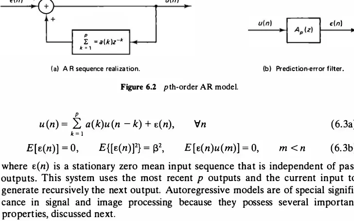
e(n) + u(n)
where E(n) is a stationary zero mean input sequence that is independent of past outputs. This system uses the most recent p outputs and the current input to generate recursively the next output. Autoregressive models are of special signifi cance in signal and image processing because they possess several important properties, discussed next.
is the best linear mean square predictor of u(n) based on all its past but depends only on the previous p samples. For Gaussian sequences this means a pth-order AR sequence is a Markov-p process [see eq. (2.66b)]. Thus (6.3a) can be written as
u(n) = u (n) + E(n) (6.5)
which says the sample at n is the sum of its minimum variance, causal, prediction estimate plus the prediction error E(n), which is also called the innovations sequence. Because of this property an AR model is sometimes called a causal minimum variance representation (MVR). The causal filter defined by
p
Ap (z)
�
1 -
L a (n)z-n (6.6)n = I
is called the prediction error filter. This filter generates the prediction error se quence E(n) from the sequence u(n).
The prediction error sequence is white, that is,
E[E(n)E(m)] = �28(n -m) (6.7)
For this reason, AP (z) is also called the whitening filter for u(n). The proof is considered in Problem 6.1.
Except for possible zeros at z = 0, the transfer function and the SDF of an AR
process are all-pole models. This follows by inspection of the transfer function
where the properties of e(n) are same as before. This representation can also be written as
u(n) =
k
t
a (k)u(n - k) + e(n) + µ[
1 -kt
l a (k)]
(6.lOb)which is equivalent to assuming (6.3a) with E[e(n)] = µ[l - �k a (k)], cov[e(n)e(m)] = 132 8(n - m).
Identification of AR models. Multiplying both sides of (6.3a) by e(m), taking expectations and using (6.3b) and (6.7) we get
E[u(n)e(m)] = E[e(n)e(m)] = j32 8(n - m), m 2! n (6.11) Now, multiplying both sides of (6.3a) by u(O) and taking expectations, we find the AR model satisfies the relation
p
r(n) - 2: a (k)r(n - k) = 132 8(n), Vn � 0 (6.12) k = l
where r(n) � E[u(n)u(O)] is the covariance function of u(n). This result is im portant for identification of the AR model parameters a (k), 132 from a given set of covariances {r(n), -p s n s p }. In fact, a pth-order AR model can be uniquely determined by solving (6.12) for n = 0, . . . ,p. In matrix notation, this is equivalent
and a � [a(l)a (2) . . . a (p)y, r � [r(l)r(2) . . . r(p)y. If R is positive definite, then the AR model is guaranteed to be stable, that is, the solution {a (k), 1 :::::;; k :::::;; p} is such that the roots of AP (z) lie inside the unit circle. This procedure allows us to fit a stable AR model to any sequence u(n) whose p + 1 covariances r(O), r(l), r(2), . . . , r(p) are known.
Example 6.1.
The covariance function of a raster scan line of an image can be obtained by consider ing the covariance between two pixels on the same row. Both the 2-D models of (2.84) and (2.85) reduce to a 1-D model of the form r(n) = a2 p1"1• To fit an AR model of order 2, for instance, we solve
a2
[� i][:g�]
= a2[�2]
which gives a (1) = p, a (2) = 0, and 132 = a2 (1 -p2). The corresponding representation
for a scan line of the image, having pixel mean of µ., is a first-order AR model
x(n) = px(n - 1) + E(n),
u (n) = x (n) + µ. (6.14)
with A (z) = 1 - pz -1, S. = a2 (1 - p2), and S(z) = a2 (1 - p2)/[(1 - pz -1)(1 - pz)]. Maximum entropy extension. Suppose we are given a positive definite sequence r(n) for lnl ::5p (that is, R is a positive definite matrix). Then it is possible to extrapolate r(n) for ln l >p by first fitting an AR model via (6.13a) and (6.13b) and then running the recursions of (6.12) for n > p, that is, by solving
p
r(p + n) = 2: a (k)r(p + n - k),
k � I r(-n) = r(n),
Vn ;::: 1
}
Vn (6.15)
This extension has the property that among all possible positive definite extensions of {r(n)}, for In I > p, it maximizes the entropy
1
f"
H �2'IT _,, logS(w)dw (6.16)
where S(w) is the Fourier transform of {r(n),Vn}. The AR model SDFt S(w), which can be evaluated from the knowledge of a (n) via (6.9), is also called the maximum entropy spectrum of {r (n ), In I :::::;; p}. This result gives a method of estimating the power spectrum of a partially observed signal. One would start with an estimate of the p + 1 covariances, {r(n), 0 :::::;; n :::::;; p }, calculate the AR model parameters �2, a (k), k = 1, . .. ,p, and finally evaluate (6.9). This algorithm is also useful in certain
image restoration problems [see Section 8.14 and Problem 8.26]. Applications of AR Models in Image Processing
As seen from Example 6.1, AR models are useful in image processing for repre senting image scan lines. The prediction property of the AR models has been
t Recall from Section 2.11 our notation S(w) � S (z), z = eiw.
vn (O) En (Q)
Ap, 0 (z) AR model
nth column Unitary Vn (k) En (k) Vn (k) Un
transform Ap, k (z) AR model ,.,-1
Un "'
AP. N -1 (z) AR model
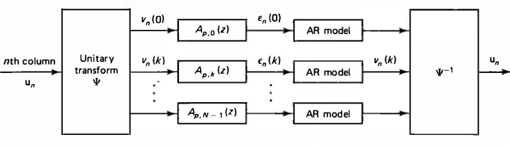
Figure 6.3 Semirecursive representation of images.
exploited in data compression of images and other signals. For example, a digitized AR sequence u (n) reKresented by B bits/sample is completely equivalent to the digital sequence e (n) = u(n) -Il (n), where u:· (n) is the quantized value of u (n). The quantity e (n) represents the unpredictable component of u (n), and its entropy is generally much less than that of u ( n ). Therefore, it can be encoded by many fewer
bits per sample than B. AR models have also been found very useful in representa tion and linear predictive coding (LPC) of speech signals [7].
Another useful application of AR models is in semirecursive representation of images. Each image column Un, n = 0, 1, 2, ... , is first transformed by a unitary
matrix, and each row of the resulting image is represented by an independent AR model. Thus if Vn � Wun, where 'I' is a unitary transform, then the sequence {vn (k), n = 0, 1, 2 .. . } is represented by an AR model for each k (Figure 6.3), as
p
Vn (k) =
i�l
a;(k)vn_; (k) + En (k), 'Tin, k = 0, 1, . . . 'N -1}
E[ En (k)] = 0, E[ En (k)En· (k ')] = 132 (k)8(n - n ')8(k - k ')(6.17) The optimal choice of 'I' is the KL transform of the ensemble of all the image columns so that the elements of vn are uncorrelated. In practice, the value of p = 1 or 2 is sufficient, and fast transforms such as the cosine or the sine transform are good substitutes for the KL transform. In Section 6.9 we will see that certain, so-called semi causal models also yield this type of representation. Such models are useful in filtering and data compression of images [see Sections 8.12 and 11.6]. Moving Average (MA) Representations
A random sequence u (n) is called a moving average (MA) process of order q when
it can be written as a weighted running average of uncorrelated random variables
q
u(n) = L b (k)E(n - k) (6.18)
k=O
where E(n) is a zero mean white noise process of variance 132 (Fig. 6.4). The SDF of this MA is given by
e(n) u{n)
q
r b{k)z-k
q
Bq (z) = L b(k)z -k k=O
(6.19a) (6.19b) From the preceding relations it is easy to deduce that the covariance sequence of a qth-order MA is zero outside the interval [-q, q ]. In general, any covariance sequence that is zero outside the interval [-q, q] can be generated by a qth-order MA filter Bq (z). Note that Bq (z) is an FIR filter, which means MA representations are all-zero models.
Example 6.2
Consider the first-order MA process
u(n) = E(n) - o:E(n - 1), E[E(n)E(m)] = 132 B(m - n)
Then B1 (z) = 1 - o:z -1, S(z) = 132[1 + o:2 - o:(z + z -1)]. This shows the covariance se
quence of u(n) is r(O) = 132 (1 + o:2), r(±l) = -0:132, r(n) = 0, ln l > 1.
Autoregressive Moving Average (ARMA) Representations
An AR model whose input is an MA sequence yields a representation of the type (Fig. 6.5)
p q
L a(k)u(n - k) = L b(l)E(n - l) (6.20)
k=O l=O
where E(n) is a zero mean white sequence of variance 132. This is called an ARMA representation of order (p, q). Its transfer function and the SDF are given by
H(z) = AP (z) Bq (z)
S(z) = 132 AP (z)Ap (z -1) Bq (z)Bq (z -1)
For q = 0, it is a pth-order AR and for p = 0, it is a qth-order MA. State Variable Models
(6.21)
(6.22)
A state variable representation of a random vector sequence Yn is of the form [see
Fig. 8.22(a)]
Vn (6.23)
Here Xn is an m x 1 vector whose elements Xn (i), i = 1, . .. , m are called the states
of the process Yn , which may represent the image pixel at time or location n ; En is a e(n)
Sec. 6.2
1/AP (z) AR model
u(n)
One-dimensional ( 1 -D) Causal Models
Figure 6.5 (p, q)-order ARMA model.
p x 1 vector sequence of independent random variables and Tin is the additive white
noise. The matrices An , Bn , and en are of appropriate dimensions and Tin , En satisfy E[En] = O, E[11n11�·] = Qn 8(n - n '), E[11n] = O
}
(6.24) E[11n E�·] = O, E[En E�·] = Pn S(n - n '), 'Vn, n 'The state variable model just defined is also a vector Markov-1 process. The ARMA models discussed earlier are special cases of state variable models. The application of state variable models in image restoration is discussed in Sections 8.10 and 8.11.
Image Scanning Models
The output s (k) of a raster scanned image becomes a nonstationary sequence even when the image is represented by a stationary random field. This is because equal intervals between scanner outputs do not correspond to equal distances in their spatial locations. [Also see Problem 6.3.] Thus the covariance function
rs (k, I) � E{[s(k) - µ][s(k
-/) -
µ]} (6.25) depends on k, the position of the raster, as well as the displacement variable/.
Such a covariance function can only yield a time-varying realization, which would increase the complexity of associated processing algorithms. A practical alternative is to replace r, (k, I) by its average over the scanner locations [9], that is, byN - 1
rs (l) �
�
k2:/s(k, I) (6.26)Given rs (l), we can find a suitable order AR realization using (6.12) or the results of the following two sections. Another alternative is to determine a so-called cyclo stationary state variable model, which requires a periodic initialization of the states for the scanning process. A vector scanning model, which is Markov and time
invariant, can be obtained from the cyclostationary model [10]. State variable scanning models have also been generalized to two dimensions [11, 12]. The causal models considered in Section 6.6 are examples of these.
6.3 ONE-DIMENSIONAL SPECTRAL FACTORIZATION
Spectral factorization refers to the determination of a white noise driven linear system such that the power spectrum density of its output matches a given SDF. Basically, we have to find a causal and stable filter H(z) whose white noise input has the spectral density K, a constant, such that
S (z) = KH(z)H(z -1), (6.27)
where S(z) is the given SDF. Since, for z = ei"',
S(ei"') � S (w) = K
I
H(w)l
2 (6.28)specifying the phase of
H
( w)
, because its magnitude can be calculated within a constant fromS
( w)
.Rational SDFs
S(z)
is called a proper rational function if it is a ratio of polynomials that can be factored, as in (6.27), such thatH(z) = Bq (z)
Ap(z)
where
AP (z)
andBq (z)
are polynomials of the formp
q
Ap(z) = l -
La(k)z-\
Bq(z)=
L b (k)z-kk = I k = O
(6.29)
(6.30) For such SDFs it is always possible to find a causal and stable filter
H(z).
The method is based on a fundamental result in algebra, which states that any polynomial Pn (x) of degree n has exactly n roots, so that it can be reduced to aproduct of first-order polynomials, that is, n
Pn (x) = TI (a;X -j3;) (6.31) i = l
For a proper rational
S(z),
which is strictly positive and bounded forz =
ei"', there will be no roots (poles or zeros) on the unit circle. SinceS(z) = S(z-1),
for every root inside the unit circle there is a root outside the unit circle. Hence, ifH(z)
is chosen so that it is causal and all the roots ofAP (z)
lie inside the unit circle, then (6.27) will be satisfied, and we will have a causal and stable realization. Moreover, ifBq (z)
is chosen to be causal and such that its roots also lie inside the unit circle, then the inverse filter1/H(z),
which isAP (z)!Bq (z),
is also causal and stable.A
filter that is causal and stable and has a causal, stable inverse is called a minimum-phase filter.Example 6.3
Let
( ) 4.25 - + z s z =
2.5 - (z + z-1) (6.32)
The roots of the numerator are z1 = 0.25 and z2 = 4 and those of the denominator are z3 = 0.5 and z4 = 2. Note the roots occur in reciprocal pairs. Now we can write
( ) -
-s z =
(1 - 0.5z-1)(1 - 0.5z)
Comparing this with (6.32), we obtain K = 2. Hence a filter with H(z) = (1 - 0.25z-1)/
(1 - 0.5z -1) whose input is zero mean white noise with variance of 2, will be a mini mum phase realization of S(z). The representation of this system will be
u(n) = 0.5u(n -1) + e(n) - 0.25e(n - 1)
E[e(n)] = 0, E[e(n)e(m)] = 28(n - m) (6.33)
This is an ARMA model of order (1, 1).
Remarks
It is not possible to find finite-order ARMA realizations when S(z) is not rational. The spectral factors are irrational, that is, they have infinite Laurent series. In practice, suitable approximations are made to obtain finite-order models. There is a subtle difference between the terms realization and modeling that should be pointed out here. Realization refers to an exact matching of the SDF or the covariances of the model output to the given quantities. Modeling refers to an approximation of the realization such that the match is close or as close as we wish. One method of finding minimum phase realizations when S(z) is not rational is by the Wiener-Doob spectral decomposition technique [5, 6]. This is discussed for 2-D case in Section 6.8. The method can be easily adapted to 1-D signals (see Problem 6.6).
6.4 AR MODELS, SPECTRAL FACTORIZATION, AND LEVINSON ALGORITHM
The theory of AR models offers an attractive method of approximating a given SDF arbitrarily closely by a finite order AR spectrum. Specifically, (6.13a) and (6.13b) can be solved for a sufficiently large p such that the SDF SP (z)
�
13�/[AP (z)AP (z-1)] is as close to the given S(z), z = exp(jw), as we wish under some mild restrictions on S(z) [1]. This gives the spectral factorization of S(z) asp - oo. If S(z) happens tohave the rational form of ( 6. 9), then a (n) will turn out to be zero for all n > p. An efficient method of solving (6.13a) and (6.13b) is given by the following algorithm. The Levinson-Durbin Algorithm
This algorithm recursively solves the sequence of problems Rn an = r n
o
r (0) -a� r n = 13�, n = 1, 2, . . . , where n denotes the size of the Toeplitz matrix Rn � {r(i -j), 1 < i, j < n }. The rn and an are n x 1 vectors of elements r(k) and an (k), k = 1, . . . , n. For any Hermitan Toeplitz matrix Rn, the solution at step n is given by the recursions{an- 1 (k) - pna:- 1 (n - k); an (0) = 1, a. (k) = p. ,
13� = 13� - t (1 -Pn P: ), 13� = r(O)
Pn + l =-4-13n
[
r(n + 1) -k = I ± an (k)r(n + 1 - k)]
,l :s k :s n - 1, n ?: 2 k = n, n ?: 1
r(l) Pt = r(O)
(6.34)
The quantities {pn, 1 :5 n :5 p} are called the partial correlations, and their negatives, -pn, are called the reflection coefficients of the pth-order AR model. The quantity Pn represents correlation between u(m) and u(m + n) if u(m + 1), . . . , u(m + n -1) are held fixed. It can be shown that the AR model is stable, that is, the roots of AP (z) are inside the unit circle, if IPn I < l. This condition is satisfied when R is positive definite.
The Levinson recursions give a useful algorithm for determining a finite-order stable AR model whose spectrum fits a given SDF arbitrarily closely (Fig. 6.6). Given r(O) and any one of the sequences {r(n)}, {a(n)}, {pn}, the remaining se quences can be determined uniquely from these recursions. This property is useful in developing the stability tests for 2-D systems. The Levinson algorithm is also useful in modeling 2-D random fields, where the SDFs rarely have rational factors.
Example 6.4
The result of AR modeling problem discussed in Example 6.1 can also be obtained by applying the Levinson recursions for p = 2. Thus r(O) = <T 2, r(l) = <T 2 p, r(2) = <T 2 p2
and we get
1
P2 = l3 � [ <T 2 P2 - P<T 2 P] = 0
This gives 132 = 13� = 13� , a(l) = a2(1) = a1 (1) = p, and a (2) = a2 (2) = 0, which leads to (6.14). Since IPd and IP2I are less than l, this AR model is stable.
S(w)
Sec. 6.4
r ( n) Levinson
recursions
p -+ p + l
No
AP (w) SP (w)
ll;t 1 AP (w) l2
Yes
p
Figure 6.6 AR modeling via Levinson recursions. Ap(w) � 1 - L ap(k) eik� k - 1
6.5 NONCAUSAL REPRESENTATIONS
Causal prediction, as in the case of AR models, is motivated by the fact that a scanning process orders the image pixels in a time sequence. As such, images represent spatial information and have no causality associated in those coordinates. It is, therefore, natural to think of prediction processes that do not impose the causality constraints, that is, noncausal predictors. A linear noncausal predictor
u (n) depends on the past as well as the future values of u (n ). It is of the form
u (n) = L a(k)u(n - k) (6.35)
where a(k) are determined to minimize the variance of the prediction error u (n) -u (n). The noncausal MVR of a random sequence u (n) is then defined as
u (n) = u (n) + v(n) = L a(k)u(n - k) + v(n)
k = - x:
k 4' 0
(6.36)
where v(n) is the noncausal prediction error sequence. Figure 6.7a shows the noncausal MVR system representation. The sequence u(n) is the output of a non causal system whose input is the noncausal prediction error sequence v(n). The transfer function of this system is l/A (z), where A (z) � 1 -2" * O a(n)z-n is called the noncausal MVR prediction error filter. The filter coefficients a(n) can be deter mined according to the following theorem.
Theorem 6.1 (Noncausal MVR theorem). Let u (n) be a zero mean, sta tionary random sequence whose SDF is S(z). If 1/S(ei"') has the Fourier series
� i: r+ (n)e-jwn
S(e1"') n � -"'
then u(n) has the noncausal MVR of (6.36), where -r+ (n)
a(n) = r+ (o) 132 � E{[v(n)]2} =
(6.37)
(6.38)
Moreover, the covariances r. (n) and the SDF S. (z) of the noncausal prediction error v(n) are given by
r. (n) = -131a(n), a(0) � -1
l
S. (z) = 132A (z) � 132[
1-n
�"'
a(n)z-n]
(6.39)v(n) u(n)
A(z) = 1 - L a(n)z-n
n = -cio n ;' Q
(a) Noncausal system representation.
r+ (0) a(n) = -r+ (n)
r+ (0)
(b) Realization of prediction error filter coefficients.
Figure 6.7 Noncausal MVRs. Remarks
1. The noncausal prediction error sequence is not white. This follows from (6.39). Also, since rv (-n) = rv (n), the filter coefficient sequence a(n) is even, that is, a(-n) = a(n), which implies A (z-1) = A (z).
2. For the linear noncausal system of Fig. 6.7a, the output SDF is given by S(z) = Sv (z)/[A (z)A (z-1)]. Using (6.39) and the fact that A (z) = A (z -1), this becomes
_ 132A (z) _ __j£_
S(z) - [A (z)A (z-1)] -A (z) (6.40)
3. Figure 6. 7b shows the algorithm for realization of noncausal MVR filter coefficients. Eq. (6.40) and Fig. 6.7b show spectral factorization of S(z) is not
required for realizing noncausal MVRs. To obtain a finite-order model, the Fourier series coefficients r+ (n) should be truncated to a sufficient number of terms, say, p. Alternatively, we can find the optimum pth-order minimum variance noncausal prediction error filter. For sufficiently large p, these methods yield finite-order, stable, noncausal MVR-models while matching the given covariances to a desired accuracy.
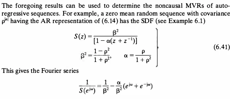
Noncausal MVRs of Autoregressive Sequences
The foregoing results can be used to determine the noncausal MVRs of auto regressive sequences. For example, a zero mean random sequence with covariance plnl having the AR representation of (6.14) has the SDF (see Example 6.1)
S(z) -- [1 - a(z + z-1)]
This gives the Fourier series
1 -p2 - 1 + p2'
Sec. 6.5 Noncausal Representations
p
a =
--1 + p2
(6.41)
which means
a(O) = -1, a(l) = a(-1) = a, r+ (0) = �2 1
The resulting noncausal MVR is
u(n) = a[u(n - 1) + u(n + 1)] + v(n) A (z) = 1 - a(z + z -1)
rv (n) = �2{1 - a[8(n - 1) + 8(n + 1)]}
Sv (z) = �2[1 - a(z + z-1)]
(6.42)
where v(n) is a first-order MA sequence. On the other hand, the AR representation of (6.14) is a causal MVR whose input E(n) is a white noise sequence. The generali zation of (6.42) yields the noncausal MVR of a pth-order AR sequence as
p
u(n) = k= I L a(k)[u(n - k) + u(n + k)] + v(n) p
A (z) = 1 - L a(k)(z-k + zk) k= l (6.43)
Sv (z) = ��A (z)
where v(n) is apth-order MA with zero mean and variance �� (see Problem 6.11).
A Fast KL Transform [13)
The foregoing noncausal MVRs give the following interesting result.
Theorem 6.2. The KL transform of a stationary first-order AR sequence {u (n ), 1 :5 n :5 N} whose boundary variables u (0) and u (N + 1) are known is the sine transform, which is a fast transform.
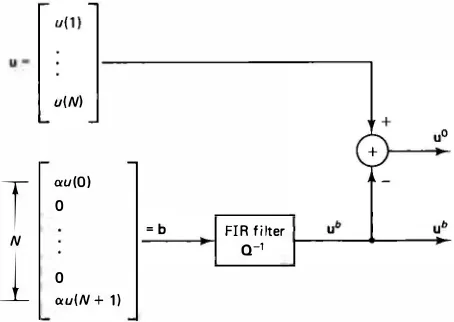
Proof. Writing the noncausal representation of (6.42) in matrix notation,
where u and 11 are N x 1 vectors consisting of elements {u(n), 1 :s; n :s; N} and {v(n), 1 :s; n :s; N}, respectively, we get
Qu = 11 + b (6.44)
where Q is defined in (5 .102) and b contains only the two boundary values, u (0) and u(N + 1). Specifically,
b(l) = au(O), b(N) = au(N + l), b(n) = O, 2 :5 n :5 N - l (6.45) The covariance matrix of 11 is obtained from (6.42), as
Rv � E[1111T] = {rv (m - n)} = �2 Q (6.46)
The orthogonality condition for minimum variance requires that v(n) must be orthogonal to u(k), for all k +. n and E[v(n)u(n)] = E[v2 (n)] = �2• This gives
Multiplying both sides of (6.44) by Q-1 and defining
we obtain an orthogonal decomposition of u as u = u0 + ub
(6.48)
(6.49) Note that ub is orthogonal to u0 due to the orthogonality of v and b [see (6.47)] and
is completely determined by the boundary variables u (O) and u (N + 1). Figure 6.8 shows how this decomposition can be realized. The covariance matrix of u0 is given by
(6.50)
Because 132 is a scalar, the eigenvectors of Ro are the same as those of Q, which we know to be the column vectors of the sine transform (see Section 5.11). Hence, the KL transform of u0 is a fast transform. Moreover, since ub and u0 are orthogonal, the conditional mean of u given u (O), u (N + 1) is simply uh, that is,
f.Lb � E [ulu (O), u (N + 1)] = E [u0 + ublu (O), u (N + 1)]
(6.51)
= E[u0] + E [ublu (O), u (N + 1)] = ub
Therefore,
Cov[ulu (O), u (N + 1)] = E [(u - f.Lb)(u - f.Lbfl = E[u0u071 = Ro (6.52) Hence the KL transform of u conditioned on u (O) and u (N + 1) is the eigenmatrix of R0, that is, the sine transform. In Chapter 11 we use this result for developing a (recursive) block-by-block transform coding algorithm, which is more efficient than the conventional block-by block KL transform coding method. Orthogonal decompositions such as (6.49) can be obtained for higher order AR sequences also (see Problem 6. 12). In general, the KL transform of u0 is determined by the eigenvectors of a banded Toeplitz matrix whose eigenvectors can be approximated by an appropriate transform from the sinusoidal family of orthogonal transforms discussed in Chapter 5.
u(N)
T
N1
cr.u(O)0
0
cr.u(N + 1 )
Sec. 6.5
= b FIR fi lter
a-1
Noncausal Representations
Figure 6.8 Noncausal orthogonal de composition for first-order AR se quences.
Optimum Interpolation of Images
The noncausal MVRs are also useful in finding the optimum interpolators for random sequences. For example, suppose a line of an image, represented by a first-order AR model, is subsampled so that N samples are missing between given samples. Then the best mean square estimate of a missing sample u (n) is u (n) � E[u(n)lu(O), u(N + 1)], which is precisely ub (n), that is,
ii = Q-1 b :? u (n) = a[Q-1]n, 1 u(O) + a[Q-1]n, Nu (N + 1) (6.53) When the interpixel correlation p� 1 , it can be shown that u (n) is the straight-line
interpolator between u(O) and u (N + 1), that is,
u (n) = u(O) N + l + 1) -u(O)] (6.54)
For values of p near 1, the interpolation formula of (6.53) becomes a cubic poly
nomial in nl(N + 1) (Problem 6.13).
6.6 LINEAR PREDICTION IN TWO DIMENSIONS
The notion of causality does not extend naturally to two or higher dimensions. Line-by-line processing techniques that utilize the simple 1-D algorithms do not exploit the 2-D structure and the interline dependence. Since causality has no intrinsic importance in two dimensions, it is natural to consider other data structures to characterize 2-D models. There are three canonical forms, namely, causal, semi causal, and noncausal, that we shall consider here in the framework of linear prediction.
These three types of stochastic models have application in many image process ing problems. For example, causal models yield recursive algorithms in data com pression of images by the differential pulse code modulation (DPCM) technique and in recursive filtering of images.
Semicausal models are causal in one dimension and noncausal in the other and lead themselves naturally to hybrid algorithms, which are recursive in one dimen sion and unitary transform based (nonrecursive) in the other. The unitary transform decorrelates the data in the noncausal dimension, setting up the causal dimension for processing by 1-D techniques. Such techniques combine the advantages of high performance of transform-based methods and ease of implementation of 1-D algorithms.
The linear prediction models considered here can also be used effectively for 2-D spectral factorization and spectral estimation. Details are considered in Section 6.7.
Let u(m, n) be a stationary random field with zero mean and covariance r(k, l ). Let u(m, n) denote a linear prediction estimate of u(m, n), defined as
u(m, n) = 2: 2: a(k, l )u(m - k, n - l )
(k, /) E S, (6.55)
where a (k, l ) are called the predictor coefficients and .t , a subset of the 2-D lattice, is called the prediction region.
The samples included in Sx depend on the type of prediction considered, namely, causal (x = 1), semicausal (x = 2), or noncausal (x = 3). With a hypothet ical scanning mechanism that scans sequentially from top to bottom and left to right, the three prediction regions are defined as follows.
Causal Prediction
A causal predictor is a function of only the elements that arrive before it. Thus the causal prediction region is (Fig. 6.9a)
51 = {l ::::1,'v'k} u {l = o, k :::: 1} (6.56) This definition of causality includes the special case of single-quadrant causal pre dictors.
u (m, n) = 2: 2: a (k, l )u(m - k, n - 1 )
k = O l = O (k, / ) + (0, 0)
(6.57)
This is called a strongly causal predictor. In signal processing literature the term causal is sometimes used for strongly causal models only, and (6.56) is also called the nonsymmetric half-plane (NSHP) model [22].
" s,
(a) Causal
Sec. 6.6
----(b) Semicausal (c) Noncausal
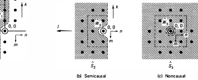
Figure 6.9 Three canonical prediction regions S, and the corresponding finite prediction windows W,, x = 1 , 2, 3.
Semicausal Prediction
A semicausal predictor is causal in one of the coordinates and noncausal in the other. For example, the semicausal prediction region that is causal in n and non causal in m is (Fig. 6.9b)
S2 = {/ 2::1,\fk} u {/ = 0, k 4' O} (6.58)
Noncausal Prediction
A noncausal predictor u(m, n) is a function of possibly all the variables in the random field except u(m, n) itself. The noncausal prediction region is (Fig. 6.9c) S3 = {\f (k, l ) -+ (0, O)} (6.59)
In practice, only a finite neighborhood, called a prediction window, W,, C Sx , can be used in the prediction process, so that
u (m, n) = LL. a (k, l )u (m - k, n - l ),
(k, I) E W,
Some commonly used W,, are (Fig. 6.9)
Causal: Semicausal:
Noncausal:
We also define
Example 6.5
il A
Wt = Wt u (0, 0),
x = l, 2, 3
x = 1, 2, 3
The following are examples of causal, semicausal, and noncausal predictors.
(6.60)
(6.61a)
(6.61b)
Causal: u (m, n) = a1 u(m - l , n) + a2u(m, n - 1) + a3 u(m - l , n - 1) Semicausal: u (m, n) = a1 u(m - l, n) + a2 u(m + l, n) + a3u(m, n - l) Noncausal: u(m, n) = a1 u(m - 1, n) + a2u(m + 1, n) + a3 u(m, n - 1)
+ a4 u(m, n + 1)
Minimum Variance Prediction
Given a prediction region for forming the estimate u (m, n ), the prediction coeffi
cients a (m, n) can be determined using the minimum variance criterion. This re quires that the variance of prediction error be minimized, that is,
�2 � minE[E2(m, n)], E(m, n) � u(m, n) - u(m, n) (6.62) The orthogonality condition associated with this minimum variance prediction is
Using the definitions of E(m, n) and u (m, n ), this yields
The solution of the above simultaneous equations gives the predictor coefficients
a
(i,
j) and the prediction error variance (32• Using the symmetry propertyIn general, the random field u (m, n) can be characterized as
u (m, n) = u (m, n) + E(m, n)
(6.67)
(6.68) where u (m, n) is an arbitrary prediction of u (m, n) and E(m, n) is another random field such that (6.68) realizes the covariance properties of u (m, n). There are three types of representations that are of interest in image processing:
1. Minimum variance representations (MVR) 2. White noise driven representations (WNDR)
3. Autoregressive moving average (ARMA) representations
For minimum variance representations, u (m, n) is chosen to be a minimum variance predictor and E(m, n) is the prediction error. For white noise-driven representa tions E(m, n) is chosen to be a white noise field. In ARMA representations, E(m, n)
is a two-dimensional moving average, that is, a random field with a truncated spectral density function is a (finite-order) two-dimensional polynomial given by
S (zi , z2) = 1 - a(z1 + z;-1 + z2 + z21), lal < �
Finite-Order MVRs
The finite order predictors of (6.60) yield MVRs of the form
u (m, n) = LL a (k, l)u(m - k, n - I) + E(m, n) (6.70)
Ck. I) E w,
A random field characterized by this MVR must satisfy (6.63) and (6.64). Multi plying both sides of (6.70) by E(m, n), taking expectations and using (6.63), we obtain
E[u(m, n)E(m, n)] = 132 Using the preceding results we find
r.(k, I) � E[E(m, n)E(m - k, n - I)]
(6.71)
= E{E(m, n)[u(m - k, n - I) - u(m - k, n - I)]} (6.72) = 132
[
8(k, /) - LL. a (i, j)8(k + i, I + n]
(i, j) E W,
With a(O, 0) � - 1 and using (6.67), the covariance function of the prediction error E(m, n) is obtained as
1328(k, /), \f (k, /) for causal MVRs
p
-132s(t) L a (i, o)s(k + i),
r.(k, I) = i = -p V(k, /) for semicausal MVRs
p q
-132 L L a(i, j)s(k - i)8(1 -n, \f(k, I) for noncausal MVRs
i = -p j = -q
(6.73) The filter represented by the two-dimensional polynomial
A (zi. z2) � 1 - LL. a(m, n)zlm zi" (6.74)
(m,n) E W,
is called the prediction error filter. The prediction error E(m, n) is obtained by passing u(m, n) through this filter. The transfer function of (6.70) is given by
H(zi. z2) = A(Zi, Z2 l ) =
[
1 - LL. a (m, n)zlm z2"(m,n) E W,]
-1 (6.75) Taking the 2-D Z-transform of (6.73) and using (6.74), we obtaincausal MVRs
p
( ) -132 2: a(m, O)zim = 132A (z1>x),
S. Z1> Z2 = m = -p semicausal MVRs
132
[
1 - LL. a (m, n)zlmz2"]
= 132A (z1> z2)(m,n) E W 3 noncausal MVRs
Using (6.75), (6.76) and the symmetry condition A (zi. z2) = A (z)1, z21) for non causal MVRs, we obtain the following expressions for the SDFs:
A (zi. z2)A (z)1, z21) ' f32A (zi. oo)
causal MVRs
semi causal
MVRs (6.77)
non causal MVRs
Thus the SDFs of all MVRs are determined completely by their prediction error filters A (zi. z2) and the prediction error variances 132• From (6.73), we note the causal MVRs are also white noise-driven models, just like the 1-D AR models. The semicausal MVRs are driven by random fields, which are white in the causal dimension and moving averages in the noncausal dimension. The noncausal MVRs are driven by 2-D moving average fields.
Remarks
1. Definition: A two-dimensional sequence x (m, n) is called causal, semicausal,
or noncausal if its region of support is contained in. Si, 52, or 53, respectively. Based on this definition, we call a filter causal, semicausal, or noncausal if its impulse response is causal, semicausal, or noncausal, respectively.
2. If the prediction error filters A (zi. z2) are causal, semicausal, or noncausal, then their inverses l/A (z1, z2) are likewise, respectively.
3. The causal models are recursive, that is, the output sample u (m, n) can be uniquely computed recursively from the past outputs and inputs-from {u(m, n), E(m, n) for (m, n) E S1}. Therefore, causal MVRs are difference equations that can be solved as initial value problems.
The semicausal models are semirecursive, that is, they are recursive only in one dimension. The full vector Un = {u(m, n), 'v'm} can be calculated from the past output vectors {uj,j < n} and all the past and present input vectors
{Ej,j ::::; n }. Therefore, semicausal MVRs are difference equations that have to be solved as initial value problems in one of the dimensions and as boundary value problems in the other dimension.
The noncausal models are nonrecursive because the output u(m, n) depends on all the past and future inputs. Noncausal MVRs are boundary value difference equations.
4. The causal, semicausal, and noncausal models are related to the hyperbolic, parabolic, and elliptic classes, respectively, of partial differential equations [21].
5. Every finite-order causal MVR also has a finite-order noncausal minimum variance representation, although the converse is not true. This is because the SDF of a causal MVR can always be expressed in the form of the SDF of a noncausal MVR.
aS
Figure 6.10 Partition for Markovian ness of random fields.
6. (Markov random fields). A two-dimensional random field is called Markov if at every pixel location we can find a partition J+ (future), aJ (present) and J-(past) of the two-dimensional lattice {m, n} (Fig. 6.10) providing support to the sets of random variables u+' au, and u-' respectively, such that
P[u+1u-, au] = P[u+1au]
This means, given the present (a U), the future ( u+) is independent of the past ( u-). It can be shown that every Gaussian noncausal MVR is a Markov random field [19]. If the noncausal prediction window is [-p, p] x [-q, q], then the random field is called Markov [p x q ]. Using property 5, it can be
shown that every causal MVR is also a Markov random field.
Example 6.7
For the models of Example 6.5, their prediction error filters are given by
A (zi , z2) = l - a1 zl1 - a2z:Z1 - a3z11 z:Z1 (causal model)
A (zi, z2) = 1 - a1 zl1 - a2 z1 - a3 z:Z1 (semicausal model)
A (zi, z2) = l - a1 zl1 - a2 z1 - a3 z21 - a4 Z2 (noncausal model)
Let the prediction error variance be �2• If these are to be MVR filters, then the
following must be true.
Causal model. s. (zi , z2) = �2, which means E(m, n) is a white noise field.
This gives
Su (z1, z2) = (l - a1 z1 - a2 z2 - a3 Z1 z2 -t -1 -1 - a1 z1 - a2 z2 - a3 Z1 Z2 )
Semicausal model. S. (zi , z2) = �2[l - a1 z11 - a2 z1] = �2A (z1, 00). Because
the SDF S. (z1, z2) must equal S. (zl1 , z:Z1), we must have a1 = a2 and
( ) _ �2 (1 - a1 zl1 - a1 z1)
Su Zi, Z2 - -1 -1 -1 ·
(l - a1 z1 - a1 z1 - a3 Z2 )(l - a1 z1 - a1 Z1 - a3z2)
Clearly E(m, n) is a moving average in the m (noncausal) dimension and is white in the n (causal) dimension.
Noncausal model.
s. (z1 , z2) = �2[1 - a1 zl1 - a2 z1 - a3 z21 - a4 z2] = �2 A (z1 , z2)
Now E(m, n) is a two-dimensional moving average field. However, it is a special moving average whose SDF is proportional to the frequency response of the prediction error filter. This allows cancellation of the A (z1, z2) term in the numerator and the denomi nator of the preceding expression for Su (zi. z2).
Example 6.8
Consider the linear system
A (z,, z2) U (zi. z2) = F(z,, z2)
where A (zi. z2) is a causal, semicausal, or noncausal prediction filter discussed in Example 6.7 and F(z1, z2) represents the Z-transform of an arbitrary input f(m, n).
For the causal model, we can write the difference equation
u (m, n) - a1 u (m - l , n) - a2u(m, n -l) - a3 u (m - l, n - 1) = f(m, n)
This equation can be solved recursively for all m � 0, n � 0, for example, if the initial values u(m, 0), u(O, n) and the input f(m, n) are given (see Fig. 6.lla). To obtain the
n - 1 n n - 1 n
n n
•
m - 1 •
m •
m
• •
• •
c 8
D�A
m - 1 • •
f
m • •
m + l • •
• • •
m = N + 1
m
(a) Initial conditions for the causal system. (b) Initial and boundary conditions for the semicausal system.
n -1 n n = N + 1
• • • •
m - 1
+
•m •
m + l • •
m = N + 1
m
(c) Boundary conditions for the noncausal system.
Figure 6.11 Terminal conditions for systems of Example 6.8.
solution at location A, we need only the previously determined solutions at locations
B, C, and D and the input at A. Such problems are called initial-value problems. The semicausal system satisfies the difference equation
u(m, n) - a1 u(m - 1, n) - a2u(m + 1, n) - a3u(m, n - 1) = f(m, n)
Now the solution at (m, n) (see Fig.6.llb) needs the solution at a future location
(m + l, n). However, a unique solution for a column vector Un � [u(l, n), . . . , u(N, n)f can be obtained recursively for all n � 0 if the initial values u (m, 0) and the boundary values u (O, n) and u (N + 1, n) are known and if the coefficients ai, a2, a3
satisfy certain stability conditions discussed shortly. Such problems are called initial boundary-value problems and can be solved semirecursively, that is, recursively in one dimension and nonrecursively in the other.
For the noncausal system, we have
u (m, n) - a1 (m - l,n) - a2u(m + l,n) - a3 (m, n - 1) - a4u(m, n + 1) = f(m, n)
which becomes a boundary-value problem because the solution at (m, n) requires the solutions at (m + l , n) and (m, n + 1) (see Fig. 6.llc).
Note that it is possible to reindex, for example, the semicausal system equation as
1 a1 aJ -1
u (m n) - - u(m - l n) + - u(m - 2 n) + - u(m - l n - l) = -f(m - l n) ' a2 ' a2 ' az ' a2 '
This can seemingly be solved recursively for all m � 0, n � 0 as an initial-value problem if the initial conditions u (m, 0), u (0, n ), u ( -1, n) are known. Similarly, we could re
index the noncausal system equation and write it as an initial-value problem. However, this procedure is nonproductive because semicausal and noncausal systems can become unstable if treated as causal systems and may not yield unique solutions as initial value problems. The stability of these models is considered next.
Stability of Two-Dimensional Systems
In designing image processing techniques, care must be taken to assure the under lying algorithms are stable. The algorithms can be viewed as 2-D systems. These systems should be stable. Otherwise, small errors in calculations (input) can cause large errors in the result (output).
The stability of a linear shift invariant system whose impulse response is h (m, n) requires that (see Section 2.5)
L L lh (m, n)I < 00
m n (6.78)
We define a system to be causal, semicausal, or noncausal if the region of support of its impulse response is contained in Si, S2, or S3, respectively. Based on this
definition, the stability conditions for different models whose transfer function
H(zi, z2) = 1/A (zi, z2), are as follows.
Noncausal systems
q
L a (m, n)zlm zi" (6.79) m = -p n = -q
These are stable as nonrecursive filters if and only if
These are semirecursively stable if and only if
Causal systems
p p q
A (zi,z2) = 1 - L a(m, O)zjm - L L a(m, n)z;-m z2n m = l These are recursively stable if and only if
A (zi, z2) + 0,
These conditions assure H to have a uniformly convergent series in the appro priate regions in the Zi, z2 hyperplane so that (6.78) is satisfied subject to the causality conditions. Proofs are considered in Problem 6.17.
The preceding stability conditions for the causal and semicausal systems require that for each w1 E (- 'TT, 'TT), the one-dimensional prediction error filter A (ei"'1, z2) be stable and causal, that is, all its roots should lie within the unit circle lz21 = 1. This condition can be tested by finding, for each wi, the partial correlations p(w1) associated with A (ei"'1, z2) via the Levinson recursions and verifying that lp(w1)1 < 1 for every w1• For semicausal systems it is also required that the one dimensional polynomial A (zi, oc) be stable as a noncausal prediction error filter,
that is, it should have no zeros on the unit circle. For causal systems, A (zi, oc) should
be stable as a causal prediction error filter, that is, its zeros should be inside the unit circle.
6.7 TWO-DIMENSIONAL SPECTRAL FACTORIZATION
AND SPECTRAL ESTIMATION VIA PREDICTION MODELS
Now we consider the problem of realizing the foregoing three types of representa tions given the spectral density function or, equivalently, the covariance function of the image. Let H(zi, z2) represent the transfer function of a two-dimensional stable linear system. The SDF of the output u(m, n) when forced by a stationary random field E(m, n) is given by
Su (zi, zz) = H(zi, z2)H(z;-1, z21)S. (zi, z2) (6.82)
The problem of finding a stable system H(zi, z2) given Su (zi, z2) and S, (zi, z2) is called the two-dimensional spectral factorization problem. In general, it is not
ble to reduce a two-dimensional polynomial as a product of lower order factors. Thus, unlike in 1-D, it may not be possible to find a suitable finite-order linear system realization of a 2-D rational SDF. To obtain finite-order models our only recourse is to relax the requirement of an exact match of the model SDF with the given SDF. As in the one-dimensional case [see (6.28)] the problem of designing a stable filter H(zi. z2) whose magnitude of the frequency response is given is essentially the same as spectral factorization to obtain white noise-driven representations.
Example 6.9
Consider the SD F
lal < �
Defining A (z2) = 1 - a(z2 + z21), S(zi. z2) can be factored as
S(zi, z2) = A (z2) - a(z1 + z11) = H(zi, z2)H(z11, z21)
where
H(z1, z2) � (l -p(z2)z!1)
�
, p ( ) Z2 = t:.. A (z2) + 2a 2 (z2) -4a2(6.83)
(6.84)
Note that H is not rational. In fact, rational factors satisfying (6.82) are not possible. Therefore, a finite-order linear shift invariant realization of S(z1, z2) is not possible.
Separable Models
If the given SDF is separable, that is, S(zi, z2) = S1 (z1) S2 (z2) or, equivalently, r(k, l) = r1 (k)r2 (l) and S1 (z1) and S2 (z2) have the one-dimensional realizations [H1 (z1), S.Jz1)] and [H2 (z2), S,2 (z2)] [see (6. 1)], then S(zi, z2) has the realization
H(zi, z2) = H1 (zi)H2 (z2)
s. (zi, Z2) = s.1 (z1)S.2 (z2) (6.85) Example 6.10 (Realizations of the separable covariance function)
The separable covariance function of (2.84) can be factored as r1 (k) = CT2 p1�1, r2 (/) =
pl�1• Now the covariance function r(k) � CT 2 p1k1 has (1) a causal first-order AR realiza tion (see Example 6.1) A (z) � 1 - pz - i , S. (z) = CT 2 (1 - p2) and (2) a noncausal MVR
(see Section 6.5) with A (z) � l - a(z + z -1), S. (z) = CT2 132A (z), 132 � (1 - p2)/ (1 + p2), a � p/(l + p2). Applying these results to r1 (k) and r2 (/), we can obtain the following three different realizations, where a,, 13,, i = 1, 2, are defined by replacing p
by p,, i = 1, 2 in the previous definitions of a and 13.
gives Causal MVR (C1 model). Both r1 (k) and rz (/) have causal realizations. This
A (zi, z2) = (1 - P1 Z11)(1 - P2Z21), s. (zi. z2) = CT 2 c1 - Pnc1 - P�)
u(m, n) = p1 u(m - l, n) + p2u(m, n - 1)
- p1 p2u(m - 1, n - l) + E(m, n)
r. (k, l) = a 2 (1 - p�)(l - p�)8(k, l)
Semicausal MVR (SC1 model). Here r1 (k) has noncausal realization, and r2 (l) has causal realization. This yields the semicausal prediction-error filter
A (zi, z2) = [1 - a1 (z1 + z;-1)](1 -Pz z21),
This example shows that all the three canonical forms of minimum variance representa tions are realizable for separable rational SDFs. For nonseparable and/or irrational SDFs, only approximate realizations can be achieved, as explained next.
Realization of Noncausal MVRs
For nonseparable SDFs, the problem of determining the prediction-error filters becomes more difficult. In general, this requires solution of (6.66) with p � oo,
Two-dimensional Spectral Factorization and Spectral Estimation
(6.90)
(6.91)
This is the two-dimensional version of the one-dimensional noncausal MVRs con sidered in Section 6.5.
In general, this representation will be of infinite order unless the Fourier series of 1/S(zi. z2) is finite. An approximate finite-order realization can be obtained by truncating the Fourier series to a finite number of terms such that the truncated series remains positive for every (wi, w2). By keeping the number of terms suf ficiently large, the SDF and the covariances of the finite-order noncausal MVR can be matched arbitrarily closely to the respective given functions [16] .
Example 6.1 1
Realization of Causal and Semicausal MVRs
Inverse Fourier transforming S(eiwi, eiw2) with respect to w1 gives a covariance se quence r1(eiwz), l = integers, which is parametric in w2• Hence for each w2, we can find an AR model realization of order q, for instance, via the Levinson recursion (Section 6.4), which will match r1 (eiw2) for -q :s l :s q.
Let 132 (eiwz), an (eiw2), 1 :s n :s q be the AR model parameters where the predic tion error 132 (eiwz) > 0 for every w2• Now 132 (eiwz) is a one-dimensional SDF and can be factored by one-dimensional spectral factorization techniques. It has been shown that the causal and semicausal MVRs can be realized when 132 (eiwz) is factored by causal (AR) and noncausal MVRs, respectively. To obtain finite-order models an (eiwz) and 132 (eiwz) are replaced by suitable rational approximations of order p, for instance. Stability of the models is ascertained by requiring the reflection coeffi cients associated with the rational approximations of an (eiw2), n = 1, 2, .. . , q to be less than unity in magnitude. The SDFs realized by these finite-order MVRs can be made arbitrarily close to the given SDF by increasing p and q sufficiently. Details
may be found in [16] .
Realization via Orthogonality Condition
The foregoing techniques require working with infinite sets of equations, which have to be truncated in practical situations. A more practical alternative is to start with the covariance sequence r(k, l) and solve the subset of equations (6.66) for (k, l) E Wx C S., that is,
where the dependence of the model parameters on the window size is explicitly shown. These equations are such that the solution for prediction coefficients on W,, requires covariances r(k, /) from a larger window. Consequently, unlike the 1-D AR models, the covariances generated by the model need not match the given covariances used originally to solve for the model coefficients, and there can be many different sets of covariances which yield the same MVR predictors. Also,
stability of the model is not guaranteed for a chosen order.
In spite of the said shortcomings, the advantages of the foregoing method are (1) only a finite number of linear equations need to be solved, and (2) by solving these equations for increasing orders (p, q), it is possible to obtain eventually a finite-order stable model whose covariances match the given r(k, l) to a desired accuracy. Moreover, there is a 2-D Toeplitz structure in (6.93) that can be exploited to compute recursively ap, q (m, n) from aP -l , q (m, n) or ap, q - 1 (m, n ), and so on. This
yields an efficient computational procedure, which is similar to the Levinson Durbin algorithm discussed in Section 6.4.
If the given covariances do indeed come from a finite-order MVR, then the solution of (6.93) would automatically yield that finite-order MVR. Finally, given the solution of (6.93), we can determine the model SDF via (6.77). This feature gives an attractive algorithm for estimating the SDF of a 2-D random field from a limited number of covariances.
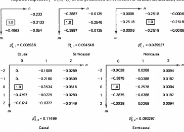
Consider the isotropic covariance function r(k, l) = Figure 6.12 shows the
impulse responses {-a (m, n )} of the prediction error filters for causal, semicausal, and
n origin (0, 0) is at the location of the boxed elements.
n
(a) Given spectrum (b) Semicausal model spectrum Figure 6.13 Spectral match obtained by semicausal MVR of order p = q = 2.
noncausal MVRs of different orders. The difference between the given covariances and those generated by the models has been found to decrease when the model order is increased [16]. Figure 6.13 shows the spectral density match obtained by the semicausal MVR of order (2, 2) is quite good.
Example 6.13 (Two-Dimensional Spectral Estimation)
The spectral estimation problem is to find the SDF estimate of a random field given either a finite number of covariances or a finite number of samples of the random field. As an example, suppose the 2-D covariance sequence
(
k l)
cos 3-rr(k + /)r(k, l) = cos Tr S + 4 + 16 + 0.058(k, l)
is available on a small grid {-16 ::S k, l ::S 16}. These covariances correspond to two
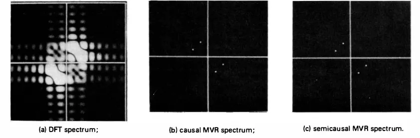
plane waves of small frequency separation in 10-dB noise. The two frequencies are not resolved when the given data is padded with zeros on a 256 x 256 grid and the DIT is taken (Fig. 6.14). The low resolution afforded by Fourier methods can be attributed to the fact that the data are assumed to be zero outside their known extent.
The causal and semicausal models improve the resolution of the SDF estimate beyond the Fourier limit by implicitly providing an extrapolation of the covariance data outside its known extent. The method is to fit a suitable order model that is expected to characterize the underlying random field accurately. To this end, we fit (p, q) = (2, 2)
order models by solving (6.66) for (k, l) E w; where w; C Sx, X = 1, 2 are subsets of
causal and semicausal prediction regions corresponding to (p, q) = (6, 12) and defined
in a similar manner as W,, in (6.61b ). Since Wx C w:, the resulting system of equations is overdetermined and was solved by least squares techniques (see Section 8.9). Note that by solving (6.66) for (k, l) E w:, we are enforcing the orthogonality condition of (6.63) over w:. Ideally, we should let w: = Sx . Practically, a reasonably large region
(a) OFT spectrum ; (b) causal MVR spectrum ; (c) semicausal MVR spectrum.
Figure 6.14 Two-dimensional spectral estimation.
with z1 = exp(jw1), z2 = exp(jw2). Results given in Fig. 6.14 show both the causal and
the semicausal MVRs resolve the two frequencies quite well. This approach has also been employed successfully for spectral estimation when observations of the random field rather than its covariances are available. Details of algorithms for identifying model parameters from such data are given in [17].
6.8 SPECTRAL FACTORIZATION VIA THE WIENER-DOOB HOMOMORPHIC TRANSFORMATION
Another approach to spectral factorization for causal and semicausal models is through the Wiener-Doob homomorphic transformation method. The principle behind this method is to map the poles and zeros of the SDF into singularities of its logarithm. Assume that the SDF S is positive and continuous and the Fourier series of log S is absolutely convergent. Then
m = -:x: n = -'.El
where the cepstrum c(m, n) is absolutely summable
L L ic(m, n)I < 00
m n
Suppose log S is decomposed as a sum of three components log s� s. + c+ +
c-Then
S = A (zi, z2)A - (zi, z2) + s. � s.
H+H-is a product of three factors, where
(6.94)
(6.95)
(6.96)
(6.97)
S • A = exp (s' ) A + • , A = exp -( c+) , A - = exp A ( - - , c ) H + - A +, � -1 H-__a
_l
(6.98) AIf the decomposition is such that A + (zi. z2) equals A - (z11, zi1) and s. (zi. z2) is an SDF, then there exists a stable, two-dimensional linear system with transfer func tion H+ (zi. z2) = l/A + (zi. z2) such that the SDF of the output is S if the SDF of the input is s .. The causal or the semicausal models can be realized by decomposing the cepstrum so that c+ has causal or semicausal regions of support, respectively. The specific decompositions for causal MVRs, semicausal WNDRs, and semicausal MVRs are given next. Figure 6. 15a shows the algorithms.
Causal MVRs [22]
Partition the cepstrum as
c (m, n) = c+ (m, n) + c- (m, n) + .Y. (m, n)
where c+'(m, n) = O, (m, n) ¢ S1; c- (m, n) = O, (m, n) E S1; c+ (O, O) = c- (O, O) = O,
'Y· (m, n) = c (O, 0)8(m, n). S1 and S1 are defined in (6.56) and (6.65), respectively.
Hence we define
"'
c+ = c+ (zi. z2) � L c(m, O)zim + L L c (m, n)zlm Zin
m = l m = -:r:i n = 1
-I "' - l
c-= c-(zi. z2) � L c(m, O)zim + L L C (m, n )zlm Zin m = -:z
A
- A d
s. - s. (zi. z2) = c(O, 0)
m = -o:in = - o:i
(6.99a)
(6.99b)
(6.99c)
Using (6.95) it can be shown that c+ (zi. z2) is analytic in the region {lz11 = 1,
lz21 � 1} U {lz11 � 1, z2 = oo}. Since ex is a monotonic function, A + and H+ are also
analytic in the same region and, therefore, have no singularities in that region. The region of support of their impulse responses a + (m, n) and h + (m, n) will be the same
as that of c+ (m, n), that is, S1 . Hence A + and H+ will be causal filters.
Semicausal WNDRs
Here we let c+ (m, n) = 0, (m, n) $. S2 and define
(6. lOOa)
m = -:r:i m = -:e n = 1
- I
c- (Z1> Z2) = ! L c(m, O)zim+ L L c(m, n)zj'"m zin (6. lOOb)
m = -x m = -:x: n= - :c
(6. lOOc)
,-- -- --- --- --,
(a) Wiener-Doob homomorphic transform method. i/e is the two dimensional homomorphic transform;
-0.0044 0.0023 -0.0016 0.0010
(b) Infinite order prediction error filters obtained by Wiener-Doob factorization for
isotropic covariance model with p = 0.9, a = 1 .
Semicausal MVRs
For semicausal MVRs, it is necessary that s. be proportional to
A+ (zi,oo)
[see(6.76)]. Using this condition we obtain
m = - a:i
m=
-i=D n = 1-1
c-(zi,z2)=
Lc(m, O)zlm+
L Lc(m,n)z1mz2n
m=-m
m = -• n = -•(
6.lOl
a)
(
6.lOl
b)
S,(zi,z2) =
- Lc(m, O)z!m
(6.lOlc)
m = -o:i
The region of analyticity of
c+
andA+
is{lzil = 1,lz21:::::: 1},
and that of s. and s. is{lz11= 1,Vz2}.
Also,a+ (m, n)
and h+ (m, n)
will be semicausal, and s. is a valid SDF. Remarks and Examples1 . For noncausal models, we do not go through this procedure. The Fourier series of
s-1
yields the desired model [see Section 6.7 and (6.91)] .2. Since
c+ (zi, z2)
is analytic, the causal or semicausal filters just obtained are stable and have stable causal or semicausal inverse filters.3. A practical algorithm for implementing this method requires numerical ap proximations via the DFT in the evaluation of S and
A+
or H+.Example 6.14
Consider the SDF of (6.83). Assuming
0 <
o: <O; 1, we obtain the Fourier serieslogS = o:(z1 + z;-1 + z2 + z21) + O (a?). Ignoring O (o:2) terms and using the preceding
results, we get
Causal MVR
� A + (zi , z2) = exp(-C+) = 1 -o:(zl1 + z21), Semicausal MVR
c+ = o:(z1 + z!1) + o:z21, s. = -o:(z1 + z!1)
� A + (zi, z2) = 1 - o:(z1 + z!1) - o:z21 , S. (zi, z2) = 1 -o:(z1 + z!1)
Semicausal WNDR
c+ = 0: ( -1) + -I
Z Z1 + Z1 O:Z2 , s. =
0
Example 6.15
perfect covariance match. Comparing these with Fig. 6.12 we see that the causal and semicausal MVRs of orders (2, 2) are quite close to their infinite-order counterparts in Figure 6.15b.
6.9 IMAGE DECOMPOSITION, FAST KL TRANSFORMS, AND STOCHASTIC DECOUPLING
In Section 6.5 we saw that a one-dimensional noncausal MVR yields an orthogonal decomposition , which leads to the notion of a fast KL transform. These ideas can be generalized to two dimensions by perturbing the boundary conditions of the stochastic image model such that the KL transform of the resulting random field becomes a fast transform. This is useful in developing efficient image processing algorithms. For certain semicausal models this technique yields uncorrelated sets of one-dimensional AR models, which can be processed independently by one dimensional algorithms.
Periodic Random Fields
A convenient representation for images is obtained when the image model is forced
to lie on a doubly periodic grid, that is, a torroid (like a doughnut). In that case, the sequences u (m, n) and E(m, n) are doubly periodic, that is,
E(m, n) = e(m + M, n + N)
u(m, n) = u(m + M, n + N) Vm, n (6.102) where (M, N) are the periods of (m, n) dimensions. For stationary random fields the covariance matrices of u(m, n) and E(m, n) will become doubly block-circulant, and their KL transform will be the two-dimensional unitary DFT, which is a fast transform. The periodic grid assumption is recommended only when the grid size is very large compared to the model order. Periodic models are useful for obtaining asymptotic performance bounds but are quite restrictive in many image processing applications where small (typically 16 x 16) blocks of data are processed at a time. Properties of periodic random field models are discussed in Problem 6.21.
Example 6.16
Suppose the causal MVR of Example 6. 7, written as
u(m, n) = Pi (m -1,
n
) + pz u(m,n
- 1) + p3 u(m - 1, n - 1) + e(m, n) E[e(m, n)] = 0, r. (m, n) = f328(m, n)is defined on an N x N periodic grid. Denoting v (k, I) and e(k, I) as the two
dimensional unitary DFTs of u(m, n) and e(m, n), respectively, we can transform both sides of the model equation as
v(k, I) = (Pi w� + Pz W'N + p3 w� W'N)v (k, I) + e(k, I),
where we have used the fact that u(m, n) is periodic. This can be written as
v (k, I) = e (k, l)IA (k, I), where
A (k, I) = 1 -Pt w� -P2 WN -p3 w� WN
Since e(m, n) is a stationary zero mean sequence uncorrelated over the N x N grid,
e (k, I) is also an uncorrelated sequence with variance p2• This gives
* , , _ E [e (k, l)e* (k 'l')] _ p2 , , E [v (k, l)v (k ' I )] - IA (k, 1)12 - IA(k, 1)12 8(k - k ' l - l )
that is, v (k, I) is an uncorrelated sequence. This means the unitary DFT is the KL transform of u (m, n).
Noncausal Models and Fast KL Transforms
Example 6.17
The noncausal (NC2) model defined by the equation (also see Example 6.7)
u (m, n) - a[u (m - 1, n) + u (m + l , n)
+ u (m, n - 1) + u (m, n + 1)) = e(m, n) (6.103a)
becomes an ARMA representation when
(
e(m, n) is a moving average with covariance 1,r. (k, /) � 132 - 0:1,
0,
(k , l) = (0, 0)
(k , /) = (±1,0) or (0, ± 1) otherwise
For an N x N image U, (6.103a) can be written as QU + UQ = E + B1 + B2
(6.103b)
(6.104)
where b1, b2, b3, and b4 are N x 1 vectors containing the boundary elements of the
image (Fig. 6.16), Q is a symmetric, tridiagonal, Toeplitz matrix with values � along the
I mage U
Boundary values, B
N2 uncorrelated random variables
main diagonal and - a along the two subdiagonals. This random field has the decom
position
U = U° + Ub
where Ub is determined from the boundary values and the KL transform of U0 is the
(fast) sine transform. Specifically,
o _ b
a- - u,- - u,- (6.105)
where a- , a-0, a-b, 6-1 and 6-2 are N2 x 1 vectors obtained by lexicographic ordering of
the N x N matrices U, U0, Ub, B1, and B2, respectively. Figure 6.16 shows a realization of the noncausal model decomposition and the concept of the fast KL transform algo rithm. The appropriate boundary variables of the random field are processed first to obtain the boundary response ub (m, n). Then the residual u0 (m, n) � u(m, n) -ub (m, n) can be processed by its KL transform, which is the (fast) sine transform.
Application of this model in image data compression is discussed in Section 1 1 .5.
Several other low-order noncausal models also yield this type of decomposition [21] .
Semicausal Models and Stochastic Decoupling
Certain semicausal models can be decomposed into a set of uncorrelated one dimensional random sequences (Fig. 6.17). For example, consider the semicausal (SC2) white noise driven representation
u (m, n) - a[u(m - 1 , n) + u (m + 1, n)] = "fU(m, n - 1) + E(m, n) (6. lOQ')
where E(m, n) is a white noise random field with r. (k, I) = 132 B(k, /). For an image with N pixels per column, where Un, En, . . . , represent N x 1 vectors, (6. 106) can be written as
n ;::: 1 (6. 107)
where Q is defined in (5. 102). The N x 1 vector bn contains only two boundary
Sec. 6.9
Boundary values
I nitial values
Figure 6 . 17 Semicausal model decomposition.
N uncorrelated AR processes
terms, bn (1) = au(O, n), bn (N) = au(N + 1, n), bn (m) = 0, 2 � m � N - 1. Now Un can be decomposed as
Un = u� + u� (6. 108)
where
Qu� = "'{U�-1 + bn. ug = Uo (6. 109)
Qu� = "'{U�-1 + En, u8 = 0 (6. 110)
Clearly, u� is a vector sequence generated by the boundary values bn and the initial vector u0 . Multiplying both sides of (6. 110) by 'It, the sine transform, and remem bering that qrrqr = I, 'ltQ'ltT = A = Diag{A(k)}, we obtain
'ltu8 = 0 � Av� = "Yv� - 1 + en (6.1 1 1) where v� and en are the sine transforms of u� and En, respectively. This reduces to a set of equations decoupled in k,
A(k)v� (k) = "'{V� -I (k) + en (k), v8 (k) = 0, n :::::1 , l � k � N
where
(6. 112)
Since En is a stationary white noise vector sequence, its transform coefficients en (k) are uncorrelated in the k-dimension. Therefore, v� (k) are also uncorrelated in the k-dimension and (6. 112) is a set of uncorrelated AR sequences. The semicausal model of (6.87) also yields this type of decomposition [21]. Figure 6.17 shows the realization of semicausal model decompositions. Disregarding the boundary effects, (6. 112) suggests that the rows of a column-by-column transformed image using a suitable unitary transform may be represented by AR models, as mentioned in Section 6.2. This is indeed a useful image representation, and techniques based on such models lead to what are called hybrid algorithms [1, 23, 24], that is, algorithms that are recursive in one dimension and unitary transform based in the other. Applications of semicausal models have been found in image coding, restora tion, edge extraction, and high-resolution spectral estimation in two dimensions.
6.10 SUMMARY