JEJAK
Journal of Economics and Policy http://journal.unnes.ac.id/nju/index.php/jejak
Cointegration and Causality Test Among Export, Import,
and Foreign Exchange
Haryono Subiyakto1 , Algifari2
1STIE YKPN Yogyakarta
Permalink/DOI:http://dx.doi.org/10.15294/jejak.v9i1.7188
Received: January 2016; Accepted: February 2016; Published: March 2016
Abstract
The rupiah exchange rate, import, and export are the important indicators in economy, including the Indonesia economy. The debate regarding the relationship among the exchange rate, import, and export has been persisting for several decades. Some researchers found that there is a relationship among those three and others explained that there is no correlation among them. The aim of this research is to obtain the empirical evidence of the causal relationship among the export, import, and foreign exchange rate by using the monthly data from January 2010 to April 2014. The export and import data are the export and import values in US dollar. The exchange rate data is the median exchange rates of the Indonesian Bank. The Johansen Cointegration Test and the Granger Causality Test are used to analyze the data. The research result shows that export and import have no causal relationship at five percent. Next, the foreign exchange rate influences the export and import at 10 percent level. The result indicates that the foreign exchange rate has small effects on the export and import. Based on the results, the government should control the balance of trade and should not make any policy that is based on the exchange rate values. Finally, it can be said that the exchange rate policy is not effective in increasing the exports and reducing the imports.
Keywords: Exports, Imports, Foreign Exchange Rate, Johansen Cointegration Tests, Granger Causality Tests.
How to Cite: Subiyakto, H., & Algifari, A. (2016). Cointegration and Causality Test Among Export, Import, and Foreign Exchange. JEJAK: Jurnal Ekonomi Dan Kebijakan, 9(1), 82-96. doi:http://dx.doi.org/10.15294/jejak.v9i1.7188
© 2016 Semarang State University. All rights reserved
Corresponding author : ISSN 1979-715X
Address: Jl. Seturan Raya, Caturtunggal,
INTRODUCTION
Foreign exchange rate is the value of domestic currency against the foreign-exchange value. For example, the rupiah exchange against the US dollar is Rp 13,850 / dollar. It means that each dollar of America is worth of Rp 13,850. The foreign exchange rates are always changing in a relatively short time, such as daily time. Everyday the central bank of a country provides the information to the society about the foreign exchange rate in effect on that day. The information on foreign exchange rate is normally used by the society for various purposes, including the export and import activities.
The stable rupiah exchange rate is very important for the economy of Indonesia. In 1997/1998, the time of crisis that was ever experienced by Indonesia led to the depreciation of the rupiah exchange rate, which reached Rp 14,900 per US dollar. The rupiah depreciation has made the entre-preneurs have difficulty in meeting the overseas obligations at the due date and to import the raw materials they need (Harahap, 2013). One of the factors that affects the exchange rate is the availability of foreign currency (foreign exchange reserves) held by Indonesia. The more foreign currency owned by Indonesia will result in the increased value of the rupiah against the foreign-exchange (rupiah is strengthened). This condition is called appreciated rupiah. On the contrary, if the foreign reserve owned by Indonesia is reduced, the value of the rupiah against the foreign-exchange will decrease (the depreciated rupiah).
The increase in Indonesian exports has a very important significance for the economy of Indonesia. Besides being able to stimulate the national production, the increase in
exports could increase the employment and the foreign-exchange revenues, mainly the US dollar. The increased revenue dollars to the Indonesian economy will increase the Indonesian foreign exchange reserves and will give impact on the strengthening of the rupiah against the US dollar.
The industry in Indonesia still requires the raw materials and auxiliary materials that come from abroad (imports). As long as the international transactions are still using the US dollar, the Indonesian import is strongly influenced by the exchange rate of rupiah against the US dollar. If the exchange rate of the rupiah against the US dollar decreases (the rupiah is strengthened), the prices of goods and services from abroad will become relatively cheaper. This will encourage the increase in Indonesianimports. On the contrary, if the rupiah against the US dollar increases (rupiah is weakened), the prices of goods and services coming from abroad will become relatively more expensive and the imports will decrease.
The above description illustrates the causal relationships (influences) among the exports, the imports, and the rupiah exchange rate against the US dollar in Indonesia. Some researches on the causal relationship among the exchange rate, the exports and the imports have been conducted. Alam (2010) conducted a research on the relationship between the changes in the exchange rate against the export revenues in Bangladesh using the annual data from 1977 to 2005 using the cointegration model and the Granger Causality Test. The research has found an empirical evidence of the relationship between the changes in the exchange rates and the export revenues in Bangladesh. A research conducted by Al-Khulaifi (2013) about the relationship of exports and imports in the economy of Qatar using the annual data from 1980 to 2011 found an empirical evidence of the long-term relationship between exports and imports in the economy of Qatar. Khan, et al. (2012) conducted a research on the relationship between the exchange rate and the international trade of the Pakistan economy using the annual data from 1980 to 2009. The research result shows that there is a long-term relationship between the exchange rate and international trade of Pakistan. However, a research of Oyovwi (2012) about the relationship between the exchange change and the imports in the Nigerian economy found no empirical evidence of the influence of the exchange rate against the imports in the Nigerian economy.
Hakim (2012) examined the relationship among the export, the import, and the Gross Domestic Product (GDP) of the Financial Sector of Indonesian Banking using the data from the first Quartal (Q1) in 2000 to the
the previous research conducted by Sekmen and Saribar (2007) using the data from 1998-2006 failed to find the empirical evidence of the influence of foreign exchange rates on the exports and imports in the Turkish economy.
Celik (2012) conducted a research on the long-term relationship between the exports and imports in the Turkish economy using the monthly data from 1990 to 2010. The research found an evidence empirical about the long-term relationship between the exports and imports. The research result of Uddin (2009) on the economy o Bangladesh using the Johansen Cointegration test found an empirical evidence of the two-way mutual relationship in the long term and there is a direct mutual relationship in the short term between the exports and imports. The result of this research is similar to the other research conducted by Mukhtar and Rasheed (2010) on the economy of Pakistan, which managed to find an empirical evidence of the two-way relationship between the exports and imports. However, a researchof Konya and Singh (2008) on the Indian economy found no empirical evidence about the relationship between the exports and imports. Hakim (2011) conducted a research of the existence of cointegration between the exports and imports in the economy of Malaysia and Indonesia using the data for 45 years before and after the economic crisis in Asia. The research managed to obtain an empirical evidence of the long-term relation-ship between the exports and imports in the Malaysian economy. However, there is no long-term relationship between the exports and imports in the Indonesian economy.
RESEARCH METHODS
This research aims to examine the causal relationship among the exports, the imports,
and the exchange rate of rupiah against the dollar of America in Indonesia. Export is the activity of issuing the goods / services from the customs area according to the rules and regulations in force. Customs area is the entire national territory of a country, in which the import and export duties are collected for all the goods that pass through the borderline of the region, except for certain parts in the region that explicitly (by law) are declared as a territory out of the customs. Import is the contrary of the export. The import of a country is an export of the trading partner countries. Imports can be meant as admitting the goods from abroad in accordance with the provisions of the government thah are paid using the foreign exchange. Foreign exchange rate is the value of the domestic currency against the foreign-exchange value (Purnamawati and Fatmawati, 2013).
A country decides to trade with other countries because it aims to gain the benefit from the international trade (gain from trade). Countries that have a superior advantage over the certain goods will export (sell) the goods to other countries that do not have a comparative advantage (Setyowati, 2012). In the international trade, each transaction conducted by a country is assessed in US dollars. Similarly, the exports and imports of Indonesia are assessed with the American dollar, so the value of the American dollar in rupiah (exchange) is critical to the exports and imports of Indonesia.
rupiah against the US dollar makes the price of goods and services in Indonesia assessed by the US dollar decrease. On the contrary, if the rupiah exchange rate against the US dollar decreases (the rupiah is strengthened), the Indonesian exports will decrease, because the strengthening of the rupiah against the US dollar makes the price of goods and services of Indonesia assessed by the American dollar increase.
The data used to examine the causal relationship among the exports, the imports, and the foreign exchange rate in Indonesia isas follows: the value of exports is in US dollars, the value of imports is in US dollars, and the foreign exchange rate is the exchange rate of the rupiah against the US dollar monthly,from Januari 2010 to April 2014. The data on the values of exports, imports, and the exchange rate of rupiah against the US dollar are gained from the website of Bank Indonesia. The model used in this research is a model of Vector Autoregressive (VAR). In the VAR model, all the observed variables are independent and each variable is an endogenous variable. The general model VAR is as follows:
Yt = + 1Yt-1 + 2Yt-2+ …
+ pYt-p + t (1)
Yt is the n x1 matrix of the endogenous
variables in the VAR model, is the m x1 matrix of the exogenous variables, i is the
estimated coefficient matrix, and t is the n x1
matrix of the error terms.
VAR model requires that the data is stationary (Gujarati, 2009). The tests on the data stationary use the Augmented Dickey-Fuller (ADF Test). The general formulation of ADF Test is as follows:
∆Yt = β1+ β2t + δYt-1 +∑mi=1αiYt-i + εt (2)
Yt is the observed variables in period t,
Yt-1 is the variable value of Y in the previous
period. 1 is a constant, 2 is the coefficient of
the trend, i is the lag variable coefficient of
Y, m is the length of lag, and t is the white
noise error terms. The null hypothesis states that = 0. This means that Yt has a unit
roots. If the data of a variable has unit roots, it can be concluded that the variable data is not stationary. If the research data is not stationary at level, the stationary test is continued on the first difference. The stationary research data at different levels need to be examined by the cointegration test. Cointegration is a combination of a linear relationship of the non-stationary variables and all variables must be integrated on the same degree. The integrated variables have the same stochastic trend and the same direction of movement in the long term (Enders, 2004).
The cointegration relationship test among the variables of research conducted uses the Johansen's Multivariate Cointe-gration Test. The general model of the Johansen’s Multivariate Cointegration Test is as follows: Zt = A1 Zt-1 + ... + Ak Zt-k+ Φ Dt +
μ + εt. A1 is the n x n matrix coefficient, μ is a
constant, Dt is the seasonal dummy variable
that is orthogonal to the constant μ and εt is
Ratio). In Ender (2004) it is described the criteria of optimal inaction (lag) of the VAR or VAC models indicated by the smallest value of AIC, SIC, or LR.
While the VAR system stability test is conducted by creating AR Roots Table and Modulus. The VAR system stability can be known from the value of inverse roots of the polynominal function characteristic as follows: Det (1 - A1Z - A2Z2 - A3Z3- ... - ApZp),
where 1 is the identity matrix with the order M x M. If all the roots of the polynomial function are in the unit cyrcle or all modulus are located under one, then the VAR system is called stable. The VAR estimation model needs to test the stability of the VAR estimation equation. The unstable VAR estimation equation makes the analysis of impulse response functions and the analyss of variance decomposition invalid. The test on the VAR estimation equation is conducted.
The next steps are the Analysis of Impulse Response Function and the Analysis of Variance Decomposition. The Analysis of Impulse Response Function (IRF) is conducted to determine the direction of relationships and the influence of an endogenous variable on various endogenous variables in the VAR dynamic system. By using the IRF it can find the effect of the shockthat occurs in one of the endogenous variables to other endogenous ones. IRF also be used to explore the effect of one deviation standard of shock on an endogenous variable to the value of endogenous variable currently or in the future. A shock from an endo-genous variable can be caused by the new information entering at that time and will directly give influence on the endogenous variable itself and also against other endo-genous variables through the VARdynamic
structure. This analysis will know the forms of response (positive or negative) of a varia-ble to the other ones.
This research uses three variables: the export, the import, and the foreign exchange rate. Based on the general form of the VAR model, this research uses of the VAR model as follows:
EXPORTt = 10 +11(L) EXPORT +12(L)IMPORTt +
13(L)EXCHANGE RATEt + 1t
IMPORTt = 20 + 21(L) EXPORT + 22(L)IMPORTt
+ 23(L)EXCHANGE RATEt + 2t
EXCHANGE RATEt = 10 + 11(L) EXPORT +
12(L)IMPORTt + 13(L)EXCHANGE RATEt +
1t
EXPORT is an export, IMPORT is an import, and the EXCHANGE RATE is the rupiah exchange rate against the US dollar, L is the lag, is the error, and t is the period.
RESULTS AND DISCUSSION
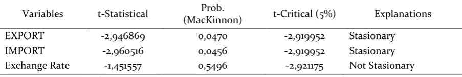
The use of the VAR model requires the data analyzed to be stationary. Table 1 presents the statistical value and the conclusion of the data stationary test result of the export, the import, and the exchange rate by the Augmented Dickey-Fuller test at the level.
The t statistical values for the data stationary test of the export and import are larger than the absolute t critical value at the significance level of 5%. The absolute t statistical value of the export data is 2.946869 and of the import data is 2.960516. The absolute t critical value at the 5%
significance level is 2.919952. The result of the Augmented Dickey-Fuller test shows that the null hypothesis stating that the export data and the import data have unit roots is rejected. The test result shows that export data and the import data are also stationary at the level. The MacKinnon probability value is smaller than the 5% significance level, which indicates that the export data and the import data are stationary at the level. While the absolute t statisticalvalue of the Augmented Dickey-Fuller test for the exchange rate data is 1.451557 smaller than the absolute t critical value of 2.921175. These test results indicate that the exchange rate data has the roots units. In other words, the exchange rate data is not stationary at the level. For the exchange data stationary test it is continued at the level of the first difference. Table 2 below shows the result of the exchange rate data stationary test with the Augmented Dickey-Fuller test at the level of the first difference.
The absolute t statistical value of the exhange rate data is 5.077554, while the absolute t critical at significance level of 5% is 2.922449. The results of the Augmented Dickey-Fuller test indicates that the null hypothesis stating that the exhange rate data of the imports has the roots units is rejected. The test results indicate that the exchange rate data is stationary at the first difference.
Table 1. Data Stationary Test of Export, Import, and Exhange Rate at Level
Variables t-Statistical Prob.
(MacKinnon) t-Critical (5%) Explanations
EXPORT -2,946869 0,0470 -2,919952 Stasionary
IMPORT -2,960516 0,0456 -2,919952 Stasionary
Exchange Rate -1,451557 0,5496 -2,921175 Not Stasionary
Table 2. Exchange Rate Stationary Test at First Difference
Variables t-Statistical Prob.
(MacKinnon) t-Critical (5%) Explanation
Exchange Rate -5,077554 0,0001 -2,922449 Stasionary
Source: Data processed.
The results of the Augmented Dickey-Fuller test show that the exports and imports are stationary at the level, while the exchange rate is stationary at the first difference. The research data that are not stationary at the same level need to take the cointegration test. Table 3 below illustrates the results of the cointegration test using the Johansen Cointegration Test.
The cointegration test results using the Johansen Cointegration Test conclude that there is no cointegration among the variables of the research. The estimation model that
will be used to test the causal relationship among the exports, the imports, and the exchange rate in this research uses the VAR model.
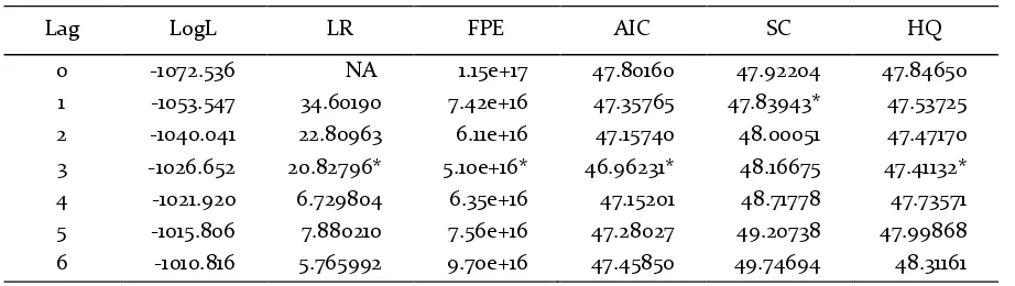
Before determining the estimation equations, it needs to make an analysis of the optimal inaction (lag) of the VAR model among the exports, the imports, andthe foreign exchange rate in this research. Table 4 in the following is the result of data processing to obtain the value of AIC (Akaike Information Criterion), SIC (Schwarz Infor-mation Criterion) and LR (Likelihood Ratio).
Table 3. Johansen Cointegration among Export, Import, and Exchange Rate
H0 H1 Statistical Value Critical Value
(5%) Probability
Trace Statistics
r = 0 r = 1 27,09131 29,79707 0,0994
r =1 r = 2 10,13686 15,49471 0,2704
Maximum Eigenvalue Statistics
r = 0 r >0 16,95445 21,13162 0,1742
r ≤ 0 r > 0 9,336740 14,26460 0,2592 The trace test indicates no cointegration at the 0.05 level
The Max-eigenvalue test indicates no cointegration at the 0.05 level Source: Data processed
Table 4. Inaction (Lag) Order of VAR Model
Lag LogL LR FPE AIC SC HQ
0 -1072.536 NA 1.15e+17 47.80160 47.92204 47.84650
1 -1053.547 34.60190 7.42e+16 47.35765 47.83943* 47.53725 2 -1040.041 22.80963 6.11e+16 47.15740 48.00051 47.47170 3 -1026.652 20.82796* 5.10e+16* 46.96231* 48.16675 47.41132* 4 -1021.920 6.729804 6.35e+16 47.15201 48.71778 47.73571 5 -1015.806 7.880210 7.56e+16 47.28027 49.20738 47.99868 6 -1010.816 5.765992 9.70e+16 47.45850 49.74694 48.31161 * indicates lag order selected by the criterion
The result of the data processing indicates that the optimal inaction (lag) is 3. This is indicated by the most * signs of the calculation results is seen in inaction (lag) 3. Thus the VAR model used to analyze the causal relationship among the exports, the imports, and the rupiah exchange rate against the US dollar is the VAR model with the inaction 3.
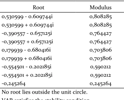
The VAR system stability test is conducted using the root values and the modulus values in The AR Roots Table and the Modulus. The stable VAR system is indicated by the absolute root value that is smaller than the modulus value, and the modulus value that is smaller than 1. Table 5 below VAR shows the results of the VAR system stability test using the root values and the modulus value at the VAR equation with the inaction (lag) 3.
Table 5. Root Values and VAR Modulus Value at Inaction 3
Root Modulus
0,530599 - 0.609744i 0,808285
0,530599 + 0.609744i 0,808285
-0,390557 - 0.657125i 0,764427 -0,390557 + 0.657125i 0,764427
0,179939 - 0.680416i 0,703806
0,179939 + 0.680416i 0,703806
-0,554501 - 0.202185i 0,590212 -0,554501 + 0.202185i 0,590212
-0,245264 0,245264
No root lies outside the unit circle. VAR satisfies the stability condition.
Source: Results of data processing by EViews
The calculation results of the data in Table 5 for the VAR equation with the inaction 3 indicate that the absolute root value is smaller than the modulus value, and the modulus value is smaller than 1. These
results show that the research data is stable at theinaction.
The analysis of the Impulse Response Function is conducted to determine the effects of disturbance (shock) of a variable against the variable itself and against the other variables. Figure 1 in the appendix shows the response of the exports to the shock by one standard deviation that occurs on the export itself, on the imports, and on the exchange rate. The export responds to the shock on itself by fluctuating. In the first and second months the response of the exports is negative and in the significant third month the response is positive, then in the fourth month the response is negative agaian, it is positive at the fifth and sixth months, but the response starts weakening. The export value begins to be stable in the seventh month.
The shock on the imports is responded negatively and positively by the exports, but great. The exports will be stable from the sixth month. While the export response to the changes in exchange rate in the early month is large enough, but the response of the exports runs long enough. That means, if there is a change in the exchange rate, the exports will be stable again and require a relatively long time. The exports will be stable as a result of the changes in the exchange rate in the 11th month.
responded fluctuatively by the import itself and will be stable after the seventh month. The exchange rate response to the changes in the imports is long enough until the exchange rate is stable in the eleventh month.
The exchange rate responds up and down due to the shock on the exports by one standard of deviation. The exchange rate responds positively until the third month and responds negatively in the fourth month, after that it fluctuates until the eleventh month. After the eleventh month, the exchange rate begins to be stable. The response of the exhange rate to the changes in the exchange rate of one standard of deviation is enough up to the fifth month and the fluctuation is weakening after the fifth month. The exchange rate begins to be stable in the thirteenth month. The exchange rate responds to the changes in the exchange rate of one standard of deviation with very large fluctuations. The exchange rate will respond negatively very large up to the fifth month. After the fifth month, it rises up to the eigth month and then falls back after the eight month. The exchange rate will be stable again after the seventeenth month.
The analysis of variance decomposition aims to determine the amounts of portion and the time interval of the influence of the shock on a variable against the variable itself and against other variables. Table 1 and Figure 2 in the Appendix show the amounts of the portion and the time interval of the influence of the changes in the exports, the imports, and the exchange rate towards thechanges in the exports, the imports, and the exchange rate. The calculation results show that in the first month the changes in the export is100% a portion of the change in the export itself and there is no portion of
the change in the import and the exchange rate. In the second month the change in the export is caused by 92.8% from the change in the export itself, 0.5% from the change in the import, and 6.7% came from the change in the exchange rate. The portion of influence of the changes in the export, the import, and the exchange rate towards the change in the export is constant from the seventh month, respectively 89% from the change in the export itself, 3% from the change in the import, and 8% from the change in the exchange rate.
The change in the import in the first month mostly is from the change in the export and in the import itself. While the change in the exchange rate gives no portion to the change in the import. In the first month, the change in the export has a portion of 53% and in the import itself it has 47% of the change in the import. The portion of the changes in the export, the import, and the exchange rate is constant from the tenth month, which is 47% from the change in the export, 41% from the change in the import, and 12% from the change in the exchange rate.
change in the export, 10% from the change in the import, and 83% from the change in the exchange rate itself.
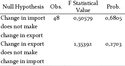
The results of the Granger causality test among the changes in the export, the import, and the exchange rate with the inaction 3 are presented in Table 6, Table 7 and Table 8. Table 6 shows the results of the Granger causality test between the changes in the export and in the import.
Table 6. Granger Causality Test between Changes in Export and in Import
Null Hypothesis Obs. F Statistical
Value Prob. Change in import
does not make change in export
48 0,50579 0,6805
Change in export does not make change in import
1,35392 0,2703
Source: Data processed
The hypothesis testing of the influence of the change in the import towards the change in the export withthe Granger causality test formulates the null hypothesis stating that the change in the import does not make the change in the export. While the alternative hypothesis states the the change in the import makes the change in the export. The F statistical value for the causality test of the changes in the import towards the change in the export is 0.50579 with a probability value of 0.6805. The hypothesis testing of the influence of the change in the export towards the change in the import formulates the null hypothesis that the change in the export does not make the change in the import. The alternate hypothesis states that the change in the export makes the change in the import. The F statistical value for the causality test of the change in the import towards the change in
the export is 1.35392 with a probability value of 0.2703.
The calcultion results of the Granger causality test between the changes in exchange rate and in the export with the inaction 3 are presented in Table 7.
Table 7. Granger Causality Test between Changes in Exchange Rate and in Export
Null Hypothesis Obs. F Statistical
Value Prob. Change in
exchange rate does not make change in export
48 2,77408 0.0543
Change in export does not make change in exchange rate
2,07115 0,1189
Source: Data processed
the exchange rate is 2.07115 with a probability value of 0.1189.
Table 8 presents the calculation results of the Granger causality test between the changes in the exchange rate and in the import with the inaction 3.
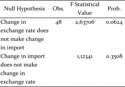
Table 8. Granger Causality Test between Changes in Exchange Rate and in Import
Null Hypothesis Obs. F Statistical
Value Prob. Change in
exchange rate does not make change in import
48 2,63706 0.0624
Change in import does not make change in exchange rate
1,12341 0.3508
Source: Data processed
The hypothesis testing of the influence the change in the exchange rate towards the change in the import by the Granger causality test formulates the null hypothesis stating that the change in the exchange rate does not make the change in the import, and the alternative hypothesis stating that the change in the exchange rates makes the change in the import. The F statistical value for the Granger causality test of th change in the exchange rate towards the change in the import is 2.63706 with a probability value of 0.0624. The hypothesis testing of the influence of the change in the import towards the change in the exchange rate formulates the null hypothesis stating that the change in the import do not make the change in the exchange rate, and the alternative hypothesis states that the change in the import makes the change in the exchange rate. The F statistical value for the causality test of the change in the import
towards the change in the exchange rate is 1.12341 with the probabillity value 0f 0.3508.
This research aims to examine the causal relationship among the exports, the imports, and the exchange rate using the Granger causality test. The testing on the data stationary of the export, the import, and and the exchange rate uses the Augmented Dikkey-Fuller Tests. The testing results of the data stationary indicate that the export data and import data are stationary at the level, while the data of the exchange rate is stationary at the level of the first difference. The results of the Joahnsen cointegration test show that the data of the export, the import, and the exchange rate have no cointegration relationship, so that the estimation of the VAR model uses the data of difference.
The analysis result shows the level of optimal inaction (lag) of the VAR estimation model is at the inaction 3. The stability test result of the VAR estimation model with the inaction 3 using the AR root and modulus table shows that the VAR estimation model with the inaction 3 is stable. The stable VARsystem is shown by the smaller root absolute value than the modulus value, and the modulus value is smaller than 1. Thus, the VAR estimation model at the inaction 3 is valid.
testing receives the null hypothesis stating that the change in the import does not make the change in the export.
The results of the Granger causality test of the change in the exchange rate towards the change in the export show that the F statistical value is 2.77408 with a probability value of 0.0543. With a significance level of 5%, the testingreceives the null hypothesis stating that the change in the exchange rate does not make the changein the export. However, at a significance level of 10%, this testing rejects the null hypothesis. That means, the change in the exchange rates makes the change in the export at a significance level of 10%. The hypothesis testing of the influence of the change in the export towards the change in the exchange rate shows that the F statistical value is 2.07115 with a probability value of 0.1189. With a significance level of 5%, the testing receives the null hypothesis stating that the change in the export does not make the change in the exchange rate.
The results of the Granger causality test of the change in the exchange rate towards the change in in the import obtain the F statistical value as 2.63706 with a probability value of 0.0624. With a significance level of 5%, the testing receives the null hypothesis stating that the change in the exchange rate do not make the change in the import. But at the significance level of10%, the testing rejects the null hypothesis. That means, the change in the exchange rate makes the change in the import at a significance level of 10%. The hypothesis testing of the influence of the change in the import towards the change in the exchange rate with the Granger causality test obtains the F statistic as 1.12341 with a probability value of 0.3508. With a significance level of 5%, the testing
receives the null hypothesis that the change in the import do not make the change in the exchange rate.
CONCLUSION
REFERENCES
Alam, Rafayet (2010). The Link between Real Exchange Rate and Export Earning: A Cointegration and Granger Causality Analysis on Bangladesh. International Review of Business Research Papers Vol.6, No.1. pp.205-214.
Al-Khulaifi, Abdulla S. (2013).Exports and Imports in Qatar: Evidence from Cointegration and Error Correction Model. Asian Economic and Financial Review, 3(9). pp. 1122-1133.
Bank Indonesia. http://www.bi.go.id/id/Default.aspx.
Celik, Tuncay (2011). Long-run Relationship between Export and Import: Evidence from Turkey for the Period 1990-2010. International Conference On Applied Economics– ICOAE 2011. pp. 119-124.
Enders, W. (2004). Applied Econometric Time Series. Wiley, New York.
Gujarati, D. and Porter C. Dawn (2009). Basic Econometrics. Fifth Edition. Mc.Grow-Hill, New York.
Gunes, Şahabettin (2010). The Effect of Exchange Rates on the International Trade in Turkey. European Journal of Economic and Political Studies, 6 (1), 2013. pp. 85-95.
Hakim, Rahman (2012). Hubungan Ekspor, Impor, dan Produk Domestik Bruto Sektor Keuangan Perbankan Indonesia Periode 200:Q1-2011:Q4: Suatu Pendekatan dengan Model Autoregressive (VAR). Fakultas Ekonomi Universitas Indonesia. Tesis. Tidak diterbitkan.
Harahap, Siti Romida. (2013). Deteksi Dini Krisis Nilai Tukar Indonesia: Identifikasi Variabel Makro Ekonomi. JEJAK Journal of Economic and Policy Vol 6 No 1.
Konya, Laszlo and Jai Pal Sigh (2008). Are Indian Exports and Impors Cointegrated? Applied Econometrics and International Development. Vol. 8 No. 2. pp. 178-186.
Kemal, M. Ali and Qadir, Usman (2005). Real Exchange Rate, Exports, and Imports Movements: A Trivariate Analysis. The Pakistan Development Review, 4:2. pp. 177–195.
Khan, Rana Ejaz Ali, Rashid Sattar, dan Hafeez ur Rehman (2012). Effectiveness of Exchange Rate in Pakistan: Causality Analysis.Pak. J. Commer. Social Science. Vol. 6 (1). pp. 83-96.
Mukhtar, Tahir dan Sarwat Rasheed (2010). Testing Relationship between Exports dan Imports: Evidence from Pakistan. Journal of Economics Coorporation and Development, 31, 1. pp. 41-58.
Oyovwi, O. Dickson (2012). Exchange Rate Volatility and Imports in Nigeria. Academic Journal of Interdisciplinary Studie Vol 1 No 2.pp. 103-114.
Purnamawati dan Fatmawati (2013). Ekspor Impor: Teori, Praktik, dan Prosedur. UPT STIM Yogya-karta, Yogyakarta.
Sandu, Carmen andNicolae Ghiba (2011).The Relationship berween Exchange Rate and Export in Romania Using a Vector Autoregressive Model. Annales Universitatis Apulensis Series Oecono-mica, 13(2).p.p. 476-482
Sekmen, Fuat dan Saribar, Hakan (2007). Conin-tegration and Causality Among Exchange, Export, and Import: Empirical Evidence from Turkey. Applied Econometrics and International Develop-ment Vol.7-2 (2007). pp. 71-83.
Setyowati, Endang dkk (2012).Ekonomi Mikro Pengantar. Edisi 2. BP STIE YKPN Yogyakarta. Yogyakarta.
Sims, C. A. (1980). Macroeconomics and reality. Econometrica, 48(1):1–49.
Uddin, Jasim (2009). Time Series Behavior of Imports and Exports of Bangladesh: Evidence from Cointegration Analysis and Error Correction Model. International Journal of Economics and Finance. Vol. 1 No. 2. p.p. 156-162.