Directory UMM :Data Elmu:jurnal:E:Energy Economics:Vol22.Issue2.2000:

The empirical relationship between energy

futures prices and exchange rates

Perry Sadorsky

Schulich School of Business, York Uni¨ersity, 4700 Keele Street, Toronto, Ontario, Canada M3J 1P3

Abstract

This paper investigates the interaction between energy futures prices and exchange rates. Results are presented to show that futures prices for crude oil, heating oil and unleaded gasoline are co-integrated with a trade-weighted index of exchange rates. This is important because it means that there exists a long-run equilibrium relationship between these four variables. Granger causality results for both the long- and short-run are presented. Evidence is also presented that suggests exchange rates transmit exogenous shocks to energy futures prices.Q_{2000 Elsevier Science B.V. All rights reserved.}

JEL classifications:Q41; F31

Keywords:Co-integration; Energy futures prices; Granger causal relations

1. Introduction

Recently, energy commodity prices have been falling at the same time that the US dollar has been rising. The rising US dollar is in response to increased demand for US currency due in part to several global economic financial crises. Conse-quently, the relationship between energy commodity price movements and ex-change rates is an important and interesting topic to study.

Ž .

Bloomberg and Harris 1995 have offered some insight into the relationship between commodity prices and exchange rates. In particular, they offered several

Ž .

E-mail address:psadorsk@bus.yorku.ca P. Sadorsky

0140-9883r00r$ - see front matterQ2000 Elsevier Science B.V. All rights reserved.

Ž .

explanations as to why commodity prices began rising in the early 1990s. First, they suggested that commodity prices had rebounded from unusually depressed levels. This rebound in commodity prices may have represented a catching up process as commodity prices return to a more normal pricing situation. Second, they sug-gested that commodity prices may also have risen in response to the weak dollar. Since commodities are homogeneous and traded internationally, it is most likely that they are subject to the law of one price. This means that commodities have similar prices in each country’s home currency. Thus as the US dollar weakens relative to other currencies, ceteris paribus, commodity consumers outside the United States should be willing to pay more dollars for commodity inputs. Conse-quently, exchange rate movements may be an important stimulus for commodity

Ž .

price changes. Bloomberg and Harris 1995 conduct their analysis by comparing a

Ž

trade-weighted index of the US dollar with various commodity price indices like

.

the CRBrBridge commodity price index . They find that the correlation between exchange rates and commodity price indices increased after 1986. For example,

Ž .

Bloomberg and Harris 1995 found that the correlation between the CRBrBridge commodity price index and a trade-weighted index of the US dollar was ]0.19 over the period 1970]1986 and ]0.34 over the period 1987]1994. The correlation

Ž .

between the Journal of Commerce JOC commodity price index and a trade-weighted index of the US dollar was ]0.02 over the period 1970]1986 and ]0.37 over the period 1987]1994.

Ž .

Of related interest is the paper by Pindyck and Rotemberg 1990 who investi-gated the co-movements of prices between various unrelated commodities. Pindyck

Ž .

and Rotemberg 1990 offer numerous statistical tests which confirm that the prices of several unrelated commodities, such as wheat, copper, cotton, gold, crude oil, lumber, and cocoa have a persistent tendency to move together. They suggest that one possible explanation for this ‘ . . . is that commodity price movements are to some extent the result of herd behaviour’. Particularly interesting for my

Ž .

analysis is that Pindyck and Rotemberg 1990 also find that an equally weighted index of the dollar value of British pounds, German marks, and Japanese Yen negatively and significantly impacts the price of crude oil in both ordinary least squares regressions and latent variable models.1

In this paper I further investigate the interaction between energy futures prices

Ž .

and exchange rates. Previous work by Serlitis 1994 has shown that futures prices for crude oil, heating oil and unleaded gasoline are co-integrated.2 _{In this paper I}

Ž .

use Johansen’s Johansen, 1988, 1991 econometric technique to show that futures prices for crude oil, heating oil and unleaded gasoline are co-integrated with a

1

The relationship between oil prices and exchange rate movements has also been discussed by Golub

Ž1983 , Krugman 1983a,b , and Zhou 1995 .. Ž . Ž .

2

trade-weighted index of exchange rates. This is important because it means that there exists a long-run equilibrium relationship between these four variables. A

Ž .

vector error correction model VECM is built to investigate Granger causal relationships. Results from the VECM indicate that movements in exchange rates precede movements in heating oil futures prices in both the short- and the long-run while movements in exchange rates precede movements in crude oil

Ž .

futures prices in the short-run. Stability of the VECM is investigated by 1 using

Ž .

recursive estimation of the error correction terms; and 2 testing for co-integration in models with regime shifts.

This paper is organized as follows. Section 2 presents the econometric method-ology used. Section 3 reports standard unit root tests for testing the null hypothesis of a unit root against the alternative hypothesis of stationarity. Section 3 also reports results from testing the null hypothesis of no co-integration. Section 4 presents Granger causality results for both the long-run and the short-run. Section 5 discusses the stability of the VECM while Section 6 concludes.

2. Econometric methodology

Consider a congruent statistical system of unrestricted forms represented by Eq.

Ž .1 :

convenient reparameterization of Eq. 1 is given by Eq. 2 :

py1

U U _{Ž .}

Dxts

_Ý

ŁtDxtytqŁ xtypq«t, 2

ts1

where both PUt and PU are of dimension n=n. This is the vector autoregressive

ŽVAR approach that Johansen 1988, 1991 and Johansen and Juselius 1990 used. Ž . Ž .

to investigate the co-integration properties of a system. Johansen and Juselius

Ž1990 provide a full maximum likelihood procedure for estimation and testing.

within this framework. The lag length, p, is chosen to ensure that the errors are independent and identically distributed. Since «t is stationary, the rank, r, of the ‘long-run’ matrix PU determines how many linear combinations of x_t are station-ary. If rsn, all x_t are stationary, and if rs0 so that PUs0, Dx_t is stationary

Ž .

and all linear combinations of xt;I 1 . For 0-r-nthere exists rco-integrating vectors, meaning r stationary linear combinations of xt. In this case, PU can be factored as, ab9, where both a and b are n=r matrices. The co-integrating vectors ofbare the error correction mechanism in the system whilea contains the adjustment parameters. This result is known as Granger’s Representation Theorem

Ž .

The co-integrating rank, r, can be formally tested with two statistics. The first is the maximum eigenvalue test. Denoting the estimated eigenvalues as, lU_{, i}

s i 1,2, . . . ,n, the maximum eigenvalue test is given by

Ž U _{. Ž .}

l_maxs yTln 1ylrq1 3

where the appropriate null hypothesis is rsg co-integrating vectors against the alternative hypothesis that rFgq1. The second statistic is the trace statistic and is computed as

where the null hypothesis is rsg and the alternative hypothesis is rFn.

Ž . Ž .

As proven in Engle and Granger 1987 for the case of I 1 variables, error correction and co-integration are equivalent representations. Consequently, if the variables do share a common stochastic trend then they are co-integrated and a

Ž . Ž .

vector error correction model VECM can be built. Granger 1986, 1988 also

Ž .

shows that co-integration implies that causality, in the Granger 1969 sense, must exist in at least one direction. The finding of co-integration among the variables in

x_t is important because it means that there exists a long-run equilibrium relation-ship between these n variables. When the variables are co-integrated, short-run deviations from the long-run equilibrium will feed back onto the changes in the dependent variable in order to restore the long-run equilibrium. The coefficients on the lagged error correction term represent short-run adjustments to a long-run equilibrium. For any particular equation in the VECM, a statistically significant coefficient on the lagged error correction term means that a long-run Granger causal relationship exists. Conversely, a statistically insignificant coefficient on the lagged error correction term means that the dependent variable in the associated

Ž

equation responds only to short-run shocks to the system as measured by the

.

lagged first differences of the n variables . Short-run Granger causal relationships can be tested using likelihood ratio tests on the coefficients of the lagged first differences of the explanatory variables in the VECM. Long-run Granger causal relationships can be tested using t-tests on the coefficients of the lagged error correction terms.

3. Integration properties of the data and systems co-integrating analysis

Ž .

The natural logarithms of, crude oil futures prices, heating oil a_{2 futures} prices, unleaded gasoline futures prices, and the trade-weighted US exchange rate are denoted as c, h, g and e, respectively. The data are monthly and cover the period 1987:1]1997:9. These petroleum futures trade on the New York Mercantile Exchange and the futures price data are from the Prophet Information Services

commodity is constructed using the nearby futures contract with at least 1 month to maturity on the first trading day of each month. The trade-weighted US

Ž .

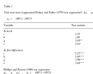
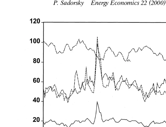
exchange rate is from the Federal Reserve Bank of Saint Louis 1998 data bank. Fig. 1, which plots the actual values of the four series, indicates that none of the series exhibit trends. Consequently, all unit root test regressions were run with a constant but no trend term. Table 1 reports the results from Dickey and Fuller

Ž1979 and Phillips and Perron 1988 unit root tests. The null hypothesis is a unit. Ž . Ž .

root in the series as1 while the alternative hypothesis is a stationary series

Ža/1 . The results from augmented Dickey and Fuller 1979 regressions suggest. Ž .

that at the 1% level of significance, none of the series are stationary in levels. Both

Ž .

the Dickey and Fuller test results and the Phillips and Perron 1988 test results

Table 1

Phillips and Perron 1988 test regression D_{x t}smqax_ty1qut,ts1987:1]1997:9

Critical values from Hamilton 1994 . , , denotes a statistic is significant at the 1%, 5% and 10% level of significance, respectfully. The parameter,l, is a truncated lag parameter used in the non-parametric correction for serial correlation and is set according to the sample size. The

Ž ..

Fig. 1. Energy futures prices and exchange rates.

indicate that each variable is stationary in first differences at the 1% level of significance. Since differencing the data once produces stationarity, I conclude that

Ž Ž ..

each of the series c,h,g, and e is integrated of order 1 I 1 . As discussed in

Ž .

Johansen and Juselius 1990 , while unit root tests are useful guides to the possibility of finding a co-integrating relationship they are not sufficient tests for co-integration. Consequently, it is more useful to test for a common stochastic trend among the time series under consideration. If the variables do share a

Table 2

py1

U U U

a _{Ž .}

Johansen tests for co-integration Dx_ts

Ý

P D_t x_tyt P xtypq«t,yP sab9, xt9s ct,ht,et,gt ts1

Sample period: 1987:1]1997:9, ps6

Eigenvalues 0.2138 0.0996 0.0642 0.0262

Hypothesis rs0 rF1 rF2 rF3

UU

Trace test 56.541 25.510 11.980 3.424

UU

lma xtest 31.031 13.531 8.556 3.424

Co-integrating equation

ztscty1.863htq0.373etq0.796gty0.417

a_{Notes. Ž .} UUU UU U

common stochastic trend then they are co-integrated and an error correction model can be built.

Table 2 reports the values for the lmax and the Trace test statistics. Block exogeneity tests in combination with tests for white noise residuals determined the appropriate lag length as ps6. Both the Trace and l_max test statistics indicate that a co-integration rank of 1 is present. The fact that these three energy futures prices are co-integrated with a trade-weighted exchange rate is important for several reasons. First, this finding of co-integration is important because it means that there exists a long-run equilibrium relationship between these four variables. Second, the existence of co-integration implies that there must be Granger causal-ity between some of the variables. Third, co-integration implies that modelling must be done using a VECM rather than a VAR in first differences.

Ž .

Using Eq. 2 , a VECM model can be represented as

py1

Ž . Ž .

Dxts

_Ý

AtDxtytqazty1q«t, x9ts ct,ht,et,gt 5

ts1

Ž .

where the error correction term ect is given by

Ž .

ztscty1.863 htq0.373 etq0.796 gty0.417 6

Ž .

Eq. 6 can be rearranged so that ct appears on the left-hand side. Since the variables are measured in natural logarithms, the coefficients are elasticities.

Ž .

cts1.863 hty0.373 ety0.796 gtq0.417qzt 6a

Ž .

Eq. 6a indicates that in the long-run equilibrium, a 1% increase in exchange rates lowers crude oil futures prices by 0.373%. This is consistent with Pindyck and

Ž .

Rotemberg 1990 who found that an equally weighted index of the dollar value of British pounds, German marks, and Japanese Yen negatively and significantly

Table 3

Sample period: 1987:1]1997:9, ps6 Dependent variable:

Dc_t Dh_t De_t Dg_t

a 0.119 0.396 y0.021 y0.017

p-value 0.278 6.54ey4 0.498 0.881

Ž .

Q6 0.570 0.610 0.999 0.853

Ž .

Q12 0.239 0.832 0.999 0.240

Ž .

Q24 0.583 0.932 0.952 0.420

a_{Notes. QŽ . Ž . Ž .}

impacts the price of crude oil in both ordinary least squares regressions and latent variable models.

The Johansen procedure can be rather sensitive to residual serial correlation. Consequently, the bottom of Table 3 presents Ljung]Box Q statistics for testing white noise residuals. The reportedQstatistics indicate that the residuals from the VECM are white noise and therefore the VECM specification with ps6 is adequate.

4. Granger causality tests

The upper portion of Table 4 reports probability values for testing short-run

Ž .

Granger causality. These tests can be computed from Eq. 5 by testing the null hypothesis Ai jts0, ts1,2, . . . ,p in the VECM. These hypothesis are tested

Ž .Ž < < < <.

using likelihood ratio tests of the form Tyc log ÝR ylogÝU where T is the number of observations,cis a small sample correction equal to the largest number of parameters estimated in any one of the equations from the VECM and log

<ÝR<and log <ÝU<are the natural logarithms of the determinants of the variance] co-variance matrices from the restricted and unrestricted VECMs, respectively. This statistic is asymptotically distributed as chi-squared with degrees of freedom equal to the number of coefficient restrictions. The null hypothesis of no Granger causality running from the change in the natural logarithm of exchange rates to the change in the natural logarithm of crude oil futures prices can be rejected at the 10% level of significance. The null hypothesis of no Granger causality running from the change in the natural logarithm of exchange rates to the change in the natural logarithm of heating oil futures prices can be rejected at the 5% level of significance. The results in Table 4 also indicate that in the short-run, exchange

Table 4

Granger causality tests

Ž .

Sample period: 1987:1]1997:9 P-values are shown .

Ž .

From: To dependent variable :

Dc_t Dh_t De_t Dg_t

Tests of no short-run Granger causality

Dct 0.019 0.487 0.856 0.040

Dht 0.143 0.324 0.945 0.133

Det 0.099 0.043 0.002 0.316

Dgt 0.182 0.206 0.687 0.346

Tests of no long-run Granger causality

zty1 0.278 6.54ey4 0.498 0.881

Joint tests of no long-run and no short-run Granger causality

rates are primarily driven by their own past values while short-run movements in unleaded gasoline futures prices are primarily driven by movements in crude oil futures prices.

The null hypothesis for testing long-run causal relationships is ais0, is

1, . . . ,4. From Table 4 it is clear that the error correction term is statistically significant at the 1% level in the heating oil equation. These results indicate that the futures prices of heating oil adjust to clear any deviations from long-term disequilibrium.

The fact that the exchange rate equation contains no evidence of either long-run Granger causality or short-run Granger causality suggests that exchange rates are exogenous to the system. The results from formal joint tests of no long-run causality and no short-run causality for each variable are shown in the lower portion of Table 4. The joint hypothesis of no long-run causality and no short-run

Ž .

causality can be rejected at the 5% 1% level of significance for crude oil futures

Ž .

prices heating oil futures prices but cannot be rejected for either exchange rates or unleaded gasoline futures prices. These results suggest that exchange rates transmit exogenous shocks to the system. These results are supportive of the

Ž .

conjecture by Bloomberg and Harris 1995 that recent movements in commodity prices may be a response to movements in the dollar.

5. Stability of the VECM

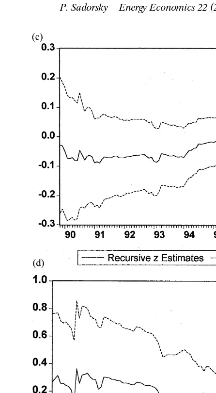
The estimation period for this study covers the somewhat turbulent time of the 1990 Gulf crisis. Consequently, it is important to check the VECM for structural breaks. One way of checking parameter stability is to estimate the VECM recur-sively and plot the recurrecur-sively estimated coefficients, with associated standard error bands, of the error correction terms. Fig. 2A]D show the results from doing this. The plots shown in Fig. 2A]D suggest that a structural stability problem probably does not exist since, for each equation, the size of the estimated coefficients on the error correction terms are fairly similar over the entire sample period.

Ž .

As a further test of parameter stability, I compute Gregory and Hansen 1996 tests for co-integration in models with regime shifts. These tests are designed to test the null hypothesis of no co-integration against the alternative of

co-integra-Ž .

tion in the presence of a possible regime shift. Gregory and Hansen 1996 define four models.

co-integration equation.

w s1 it t)TB _{and 0 otherwise whereT}B _{is the break} tt

date.

Ž .

Model 2: level shift C .

Ž . Ž .

Fig. 2. a Recursive estimates from crude oil equation. b Recursive estimates from heating oil

Ž . Ž .

equation. c Recursive estimates from exchange rate equation. d Recursive estimates from gasoline equation.

Ž .

Model 3: level shift with trend CrT .

y_1tsm₁qm w_{2 tt}qbtqa9₁y_2tqe_t, ts1, . . . ,T

Ž .

y_1tsm₁qm w_{2 tt}qa9₁y_2tqa9₂y_2tw_ttqe_t, ts1, . . . ,T

The computation of the test statistics are straightforward. For each break point,

B _Ž

T , estimate one of the models 2 through 4 depending upon the alternative

. U

hypothesis under consideration by OLS yielding the residuals ett. From these

Ž Ž .

residuals compute the usual augmented Dickey and Fuller test statistic ADFt s

Ž U _.. U _{Ž .}

tstat ety1t and define ADF as the smallest value of the ADFt . The numerical value of ADFU _{can be compared to the critical values tabulated in Gregory and}

Ž .

Hansen 1996 .

Both the ADF and ADFU _{statistics test the null hypothesis of no co-integration.}

Ž . U

Gregory and Hansen 1996 offer some suggestions as to how to use the ADF statistic. Rejection of the null hypothesis of no co-integration by either the

Ž . U

conventional ADF or any other standard test for co-integration or the ADF statistic indicates some long-run equilibrium relationship in the data. If the ADF statistic does not reject but the ADFU _{does reject then structural change may be}

important. If both the ADF and the ADFU _{reject then no information of structural}

change is provided since the ADFU _{is powerful against conventional co-integration.}

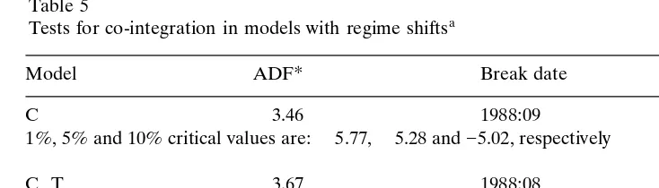
Table 5 reports ADFU _{statistics for testing regime shifts in each of models 2}

through 4. The lag length for the ADFU _{statistics are chosen using Perron’s}

ŽPerron, 1997 t-sig criteria. For illustration purposes consider Eq. 7 .. Ž .

k

U U U _{Ž .}

ettsaety1tq

_Ý

cjDetyjtqut 7

js1

Working backwards from 13 lag lengths, the first value of k is chosen such that thet statistic onck is greater than 1.6 in absolute value and the t statistic oncl for

l)k is less than 1.6 in absolute value. Table 5, which presents the results from testing models 2]4, shows clear evidence against any structural changes in the co-integrating equation. For Model 1, the conventional ADF statistic is ]3.89

Žwhich is significant at the 1% level of significance . Since the ADF, Trace and.

Ž .

l_max test statistics from Table 2 each rejects the null hypothesis of no co-integra-tion, while the ADFU _{statistic doesn’t, it can be concluded that the VECM is a}

structurally stable econometric model.

6. Concluding remarks

The main findings of this study can be summarized as follows. Results are presented showing that futures prices for crude oil, heating oil and unleaded gasoline are co-integrated with a trade-weighted index of exchange rates. This is

Ž .

important because it means that: 1 there exists a long-run equilibrium

relation-Ž .

ship between these four variables; 2 there must be Granger causality between

Ž .

Table 5

a

Tests for co-integration in models with regime shifts U

Model ADF Break date l

C y3.46 1988:09 11

1%, 5% and 10% critical values are:y5.77,y5.28 and]5.02, respectively

CrT y3.67 1988:08 11

1%, 5% and 10% critical values are:y6.05,y5.57 and]5.33, respectively

CrS y3.63 1988:10 11

1%, 5% and 10% critical values are:y6.51,y6.00 and]5.75, respectively

a _{Ž .}

Notes.Critical values from Gregory and Hansen 1996 . The parameter l is set using Perron’s

ŽPerron, 1997 t-sig criterion...

movements in heating oil futures prices in both the long- and short-run while movements in exchange rates precede movements in crude oil futures prices in the short-run. In the long-run equilibrium, a 1% increase in exchange rates lowers crude oil futures prices by 0.373%.

Evidence is also presented that suggests exchange rates transmit exogenous shocks to energy futures prices. This is supportive of the conjecture by Bloomberg

Ž .

and Harris 1995 that recent movements in commodity prices may be a response to movements in the US dollar.

Acknowledgements

This paper was written while I was a Visiting International Scholar at U.C. Davis. I thank Colin Carter for providing me with access to the data and Kathy Edgington for computing assistance. Comments from seminar participants at U.C. Davis, an anonymous referee and Irene Henriques are gratefully acknowledged.

References

Bloomberg, S.B., Harris, E.S., 1995. The commodity]consumer price connection: fact or Fable? Fed. Reserve Board N.Y. Econ. Policy Rev., October, 21]38.

Dickey, D.A., Fuller, W.A., 1979. Distribution of the estimators for autoregressive time series with a

Ž .

unit root. J. Am. Stat. Assoc. 74 366 , 427]431.

Engle, R.F., Granger, C.W.J., 1987. Co-integration and error-correction: representation, estimation, and testing. Econometrica 55, 251]276.

Fama, E., French, K., 1987. Commodity futures prices: some evidence on forecast power, premiums, and the theory of storage. J. Bus. 60, 55]73.

Federal Reserve Board of Saint Louis, 1998. FRED, www.stls.frb.org. Golub, S., 1983. Oil prices and exchange rates. Econ. J. 93, 576]593.

Granger, C.W.J., 1986. Developments in the study of co-integrated economic variables. Ox. Bull. Econ. Stat. 48, 213]228.

Granger, C.W.J., 1988. Some recent developments in the concept of causality. J. Econom. 39, 199]211. Gregory, A.W., Hansen, B.E., 1996. Residual-based tests for cointegration in models with regime shifts.

J. Econ. 70, 99]126.

Hamilton, J.D., 1994. Time Series Analysis. Princeton University Press, Princeton.

Johansen, S., 1988. Statistical analysis of cointegration vectors. J. Econ. Dynam. Control 12, 231]254. Johansen, S., 1991. Estimation and hypothesis testing of cointegrated vectors in Gaussian vector

autoregressive models. Econometrica 59, 1551]1580.

Johansen, S., Juselius, K., 1990. Maximum likelihood estimation and inference on cointegration}with applications to the demand for money. Ox. Bull. Econ. Stat. 52, 169]210.

Ž .

Krugman, P., 1983a. Oil and the dollar. In: Bhandari, J.S., Putnam, B.H. Eds. , Economic Interdepen-dence and Flexible Exchange Rate. Cambridge University Press.

Ž .

Krugman, P., 1983b. Oil shocks and exchange rate dynamics. In: Frankel, J.A. Ed. , Exchange Rates and International Macroeconomics. University of Chicago Press, Chicago.

Perron, P., 1997. Further evidence on breaking trend functions in macroeconomic variables. J. Econom. 80, 355]385.

Phillips, P.C.B., Perron, P., 1988. Testing for a unit root in time series regression. Biometrika 75, 335]346.

Pindyck, R.S., Rotemberg, J.J., 1990. The excess co-movement of commodity prices. Econ. J. 100, 1173]1189.

Prophet Information Services, Inc., 1997. Commodity Data Bank, Mountain View, California.

Ž .

Serlitis, A., 1994. A cointegration analysis of petroleum futures prices. Energy Econ. 16 2 , 93]97. Zhou, S., 1995. The response of real exchange rates to various economic shocks. South. Econ. J. XX,