NASA/TM–2014–218179
FUN3D Manual: 12.4
Robert T. Biedron, Joseph M. Derlaga, Peter A. Gnoffo, Dana P. Hammond,
William T. Jones, Bil Kleb, Elizabeth M. Lee-Rausch, Eric J. Nielsen, Michael A. Park, Christopher L. Rumsey, James L. Thomas, and William A. Wood
Langley Research Center Hampton, Virginia 23681
NASA STI Program . . . in Profile
Since its founding, NASA has been dedicated to the advancement of aeronautics and space science. The NASA scientific and technical information (STI) program plays a key part in helping NASA maintain this important role.
The NASA STI program operates under the auspices of the Agency Chief Information Officer. It collects, organizes, provides for archiving, and disseminates NASA’s STI. The NASA STI
program provides access to the NASA Aeronautics and Space Database and its public interface, the NASA Technical Report Server, thus providing one of the largest collections of aeronautical and space science STI in the world. Results are published in both non-NASA channels and by NASA in the NASA STI Report Series, which includes the following report types:
TECHNICAL PUBLICATION. Reports of completed research or a major significant phase of research that present the results of NASA Programs and include extensive data or theoretical analysis. Includes compilations of significant scientific and technical data and information deemed to be of continuing reference value. NASA counterpart of peer-reviewed formal professional papers, but having less stringent limitations on manuscript length and extent of graphic presentations. TECHNICAL MEMORANDUM. Scientific
and technical findings that are preliminary or of specialized interest, e.g., quick release reports, working papers, and bibliographies that contain minimal annotation. Does not contain extensive analysis.
CONTRACTOR REPORT. Scientific and technical findings by NASA-sponsored contractors and grantees.
CONFERENCE PUBLICATION. Collected papers from scientific and technical conferences, symposia, seminars, or other meetings sponsored or
co-sponsored by NASA.
SPECIAL PUBLICATION. Scientific, technical, or historical information from NASA programs, projects, and missions, often concerned with subjects having substantial public interest.
TECHNICAL TRANSLATION. English-language translations of foreign scientific and technical material pertinent to NASA’s mission.
Specialized services also include organizing and publishing research results, distributing specialized research announcements and feeds, providing information desk and personal search support, and enabling data exchange services. For more information about the NASA STI program, see the following:
Access the NASA STI program home page at http://www.sti.nasa.gov
E-mail your question to [email protected]
Fax your question to the NASA STI Information Desk at 443-757-5803 Phone the NASA STI Information Desk at
443-757-5802 Write to:
STI Information Desk
NASA Center for AeroSpace Information 7115 Standard Drive
NASA/TM–2014–218179
FUN3D Manual: 12.4
Robert T. Biedron, Joseph M. Derlaga, Peter A. Gnoffo, Dana P. Hammond,
William T. Jones, Bil Kleb, Elizabeth M. Lee-Rausch, Eric J. Nielsen, Michael A. Park, Christopher L. Rumsey, James L. Thomas, and William A. Wood
Langley Research Center Hampton, Virginia 23681
National Aeronautics and Space Administration
Langley Research Center Hampton, Virginia 23681
Available from:
NASA Center for AeroSpace Information 7115 Standard Drive
Hanover, MD 21076-1320
The use of trademarks or names of manufacturers in this report is for accurate reporting and does not constitute an official endorsement, either expressed or implied, of such products or manufacturers by the National Aeronautics and Space Administration.
Abstract
This manual describes the installation and execution of FUN3D version 12.4, including optional dependent packages. FUN3D is a suite of computational fluid dynamics simulation and design tools that uses mixed-element unstruc-tured grids in a large number of formats, including strucunstruc-tured multiblock and overset grid systems. A discretely-exact adjoint solver enables efficient gradient-based design and grid adaptation to reduce estimated discretization error. FUN3D is available with and without a reacting, real-gas capability. This generic gas option is available only for those persons that qualify for its beta release status.
Contents
About this Document 9
Acknowledgments 10
Quick Start 11
1 Introduction 15
1.1 Primary Capabilities and Features. . . 15
1.2 Requirements . . . 16 1.3 Grid Generation. . . 16 1.4 Obtaining Fun3D . . . 17 2 Conventions 18 2.1 Compressible Equations . . . 19 2.2 Incompressible Equations. . . 21
2.3 Generic Gas Equations . . . 22
2.4 Unsteady Flows . . . 23
3 Boundary Conditions 24 4 Grids 26 4.1 File Endianness . . . 26
4.2 Supported Grid Formats . . . 26
4.2.1 AFLR3 Grids . . . 27 4.2.2 FAST Grids . . . 27 4.2.3 VGRID Grids . . . 28 4.2.4 FieldView Grids . . . 28 4.2.5 FELISA Grids. . . 29 4.2.6 Fun2DGrids . . . 29
4.3 Translation of Additional Grid Formats . . . 30
4.3.1 PLOT3D Grids . . . 30
4.3.2 CGNS Grids . . . 31
5 Flow Solver, nodet 33 5.1 Flow Solver Execution . . . 33
5.2 Command Line Options . . . 33
5.3 Output Files . . . 34
5.3.1 Flow Visualization . . . 34
6 Adjoint Solver, dual 36
6.1 Convergence of the Linear Adjoint Equations. . . 36
6.2 Required Directory Hierarchy and Executing dual . . . 36
6.3 rubber.data . . . 37
6.4 Output Files . . . 38
7 Grid Adaptation 39 7.1 Geometry Specification and Grid Freezing for refine . . . 39
7.1.1 No geometry, where the surface nodes are frozen. . . . 39
7.1.2 FAUXGeom for Planar Boundaries . . . 40
7.2 Performing Feature-Based Adaptation . . . 40
7.3 Performing Adjoint-Based Adaptation . . . 40
7.4 Scripting Grid Adaptation . . . 41
7.4.1 Input File case specifics forf3d Script . . . 41
8 Design Optimization 44 8.1 Objective/Constraint Functions . . . 45
8.1.1 Terminology . . . 45
8.1.2 Functional Form . . . 46
8.2 Some Details on Specific Objective/Constraint Functions . . . 48
8.2.1 Lift-to-Drag Ratio (Keyword: clcd) . . . 48
8.2.2 Rotorcraft Figure of Merit (Keyword: fom) . . . 48
8.2.3 Rotorcraft Propulsive Efficiency (Keyword: propeff) . 49 8.2.4 RMS of Stagnation Pressure (Keyword: pstag) . . . . 49
8.2.5 Near-field Targetp/p∞ (Keyword: boom targ) . . . 49
8.2.6 CoupledsBOOMGround-Based Signatures, Noise Met-rics, and Equivalent Areas (Keyword: sboom) . . . 51
8.2.7 Supersonic Mach Cut Equivalent Area Distribution (Key-word: ae) . . . 52
8.2.8 Target Pressure Distributions (Keyword: cpstar) . . . 53
8.3 Geometry Parameterizations . . . 53
8.3.1 Surface Grid Extraction . . . 54
8.3.2 Access to Executables . . . 54
8.3.3 Notes on Using Sculptor . . . 55
8.3.4 Using Other Parameterization Packages. . . 55
8.4 Design Optimization Directory Structure . . . 56
8.5 Contents of theammo Directory . . . 56
8.5.1 ammo.input . . . 57
8.6 Contents of thedescription.i Directory . . . 59
8.6.1 Geometry Parameterization Files . . . 60
8.6.2 rubber.data . . . 62
8.6.4 body grouping.data(optional) . . . 68
8.6.5 command line.options (optional). . . 69
8.6.6 cpstar.data.j (optional) . . . 70
8.6.7 machinefile(optional) . . . 70
8.6.8 pressure target.dat (optional) . . . 70
8.6.9 transforms.i (optional) . . . 70
8.7 Contents of themodel.i Directory . . . 70
8.8 Running the Optimization . . . 71
8.8.1 Filesystem Latency Problems . . . 72
8.9 Multi-objective Design . . . 72
8.9.1 KSOPT . . . 73
8.9.2 PORT, SNOPT . . . 73
8.10 Multi-point Design . . . 73
8.10.1 Linear Combination of Objective Functions. . . 74
8.10.2 Combination of Objective Functions using the Kreisselmeier-Steinhauser Function . . . 75
8.10.3 Single-Point Objective Function with Off-Design Con-straint Functions . . . 75
8.11 Optimization of Two-Dimensional Geometries . . . 75
8.12 Using a Different Optimization Package . . . 76
8.13 Implementing New Cost Functions/Constraints . . . 77
8.14 Forward Mode Differentiation Using Complex Variables . . . 77
References 79 A Installation 85 A.1 Extracting Files . . . 85
A.2 Configure Introduction . . . 85
A.3 Alternative Installation Path . . . 86
A.4 Fortran Compiler Option Tuning (FTune) . . . 86
A.5 Complex Variable Version . . . 87
A.6 Internal Libraries . . . 87
A.6.1 KNIFE. . . 87
A.6.2 REFINE . . . 87
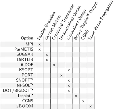
A.7 External Libraries . . . 87
A.7.1 MPI . . . 88
A.7.2 ParMETIS. . . 89
A.7.3 SUGGAR++-1.0.10 or Higher . . . 90
A.7.4 DiRTlib v1.40 or higher . . . 90
A.7.5 6-DOF . . . 91
A.7.6 KSOPT . . . 91
A.7.8 SNOPT . . . 91 A.7.9 NPSOL . . . 92 A.7.10 DOT/BIGDOT . . . 92 A.7.11 Tecplot . . . 92 A.7.12 CGNS . . . 93 A.7.13 sBOOM. . . 93
B Fun3D Input Files 94 B.1 stop.dat . . . 94
B.2 [project rootname].flow . . . 95
B.3 remove boundaries from force totals . . . 95
B.4 fun3d.nml . . . 95
B.4.1 &project . . . 97
B.4.2 &raw grid . . . 98
B.4.3 &force moment integ properties . . . 100
B.4.4 &governing equations . . . 101
B.4.5 &reference physical properties . . . 104
B.4.6 &inviscid flux method . . . 106
B.4.7 &turbulent diffusion models . . . 110
B.4.8 &spalart . . . 112
B.4.9 &code run control . . . 113
B.4.10 &nonlinear solver parameters . . . 116
B.4.11 &linear solver parameters . . . 119
B.4.12 &boundary conditions . . . 120 B.4.13 &component parameters . . . 133 B.4.14 &two d trans . . . 135 B.4.15 &three d trans . . . 137 B.4.16 &special parameters . . . 138 B.4.17 &flow initialization . . . 139
B.4.18 &time avg params . . . 141
B.4.19 &global . . . 142
B.4.20 &volume output variables . . . 144
B.4.21 &boundary output variables . . . 154
B.4.22 &sampling output variables . . . 166
B.4.23 &sampling parameters . . . 177
B.4.24 &slice data . . . 186
B.4.25 &massoud output . . . 196
B.4.26 &overset data . . . 199
B.4.27 &rotor data . . . 201
B.4.28 &adapt metric construction . . . 202
B.4.29 &adapt mechanics . . . 207
B.4.30 &sonic boom . . . 212
B.4.32 &equivalent area . . . 222
B.4.33 &noninertial reference frame . . . 223
B.5 moving body.input . . . 225
B.5.1 &body definitions . . . 226
B.5.2 &forced motion . . . 230
B.5.3 &observer motion . . . 234
B.5.4 &motion from file . . . 237
B.5.5 &surface motion from file . . . 239
B.5.6 &sixdof motion . . . 240
B.5.7 &aeroelastic modal data . . . 243
B.5.8 &composite overset mesh. . . 246
B.5.9 &grid transform . . . 247
B.6 rotor.input . . . 249
B.6.1 Header . . . 251
B.6.2 Actuator Surface Model . . . 251
B.6.3 Rotor Reference System . . . 252
B.6.4 Rotor Loading. . . 253
B.6.5 Blade Parameters . . . 254
B.6.6 Blade Element Parameters for Load Type=3 . . . 254
B.6.7 Pitch Control Parameters for Load Type=3 . . . 255
B.6.8 Prescribed Flap Parameters . . . 256
B.6.9 Prescribed Lag Parameters . . . 256
B.7 tdata . . . 257
B.7.1 perfect gas Keyword . . . 257
B.7.2 equilibrium air tKeyword . . . 257
B.7.3 equilibrium air rKeyword . . . 258
B.7.4 oneKeyword . . . 258
B.7.5 twoKeyword . . . 258
B.7.6 FEMKeyword . . . 259
B.8 species thermo data . . . 259
B.9 kinetic data . . . 262
B.10 species transp data . . . 263
B.11 species transp data 0 . . . 264
B.12 hara namelist data . . . 265
C Troubleshooting 272 C.1 What if the solver has trouble starting or reports NaNs? . . . 272
C.2 What if the forces and moments aren’t steady or residuals don’t converge to steady-state? . . . 272
C.3 What if the solver dies unexpectedly? . . . 273 C.4 What if a segmentation fault occurs after “Calling ParMetis”? 273
C.5 What if the solver dies with an error like “input statement re-quires too much data” after echoing the wrong number of ele-ments or nodes? . . . 273 C.6 What if the solver dies with an error like “input statement
re-quires too much data” after echoing the number of tetrahedra and nodes for a VGRIDmesh? . . . 273 C.7 What if the solver reports that the Euler numbers differ? . . . 273 C.7.1 Euler Number Description . . . 274 C.7.2 Determining the Impact of an Euler Number Mismatch 275
About this Document
This manual is intended to guide an application engineer through configura-tion, compiling, installing, and executing theFun3Dsimulation package. The
focus is on the most commonly exercised capabilities. Therefore, some of the immature or rarely exercised capabilities are intentionally omitted in the in-terest of clarity. An accompanying document that provides example cases is under development.
Release of the generic gas capability is restricted because of International Traffic in Arms Regulations (ITAR), so Fun3D usually distributed with the
generic gas capability disabled. See section 1.4 for details. This manual de-scribesFun3Dwith and without the generic gas capability, denotedeqn type= ’generic’. Features that are specific to aneqn type are explicitly indicated. This document is updated and released with each subsequent version of
Fun3D. In fact, a significant portion is automatically extracted from the Fun3D source code. If you have difficulties, find any errors, or have any
suggestions for improvement please contact the authors at
Acknowledgments
A large portion of this content originated as a web-based manual, which con-tained contributions from Eric Nielsen, Elizabeth Lee-Rausch, Jan-Renee Carl-son, Karen Bibb, Bill Jones, Jeff White, Eric Lynch, Dave O’Brien, Mari-lyn Smith, and Clara Helm. Sriram Rallabhandi provided the description of
sBOOM. The namelist documentation is parsed from Fun3D source code,
which is written by the developers. Contributors to Fun3Dinclude
Ponnam-palam (Bala) Balakumar, Karen Bibb, Bob Biedron, Jan Carlson, Mark Car-penter, Peter Gnoffo, Dana Hammond, Bill Jones, Bil Kleb, Beth Lee-Rausch, Eric Nielsen, Hiroaki Nishikawa, Mike Park, Chris Rumsey, Jim Thomas, Veer Vatsa, Jeff White, Alejandro Campos, Rajiv Shenoy, Marilyn Smith, Joe Derlaga, Natalia Alexandrov, W. Kyle Anderson, Harold Atkins, Bill Wood, Austen Duffy, Clara Helm, Chris Cordell, Kyle Thompson, Hicham Alkandry, Shelly Jiang, Eric Lynch, Jennifer Abras, Nicholas Burgess, Dave O’Brien, Tommy Lambert, Ved Vyas, Shatra Reehal, Kan Yang, Andrew Sweeney, Brad Neff, Genny Pang, Gregory Bluvshteyn, Dan Gerstenhaber, Geoff Parsons, and Rena Rudavsky.
Quick Start
This section takes you from source code tarball to a rudimentary flow so-lution using single processor execution on a typical Unix-style environment (e.g. Linux, Mac® OS) with a Fortran compiler and the GNU Make utility.
Fun3D is most commonly executed in parallel, but the intent here is to
pro-vide the most basic installation, setup, and execution of theFun3Dflow solver
without the complexity of any third-party libraries or packages.
See section1.4for instructions on obtaining theFun3Dsource code tarball. Once you have it, unpack the source code tarball, configure it for your system (sectionA), compile it, and add the executables directory to your search path. For C Shell, e.g.,
tar zxf fun3d-12.4.tar.gz cd fun3d-12.4 mkdir _seq cd _seq ../configure --prefix=${PWD} make install
setenv PATH ${PWD}/bin:${PATH} cd ..
For Bourne Shell, thesetenvcommand isexport PATH=${PWD}/bin:${PATH}. The change to the PATH environment variable can be made permanently by adding thesetenv orexport command to your shell start up file. Next, move to the doc/quick startdirectory,
cd doc/quick_start
where you will find a very coarse 3D wing grid (inv wing.fgrid) intended for inviscid flow simulation (section 4). Also in this directory are the associated boundary conditions file inv wing.mapbc (section 3) and a Fun3D input file
fun3d.nml in Fortran namelist format (section B.4).
Execute the flow solver (section 5.1) by running the command
nodet
This should produce screen output similar to
1 FUN3D 12.4-70107 Flow started 03/31/2014 at 10:33:12 with 1 processes
2 Contents of fun3d.nml file
below---3 &project 4 project_rootname = 'inv_wing' 5 / 6 &raw_grid 7 grid_format = 'fast' 8 data_format = 'ascii' 9 / 10 &governing_equations 11 viscous_terms = 'inviscid'
12 / 13 &reference_physical_properties 14 mach_number = 0.7 15 angle_of_attack = 2.0 16 / 17 &code_run_control 18 restart_read = 'off' 19 steps = 150 20 stopping_tolerance = 1.0e-12 21 / 22 &global 23 boundary_animation_freq = -1 24 /
25 Contents of fun3d.nml file
above---26 rotor.input not found
27
28 moving_body.input not found
29 moving_body.input not found
30 ... opening inv_wing.fgrid
31 ... nnodesg: 6309 ntet: 35880 ntface: 1392
32
33 cell statistics: type, min volume, max volume, max face angle
34 cell statistics: tet, 0.38305628E-05, 0.14174467E+02, 143.526944837
35 cell statistics: all, 0.38305628E-05, 0.14174467E+02, 143.526944837
36
37 ... Constructing partition node sets for level-0... 35880 T
38 ... Edge Partitioning ....
39 ... Boundary partitioning....
40 ... Reordering for cache efficiency....
41 ... Write global grid information to inv_wing.grid_info
42 ... Time after preprocess TIME/Mem(MB): 0.71 100.15 100.15
.. .
197 Lift 0.809996568758631E-01 Drag 0.107734796873048E-01
198 77 0.347515632356081E-12 0.16460E-10 0.26803E+01 0.00000E+00 -0.62327E+00
199 Lift 0.809996568770187E-01 Drag 0.107734796873170E-01
200 78 0.264078581490539E-12 0.12961E-10 0.26803E+01 0.00000E+00 -0.62327E+00
201 Lift 0.809996568779106E-01 Drag 0.107734796873263E-01
202 79 0.201939553281957E-12 0.10194E-10 0.26803E+01 0.00000E+00 -0.62327E+00
203 Lift 0.809996568785974E-01 Drag 0.107734796873335E-01
204
205 Writing boundary output: inv_wing_tec_boundary.dat
206 Time step: 79, ntt: 79, Prior iterations: 0
207
208 Writing inv_wing.flow (version 11.8) lmpi_io 2
209 inserting current history iterations 79
210 Time for write: 0.0 s
211 Done.
If Fun3D completed successfully, a Mach 0.7 inviscid flow over a very
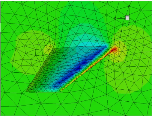
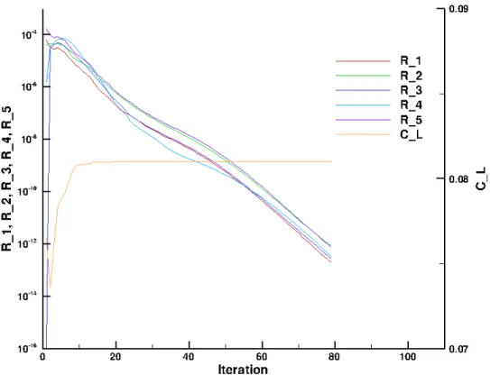
coarse representation of an ONERA M6 semi-span wing [1] at two degrees angle of attack is available. If not, please refer to Troubleshooting on page272. With visualization software capable of reading Tecplotfiles, you can visu-alize various surface quantities with inv wing tec boundary.datas shown by the pressure contours in Fig. 1. Iterative convergence history can be plotted from inv wing hist.dat as shown in Fig. 2. Histories of all five conservation equation residual norms are denoted R 1–R 5, and the lift coefficient conver-gence history is denoted C L.
Figure 1: Mach 0.7 flow about a coarse ONERA M6 semi-span wing at 2 degrees angle of attack.
1
Introduction
Fun3D began as a research code in the late 1980s. [2] The code was created
to develop new algorithms for unstructured-grid fluid dynamic simulations of incompressible and compressible transonic flows. The project has since grown into a suite of codes that cover not only flow analysis, but adjoint-based error estimation, mesh adaptation, and design optimization of fluid dynamic problems extending into the hypersonic regime. [3]
Fun3D is currently used as a production flow analysis and design tool to
support NASA programs. Continued research efforts have also benefited by the improvements to stability, ease of use, portability, and performance that this shift to simultaneous support of development and production environments has required. These benefits also include the rapid evaluation of new techniques on realistic simulations and a rapid maturation of experimental techniques to production-level capabilities.
1.1
Primary Capabilities and Features
The primary capabilities of Fun3Dare:
Parallel domain decomposition with Message Passing Interface (MPI) communication for distributed computing
Two-dimensional (2D) and Three-dimensional (3D) node-based, finite-volume discretization
Thermodynamic models: perfect gas (compressible and incompressible) and thermochemical equilibrium, and non-equilibrium1
Time-accurate options from first- to fourth-order with temporal error controllers
Upwind flux functions: flux difference splitting, flux vector splitting, artificially upstream flux vector splitting, Harten-Lax-van Leer contact, low dissipation flux splitting scheme, and others
Turbulence models: Spalart-Allmaras, Menter omega SST, Wilcox k-omega, detached eddy simulation, and others, including specified or pre-dicted transition
Multigrid with implicit time stepping where the linear system is solved using either point-implicit, line-implicit, or Newton-Krylov
Propulsion simulation including inlets, nozzles, and system performance
1The multi-species, thermochemical non-equilibrium capability requires the high-energy
physics library, which is only made available upon specific request and under certain condi-tions, see section1.4for details.
Grid motion: time-varying translation, rotation, and deformation includ-ing overset meshes and six degrees of freedom trajectory computations
Adjoint- and feature-based grid adaptation
Gradient based sensitivity analysis and design optimization via hand-coded discrete adjoint for reverse mode differentiation and automated complex variables for forward mode differentiation
Before exploring more advanced applications (e.g., grid adaptation, moving grids, overset grids, design optimization), the user should become familiar with
Fun3D’s basic flow solving capabilities and have appropriate computational
capability available as indicated in the next section.
1.2
Requirements
TheFun3Ddevelopment team’s typical computing platform is Linux clusters;
so this is the most thoroughly tested environment for the software. A number of users also run on other UNIX-like environments including Mac OS X; these platforms are supported as well. Users have also run on other architectures such as Microsoft Windows-based PC’s; however, the team cannot provide explicit support for these environments.
The user will need GNU Make and a Fortran compiler that supports at least the Fortran 95 standard. During configuration, the Fortran compiler is tested, and any newer Fortran features or extensions are detected are used to the greatest extent possible. A large number of compilers are tested by an automated build framework, including Intel®, Portland Group®, NAG®, Lahey/Fujitsu®, Cray®, Absoft®, IBM®, GFortran, and G95.
While the code can be compiled to run on only a single processor, as demon-strated in the Quick Start section, most applications will require compiling against an MPI implementation and the ParMETIS domain decomposition library to allow parallel execution.
The flow solver uses approximately 2.4 kilobytes of memory per grid point for a perfect gas RANS simulation with a loosely-coupled turbulence model. For example, a grid with one million mesh points would require approximately 2.4 gigabytes of memory. Memory usage will increase slightly with the in-crease in the number of processors because of the increasing boundary data exchanged. Different solution algorithms and co-visualization options will also require additional memory. Typically, one CPU core per 50,000 grid points is suggested, where a 3D mesh of 20 million grid points would require 400 cores.
1.3
Grid Generation
Fun3Dhas no grid generation capability. For internal development at NASA,
Langley), SolidMesh/AFLR3 (Mississippi State), Pointwise (Pointwise, Inc.), and GridEx (NASA Langley).
For 2D grids, the development team normally uses the AFLR2 software written by Dave Marcum et al. at Mississippi State University. Scripts are available to facilitate the use of this grid generator, but the generator itself must be obtained from Marcum. BAMG is also used for 2D grid generation and adaptation.
1.4
Obtaining
Fun3D
Fun3D is export restricted and can only be given to a “U.S. Person,” which
is a citizen of the United States, a lawful permanent resident alien of the U.S., or someone in the U.S. as a protected political asylee or under amnesty. The word “person” includes U.S. organizations and entities, such as companies or universities, see 22 CFR §120.15 for the full legal definition. Release of the high-energy, real-gas capability is further restricted because of International Traffic in Arms Regulations (ITAR).
To request the Fun3D software suite, which will include the refine grid
adaptation and mesh untangling library and the knife cut-cell library, please
use the website request form available at
http://fun3d.larc.nasa.gov/chapter-1.html#request fun3d
or send an email [email protected] the following infor-mation:
“U.S. person” to put on agreement form, i.e., an institution or individual
Point of contact (if “U.S. Person” is not an individual)
Point of contact email address
Phone number, extension
FAX number (if available)
Address (PO boxes not allowed)
Proposed application2 (optional)
How did you discover Fun3D? (optional)
After some background checks to verify that you qualify as a “U.S. Person,” you will be sent a software usage agreement form. Once a completed us-age agreement form is received and the Fun3D support team is notified, the Fun3Dsupport team will make arrangements for transfer of theFun3D
soft-ware suite.
2The high-energy physics library that allows multiple species and non-equilibrium
chem-istry are only included upon specific request—be sure to note that you desire access to this beta functionality as part of your application.
2
Conventions
This chapter discusses the coordinate system orientation and nondimension-alization used by Fun3D. The nomenclature for this section is
a = Speed of sound C = Sutherland constant
e = Energy per unit mass f = Frequency
h = Enthalpy per unit mass k = Thermal conductivity L = Length M = Mach number p = Pressure R = Gas constant Re = Reynolds number t = Time T = Temperature
u, v, w = Cartesian components of velocity x, y, z = Cartesian directions
α = Angle of attack β = Angle of sideslip γ = Heat capacity ratio µ = Viscosity
ρ = Density
where an asterisk (∗) denotes a dimensional quantity. A subscript ref de-notes a reference quantity. For fluid variables, such as pressure, ref usually corresponds to the value ‘at ∞’ for external flows or another condition for internal flows. The units of various reference quantities must be consistent. For example, if the reference speed of sound is defined in feet/sec, then the dimensional reference length, L∗ref, must be in feet. In what follows, L∗ref is
the length in the grid that corresponds to the dimensional reference length; Lref is considered dimensionless.
Fun3D’s angle of attack, sideslip angle, and associated force coefficients
are based on a body-fixed coordinate system:
positive x is toward the back of the vehicle;
positive z is upward
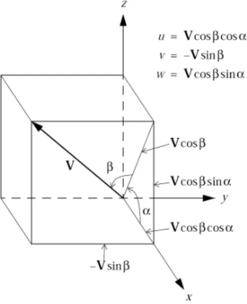
as shown in Fig. 3. This differs from the standard wind coordinate system by a 180 degree rotation about the y axis. The α and β flow angle conventions are shown in Fig. 4.
Figure 3: Fun3Dbody coordinate system.
Figure 4: Fun3D freestream flow angle definition.
2.1
Compressible Equations
x = x∗/(L∗ref/Lref)
y = y∗/(L∗ref/Lref)
z = z∗/(L∗ref/Lref)
t = t∗a∗ref/(L∗ref/Lref)
|V| = |V∗|/a∗ref |V|ref = Mref
u = u∗/a∗ref uref = Mrefcosαcosβ
v = v∗/a∗ref vref = −Mrefsinβ
w = w∗/a∗ref wref = Mrefsinαcosβ
p = p∗/(ρ∗refa∗2ref) pref = 1/γ
a = a∗/a∗ref aref = 1
T = T∗/T∗ref Tref = 1
e = e∗/(ρ∗refa∗ref2 ) eref = 1/(γ(γ−1)) +Mref2 /2
To see how the nondimensional Navier-Stokes equations that are solved in Fun3D are obtained from their dimensional counterparts, it is sufficient to look at the unsteady, one-dimensional equations for conservation of mass, momentum, and energy:
∂ρ∗ ∂t∗ + ∂(ρ∗u∗) ∂x∗ = 0 ∂(ρ∗u∗) ∂t∗ + ∂ ∂x∗ ρ∗u∗2+p∗− 4 3µ ∗∂u∗ ∂x∗ = 0 ∂e∗ ∂t∗ + ∂ ∂x∗ (e∗+p∗)u∗−4 3µ ∗ u∗∂u ∗ ∂x∗ −k ∗∂T∗ ∂x∗ = 0
where k∗ is the thermal conductivity. For a thermally and calorically perfect gas, we also have the equation of state, the definition of the speed of sound, and the specific heat relation:
T∗ = p ∗
ρ∗R∗
a∗2 =γR∗T∗ (γ =cp∗/cv∗)
cp∗+cv∗ =R∗ R∗/cp∗ = (γ−1)/γ
The laminar viscosity is related to the temperature via Sutherland’s law
µ∗ =µ∗refT ∗ ref +C∗ T∗ +C∗ T∗ T∗ ref 3/2
where C∗ = 198.6◦R for air.
Substitution of the nondimensional variables defined above into the equa-tion of state and the definiequa-tion of the speed of sound gives:
T = γp ρ =a
Sutherland’s law in nondimensional terms is given by µ= 1 +C
T +CT
3/2
where C = 198.6◦R/T∗ref and where T∗ref is in degrees Rankine.
Substitution of the dimensionless variables into the conservation equations gives, after some rearrangement,
∂ρ ∂t + ∂(ρu) ∂x = 0 ∂(ρu) ∂t + ∂ ∂x ρu2 +p− 4 3 Mref ReLref µ∂u ∂x = 0 ∂e ∂t + ∂ ∂x (e+p)u− 4 3 Mref ReLref µu∂u ∂x − Mref ReLrefPr(γ−1) µ∂T ∂x = 0 where Pr is the Prandtl number (generally assumed to be 0.72 for air)
Pr =
c∗p µ∗ k∗
and where ReLref, the Reynolds number per unit length in the grid, corre-sponds to the input variablereynolds numberin thefun3d.nmlfile. ReLref is related to the Reynolds number characterizing the physical problem, ReL∗
ref by
ReLref =
ρ∗ref|V∗|ref(L∗ref/Lref)
µ∗ ref = ρ ∗ ref|V∗|refL ∗ ref µ∗ ref 1 Lref = ReL∗ref Lref
2.2
Incompressible Equations
x = x∗/(L∗ref/Lref) y = y∗/(L∗ref/Lref) z = z∗/(L∗ref/Lref)t = t∗|V∗|ref/(L∗ref/Lref)
|V| = |V∗|/|V∗|ref |V|ref = 1
u = u∗/|V∗|ref uref = cosαcosβ
v = v∗/|V∗|ref vref = −sinβ
w = w∗/|V∗|ref wref = sinαcosβ
For incompressible flows, Fun3D does not model any heat sources. The
temperature T∗ is constant and so is the viscosityµ∗. After dividing through by a constant reference density, the one-dimensional continuity and momentum equations are: ∂u∗ ∂x∗ = 0 ∂u∗ ∂t∗ + ∂ ∂x∗ u∗2+ p ∗ ρ∗ ref −4 3 µ∗ref ρ∗ ref ∂u∗ ∂x∗ = 0
The fundamental difference between the nondimensionalization of the com-pressible equations and the incomcom-pressible equations is that the sound speed is used in the former and the flow speed in the latter. Substitution of the dimensionless variables defined above into the conservation equations gives, after some rearrangement,
∂u ∂x = 0 ∂u ∂t + ∂ ∂x u2+p− 4 3 1 ReLref ∂u ∂x = 0
where, exactly the same as in the compressible-flow path, the Reynolds number per unit length in the grid is
ReLref =
ρ∗ref|V∗|refL∗ref
µ∗
ref
= ReL∗ref Lref
2.3
Generic Gas Equations
The generic gas path requires all reference quantities (velocity, density, temper-ature) be entered in the meter-kilogram-second (MKS) system. The transport property nondimensionalization includes the effects of rescaling using the grid length conversion factor. The nondimensionalization of other flow variables follows the practice used to derive the Mach number independence principle. Neither Mach number nor Reynolds number can be used to define reference conditions; these are derived from the fundamental reference quantities. The derived Reynolds number is relative to a one meter reference length. Tem-perature is never non-dimensionalized; it always appears in units of degrees Kelvin.
ρ = ρ∗/ρ∗ref ρ∗ref [kg/m3]
u = u∗/V∗ref Vref∗ [m/s]
v = v∗/V∗ref Tref∗ [K]
a = a∗/V∗ref
p = p∗/(ρ∗refV∗2ref) e = e∗/V∗2ref
h = h∗/V∗2ref
µ = µ∗(T∗)/ρ∗refVref∗ L∗ref
2.4
Unsteady Flows
One of the challenges in unsteady flow simulation is determining the nondi-mensional time step ∆t. The number of time steps at that ∆t necessary to resolve the lowest frequency of interest will impact the cost of the simulation and too large a ∆t will corrupt the results with temporal errors. Time is non-dimensionalized within Fun3Dby
t = t∗a∗ref/(L∗ref/Lref) (compressible)
t = t∗|V∗|ref/(L∗ref/Lref) (incompressible)
where, as in the previous sections, quantities denoted with ∗ are dimensional. In all unsteady flows, one or more characteristic times t∗chr may be
identi-fied. In a flow with a known natural frequency of oscillation (e.g., vortex shed-ding from a cylinder), or in situations where a forced oscillation is imposed (e.g., a pitching wing), a dominant characteristic time is readily apparent. In such cases, if the characteristic frequency in Hz (cycles/sec) is f∗chr, then
t∗chr = 1/f∗chr
In other situations, no oscillatory frequency may be apparent (or not known a priori). In such cases, the time scale associated with the time it takes for a fluid particle (traveling at a nominal speed of |V∗|ref) to pass the body of reference length L∗ref is often used:
t∗chr = L∗ref/|V∗|ref
The corresponding nondimensional characteristic time is therefore given by: tchr = t∗chra∗ref/(L∗ref/Lref) (compressible)
tchr = t∗chr|V∗|ref/(L∗ref/Lref) (incompressible)
Once the nondimensional characteristic tchr is determined, the user must
decide on an appropriate number of time steps (N) to be used for resolving that characteristic time. Then the nondimensional time step may be specified as:
∆t = tchr /N
The proper value ofN must be determined by the user. However, a reasonable rule of thumb for second-order time integration is to takeN = 200. Note that if there are multiple frequencies requiring resolution in time, the most restrictive should be used to determine ∆t.
3
Boundary Conditions
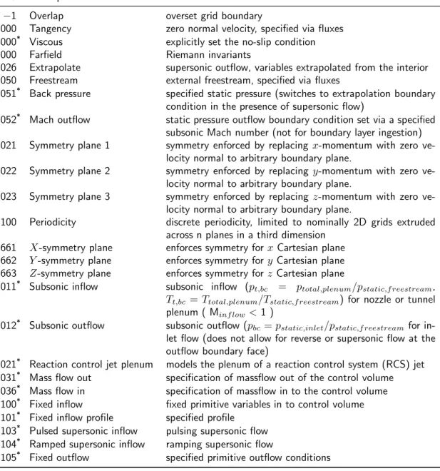
This chapter discusses the boundary conditions available in Fun3D. Table 1 lists the integers used to specify Fun3D boundary conditions with a short
description. Each grid description subsection in section4 indicates how these integers are specified. Details of the boundary condition implementation are provided by Carlson. [4] Some boundary conditions have required or option-ally specified parameters defined in the &boundary conditions namelist, see section B.4.12for further boundary condition details.
Table 1: Fun3Dboundary conditions.
BC Description Notes
−1 Overlap overset grid boundary
3000 Tangency zero normal velocity, specified via fluxes 4000* Viscous explicitly set the no-slip condition
5000 Farfield Riemann invariants
5026 Extrapolate supersonic outflow, variables extrapolated from the interior 5050 Freestream external freestream, specified via fluxes
5051* Back pressure specified static pressure (switches to extrapolation boundary
condition in the presence of supersonic flow)
5052* Mach outflow static pressure outflow boundary condition set via a specified
subsonic Mach number (not for boundary layer ingestion) 6021 Symmetry plane 1 symmetry enforced by replacingx-momentum with zero
ve-locity normal to arbitrary boundary plane.
6022 Symmetry plane 2 symmetry enforced by replacingy-momentum with zero ve-locity normal to arbitrary boundary plane.
6023 Symmetry plane 3 symmetry enforced by replacing z-momentum with zero ve-locity normal to arbitrary boundary plane.
6100 Periodicity discrete periodicity, limited to nominally 2D grids extruded across n planes in a third dimension
6661 X-symmetry plane enforces symmetry forxCartesian plane 6662 Y-symmetry plane enforces symmetry fory Cartesian plane 6663 Z-symmetry plane enforces symmetry forzCartesian plane 7011* Subsonic inflow subsonic inflow (p
t,bc = ptotal,plenum/pstatic,f reestream,
Tt,bc =Ttotal,plenum/Tstatic,f reestream) for nozzle or tunnel
plenum ( Minf low<1 )
7012* Subsonic outflow subsonic outflow (pbc=pstatic,inlet/pstatic,f reestream for
in-let flow (does not allow for reverse or supersonic flow at the outflow boundary face)
7021* Reaction control jet plenum models the plenum of a reaction control system (RCS) jet
7031* Mass flow out specification of massflow out of the control volume
7036* Mass flow in specification of massflow in to the control volume 7100* Fixed inflow fixed primitive variables in to control volume
7101* Fixed inflow profile specified profile
7103* Pulsed supersonic inflow pulsing supersonic flow 7104* Ramped supersonic inflow ramping supersonic flow
7105* Fixed outflow specified primitive outflow conditions *See
&boundary conditions namelist in section B.4.12 to specify auxiliary information and for further descriptions.
4
Grids
This chapter explains how to supply the proper file formats to Fun3D, but does not cover how to create a mesh. See section 1.3 for grid generation guidance. Fun3Dsupports a direct reader for many grid formats. The format
of the grid is specified in the &raw grid namelist. In addition to the directly read formats, translators are provided to convert additional grid formats into a format that can be read directly, see section 4.3.
4.1
File Endianness
The ordering of bytes within a data item is known as “endianness.” If the endianness of a file is different than the native endianness of the computer then a conversion must be performed. The endianness of each grid file format is described in section 4.2. If your compiler supports it, Fun3Dwill attempt
to open binary files with aopen(convert=...)keyword extension. Consult the documentation of the Fortran compiler you are using to determine if other methods are available. For example, with the Intel®Fortran compiler, the en-dianness of file input and output can be controlled by setting theF UFMTENDIAN
environment variable to big orlittle.
4.2
Supported Grid Formats
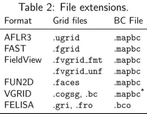
Fun3Dnatively supports the grid formats summarized in Table 2.
Table 2: File extensions.
Format Grid files BC File
AFLR3 .ugrid .mapbc
FAST .fgrid .mapbc
FieldView .fvgrid fmt .mapbc .fvgrid unf .mapbc
FUN2D .faces .mapbc
VGRID .cogsg,.bc .mapbc*
FELISA .gri,.fro .bco
*Same suffix, but GridTool format.
The standard Fun3D .mapbc file format contains the boundary condition information for the grid. The first line is an integer corresponding to the num-ber of boundary groups contained in the grid file. Each subsequent line in this file contains two integers, the boundary face number and the Fun3D
bound-ary condition integer; these numbers may optionally be followed by a character string that specifies a “family” name for the boundary. The family name is required if the patch lumping option (section B.4.2) is invoked to combine
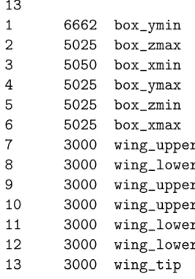
patches into fewer patch families. Below is a sample .mapbcfile illustrative for all grid formats except GridTool/VGRID, FELISA, and FUN2D, which are
described later. 13 1 6662 box_ymin 2 5025 box_zmax 3 5050 box_xmin 4 5025 box_ymax 5 5025 box_zmin 6 5025 box_xmax 7 3000 wing_upper 8 3000 wing_lower 9 3000 wing_upper 10 3000 wing_upper 11 3000 wing_lower 12 3000 wing_lower 13 3000 wing_tip 4.2.1 AFLR3 Grids
AFLR3, SolidMesh, Pointwise, and GridEx can all produce this format and
Fun3Dships with translators that convert Plot3D and CGNS grids to AFLR3
format. The format is documented online athttp://simcenter.msstate.edu/ docs/solidmesh/ugridformat.html
AFLR3 grid file format types are indicated by file suffixes. The formatted (plain text) style has a .ugridsuffix while other types vary according to endi-anness (see section 4.1) and binary type as shown in Table 3. The boundary
Table 3: AFLR3 non-ASCII grid suffixes.
Type Little endian Big endian
Fortran Stream, C Binary .lb8.ugrid .b8.ugrid
Fortran Unformatted .lr8.ugrid .r8.ugrid
conditions are specified via the standardFun3D .mapbc format.
4.2.2 FAST Grids
The .fgrid file contains the complete grid stored in ASCII FAST format. The format is documented online at http://simcenter.msstate.edu/docs/ solidmesh/FASTformat.html The boundary conditions are specified via the standard Fun3D .mapbc format.
4.2.3 VGRID Grids
The .cogsg file contains the grid nodes and tetrahedra stored in
unformat-ted VGRID format. The VGRID cogsg files always have big endian byte
order regardless of the computer used in grid generation. See section 4.1 for instructions on specifying file endianness.
The.bcfile contains the boundary information for the grid, as well as a flag for each boundary face. For viscous grids with a symmetry plane, VGRID is known to produce boundary triangles in the .bc file that are incompatible with the volume tetrahedra. Fun3Dprovides arepair vgrid meshutility to swap the edges of these inconsistent boundary triangles. If Fun3D reports that there are boundary triangles without a matching volume tetrahedra, use this utility.
VGRID has a different .mapbc boundary condition format. For each
boundary flag used in the .bc file, the .mapbc file contains the boundary type information. The VGRIDboundary conditions are described at the website: http://tetruss.larc.nasa.gov/usm3d/bc.html. TheFun3Dboundary
con-dition integers can also be used in place of the VGRID boundary condition
integers. Internally, Fun3D converts the VGRID boundary condition inte-gers to the Fun3Dboundary condition integers as indicated in Table 4.
Table 4: Boundary type mapping betweenVGRID and Fun3D. VGRID FUN3D −1 −1 0 5000 1 6662 2 5005 3 5000 4 4000 5 3000 44 4000 55 3000 4.2.4 FieldView Grids
The .fvgrid fmt file contains the complete grid stored in ASCII FieldView FV-UNS format, and the .fvgrid unf file contains the complete grid stored in unformatted FieldView FV-UNS format. Supported FV-UNS file versions are 2.4, 2.5, and 3.0. With FV-UNS version 3.0, the support is only for the grid file in split grid and results format; the combined grid/results format is not supported. Fun3D does not support the arbitrary polyhedron
ele-ments of the FV-UNS 3.0 standard. For ASCII FV-UNS 3.0, the standard allows comment lines (line starting with !) anywhere in the file. Fun3D
only allows comments immediately after line 1. Only one grid section is al-lowed. The precision of the unformatted grid format should be specified by the fieldview coordinate precision variable in the &raw grid namelist, see section B.4.2. The boundary conditions are specified via the standard
Fun3D.mapbc format.
4.2.5 FELISA Grids
The .gri file contains the grid stored in formatted FELISA format. [5] The .fro file contains the surface mesh nodes and connectivities and associated boundary face tags for each surface triangle. This file can contain additional surface normal or tangent information (as output from GridEx or SURFACE mesh generation tools), but the additional data is not read by Fun3D. The
.bcofile contains a flag for each boundary face. If original FELISA boundary condition flags (1, 2, or 3) are used, they are translated to the corresponding
Fun3D 4-digit boundary condition flag according to Table 5. Alternatively, Fun3D4-digit boundary condition flags can be assigned directly in this file.
Table 5: Boundary type mapping between FELISA and Fun3D. FELISA FUN3D
1 3000
2 6662
3 5000
4.2.6 Fun2D Grids
The.faces file contains the complete grid stored in formattedFun2Dformat
(triangles). Internally, Fun3D will extrude the triangles into prisms in the y-direction and the 2D mode of Fun3D is automatically enabled. Output
from the flow solver will include this one-cell wide extruded mesh.
Boundary conditions are contained in the Fun2D grid file as integers 0–
8. The mappings to Fun3D boundary conditions are given in Table 6. If Fun3D does not detect a.mapbc, it will write a .mapbc file that contains the default Table6mapping. If you wish to change the boundary conditions from the defaults based on the .faces file, simply edit them in this .mapbc file and rerun Fun3D. The boundary conditions in the .mapbc file have precedence over the .faces boundary conditions. If you wish to revert to the boundary conditions in the .faces file after modifying the .mapbc, you can remove the .mapbc and rerun Fun3D.
Table 6: Boundary type mapping betweenFun2D and Fun3D. FUN2D FUN3D 0 3000 1 4000 2 5000 3 −1 4 4010 5 4010 6 5005 7 7011 8 7012
4.3
Translation of Additional Grid Formats
While Fun3Dsupports the direct read of multiple formats, utilities are
pro-vided to translate additional grid formats into a format thatFun3Dcan read.
4.3.1 PLOT3D Grids
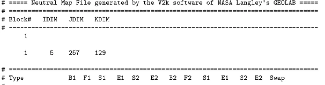
The utilityplot3d to aflr3converts a PLOT3D structured grid to an AFLR3-format hexahedral unstructured grid. The original structured grid must be 3D multiblock http://www.grc.nasa.gov/WWW/wind/valid/plot3d.html (no iblanking) with the file extension .p3d for formatted ASCII or the the file ex-tension.ufmtfor Fortran unformatted. Only one-to-one connectivity is allowed with this option (no patching or overset). The grid should contain no singular (degenerate) lines or points. A neutral map file with extension.nmfis also re-quired. This file gives boundary conditions and connectivity information. The .nmffile is described at http://geolab.larc.nasa.gov/Volume/Doc/nmf.htm. Note that the Type name in the .nmf file must correspond with one of
Fun3D’s BC types, plus it allows the Type one-to-one. If the Type is not recognized, you will get errors like:
This may be an invalid BC index.
An example .nmf file is shown here for a simple single-zone airfoil C-grid (5×257 ×129) with six exterior boundary conditions and one one-to-one
patch in the wake where the C-grid attaches to itself:
# ===== Neutral Map File generated by the V2k software of NASA Langley's GEOLAB ===== # ===================================================================================
# Block# IDIM JDIM KDIM
# ---1 1 5 257 129 # =================================================================================== # Type B1 F1 S1 E1 S2 E2 B2 F2 S1 E1 S2 E2 Swap #
---'tangency' 1 3 1 257 1 129 'tangency' 1 4 1 257 1 129 'farfield_extr' 1 5 1 129 1 5 'farfield_extr' 1 6 1 129 1 5 'one-to-one' 1 1 1 5 1 41 1 1 1 5 257 217 false 'viscous_solid' 1 1 1 5 41 217 'farfield_riem' 1 2 1 5 1 257 4.3.2 CGNS Grids
Fun3D is distributed with a utilitycgns to aflr3 that converts CGNS files http://cgns.sourceforge.net/ to AFLR3 grids. This utility will only be built if Fun3D is configured with a CGNS library, see section A.7.12. Only
the Unstructured type of CGNS files are supported. The following CGNS mixed element types are supported: PENTA 6(prisms),HEX 8(hexes),TETRA 4
(tets), and PYRA 5 (pyramids).
The CGNS file must includeElements tnodes for all boundary faces (type
QUAD 4orTRI 3) to refer to the corresponding boundary elements. Otherwise, the utility cannot recognize what boundaries are present because it currently identifies boundaries via these 2D element types. The cgns to aflr3 utility requires that the BC elements be listed either as a range or a sequential list.
It is also helpful to have separate element nodes for each boundary element of a given BC type. This way, it is easier to interpret the boundaries, i.e., body versus symmetry versus farfield. Visualization tools, such as Tecplot, can easily distinguish the various boundary condition groups as long as each group has its own node in the CGNS tree. Under BC t, cgns to aflr3 reads these BC names, but ignores additional boundary data (e.g., BCDataSet, BCData).
If the CGNS file is missing BCs (no BC t node), cgns to aflr3 still tries to construct the BCs based on the boundary face Elements tinformation. If these boundary element nodes have a name listed in Table 7, a .mapbc file will be written that contains the Fun3Dboundary condition numbers. If the
name is not recognized, you will see the message:
WARNING: BC type ... in CGNS file not recognized.
in which case you will need to fix it by by editing the .mapbc file manually. Always check the .mapbc file after the utility has run, to make sure that the BCs have all been interpreted and set correctly. If a translation problem is observed, you should edit the.mapbc file before running Fun3D.
Table 7: Boundary type mapping between CGNS and Fun3D.
CGNS FUN3D
BCSymmetryPlane 6661, 6662, or 6663 via prompt BCFarfield 5000 BCWallViscous 4000 BCWall 4000 BCWallInviscid 3000 BCOutflow 5026 BCTunnelOutflow 5026 BCInflow 5000 BCTunnelInflow 5000
5
Flow Solver,
nodet
This chapter covers what is required to run an initial flow solution, how to restart a flow solution, and how to specify what outputs the solver nodet
produces.
5.1
Flow Solver Execution
The grid and flow conditions are specified in the filefun3d.nml; see sectionB.4 for the file description. If you configuredFun3Dwithout MPI, the executable is namednodet. If you configuredFun3Dwith MPI, the executable is named
nodet mpi. Configuration and installation is explained in detail in section A. The executablenodet can be invoked directly from the command line,
nodet [fun3d options]
but the MPI version nodet mpi will need to be invoked within an MPI envi-ronment. The most common method is via
[MPI run command] [MPI options] nodet_mpi [fun3d options]
The details of the MPI run command and MPI options will depend on the MPI implementation. The MPI run command is commonly mpirun or mpiexec. The MPI options may contain the number of processors -np [n], a machine file -machinefile [file], or no local -nolocal. If a queuing system is used (e.g., PBS) this command will need to be run inside an interactive job or a script. See your MPI documentation or system administrator to learn the details of your particular environment.
If you have provided a grid with boundary conditions and fun3d.nml, you will then see the solver start to execute. If an unexpected termination happens during execution, especially during grid processing or the first iteration, you may need to set your shell limits to unlimited,
$ ulimit unlimited # for bash
$ unlimit # for c shell
A detailed description of the output files is given below.
5.2
Command Line Options
These options are specified after the executable. The majority of the command line options are functionality under development and there is work underway to migrate command line options to namelists. Namelists are the preferred input method. Command line options should be avoided unless they are the only way to activate the functionality you require. These commands are always preceded by -- (double minus). More than one option may appear on the
command line (each option proceeded by a -- ). You can see a listing of the available command line options in any of the codes in the Fun3D suite by
using the command line option --help after the executable name,
./nodet_mpi --help
The options are then listed in alphabetical order, along with a short de-scription and a list of any auxiliary parameters that might be needed, and then the code execution stops. Specific examples of the use of command line options are found throughout this, and later, chapters.
5.3
Output Files
These are the output files produced by the flow solver, nodet.
[project rootname].flow This file contains the binary restart infor-mation and is read by the solver for restart computations. See therestart read
namelist variable in section B.4.9 to control restart behavior.
[project rootname] hist.dat This file contains the convergence his-tory for the RMS residual, lift, drag, moments, and CPU time, as well as the individual pressure and viscous components of each force and moment. The file is in Tecplotformat. See sectionB.4.13for an improved method to track forces and moments.
[project rootname] subhist.dat For time accurate computations only. This file contains the sub-iteration convergence history for the RMS residuals. The file is in Tecplotformat.
[project rootname].forces This file contains a breakdown of all the forces and moments acting on each individual boundary group. The totals for the entire configuration are listed at the bottom. See section B.4.13 for an improved method to track forces and moments.
5.3.1 Flow Visualization
There are four basic categories of output: boundary data, sampling data (on entities such as planes, boxes and spheres), volumetric data, and slice data controlled by the namelists in Table 8.
Each namelist has a corresponding frequency variable, A positive frequency will cause the output to be generated every frequency time step/iteration. A negative frequency will cause output to be written only at the end of a run. A zero frequency (the default) with produce no output. See the corresponding namelist descriptions for details.
Table 8: Solver output types.
Type Namelist
domain boundaries &boundary output variables sectionB.4.21 domain volume &volume output variables sectionB.4.20 boundary slices &slice data sectionB.4.24 various geometries &sampling parameters and sectionB.4.23 and
&sampling output variables sectionB.4.22 point &sampling parameters and sectionB.4.23 and
&sampling output variables sectionB.4.22
5.3.2 Flow Visualization Output From Existing Solution
If a Fun3D flow solution already exists, visualization files by setting nsteps = 0in the &code run controlnamelist within the fun3d.nmlfile and setting the restart read variable to something other than ’off’. This will allow generation of visualization output without having to do additional timesteps or iterations.
6
Adjoint Solver,
dual
This section describes how to execute the adjoint solver,dual, directly. Typ-ically, dual is executed by scripts that manage the multiple steps required
for design optimization (section 8) or grid adaptation (section 7). However, it may be necessary to run dual directly to diagnose problems or gain expe-rience during setup including determining input parameters and termination strategies. Fun3D is configured to compile dual by default. While the
ad-joint method is available for most commonly used Fun3Dcapabilities, only a subset of Fun3D’s full capabilities are implemented in the adjoint solver.
6.1
Convergence of the Linear Adjoint Equations
The adjoint solution is dependent on the primal flow solution (and the con-vergence of the primal flow equations). While the primal solution may have converged enough to give acceptable force and moment results, the flow resid-uals might still be large, which can cause the adjoint solution scheme to di-verge. This divergence issue is most common in turbulent simulations. A divergent adjoint scheme can be improved in some circumstances with the
--outer loop krylov command line option. It is critical to run the flow solver and the adjoint solver with the same governing equations and bound-ary conditions.
The scaling of the adjoint residuals is different from the flow residuals and is dependent on the choice of the adjoint cost functions. The number of iterations steps and the residual tolerance stopping tolerancewill need to be adjusted, see section B.4.9. The sensitivities should converge at the same rate as your functions (i.e., lift), but an adjoint with some algebraic error may still provide reasonable sensitivities for design and grid adaptation.
6.2
Required Directory Hierarchy and Executing
dual
The executabledual can be invoked directly from the command line,
dual [fun3d options]
but the MPI version dual mpi will need to be invoked within an MPI envi-ronment. The most common method is via
[MPI run command] [MPI options] dual_mpi [fun3d options]
Any[fun3d options]provided tonodetthat control the flow solver residual
will also be required for the adjoint solver for a consistent adjoint solution and solution scheme. See the flow solver execution instructions for more details, section 5.1.
dual expects the cost function description ../rubber.data to be in the parent directory of the directory from which it is invoked. The input and flow restart files are shared with nodet in the directory ../Flow/. The flow solver must be run to completion, to provide a flow restart file, before dual
is invoked. See Table 9 for the required files and locations.
Table 9: Adjoint solverdual directory hierarchy.
Relative Path Description
../Flow/[project rootname].flow Primal flow solution (restart) ../Flow/fun3d.nml Main input namelist file
../rubber.data Description of the adjoint cost function
6.3
rubber.data
The minimum required information for running the adjoint (and grid adap-tation) is included below. See section 8.6.2 for complete details on including the information required for design. The reader for this file requires the ex-act number of header lines. Be very careful when editing this file. The cost function isclin this case. Available cost functions are discussed in section8.1.
######################################################################### ######################## Design Variable Information #################### ######################################################################### Global design variables (Mach number / angle of attack)
Index Active Value Lower Bound Upper Bound
Mach 0 0.1000000000000E+01 0.0000000000000E+00 0.5000000000000E+01 AOA 0 0.1000000000000E+01 0.0000000000000E+00 0.5000000000000E+01 Number of bodies
0
######################################################################### ############################ Function Information ####################### ######################################################################### Number of composite functions for design problem statement
1
######################################################################### Cost function (1) or constraint (2)
1
If constraint, lower and upper bounds
0.100000000000000 0.500000000000000
Number of components for function 1 1
Physical timestep interval where function is defined
1 1
Composite function weight, target, and power 1.0 0.0 1.0
0 cl 0.0 1.000 0.00000 1.00 Current value of function 1
0.000000000000000
Current derivatives of function wrt global design variables 0.000000000000000
0.000000000000000
6.4
Output Files
The adjoint solver will export visualization files in the same manner as the flow solver when requested, see section 5.3.1.
[project rootname].adjoint This file contains the binary restart in-formation and is read by the and adjoint solver for restart computations.
[project rootname] hist.tec This file contains the convergence his-tory for the RMS residual of the adjoint equations and CPU time. The file is in the same Tecplotformat as the flow solver produces. History information is truncated when the adjoint solver is restarted.
7
Grid Adaptation
Fun3D implements metric-based adaptation, where grid adaptation is
sepa-rated into two tasks. The first step is to construct a metric that describes the desired size and anisotropy of the adapted grid elements. The second step is to produce an adapted grid that is based on this metric.
Feature-based adaptation constructs the metric based on properties of the flow solution. Adjoint-based adaptation constructs the metric from the flow and adjoint solutions to reduce estimated errors in a specified output function. The namelist&adapt metric construction(sectionB.4.28) for specifying de-tails of the metric.
Fun3D supports a number of grid adaptation libraries. The namelist
&adapt mechanics (section B.4.29) specifies the grid adaptation library and its options. The refine library is distributed and installed with Fun3D by
default.
7.1
Geometry Specification and Grid Freezing for
re-fine
When adapting a grid with refine, all boundary faces must be specified as
frozen or a geometry definition mush be provided via FAUXGeom. Use the default patch lumping=’none’ in the &raw grid namelist, as lumping will change boundary patch indexes making it more difficult to specify geometry.
7.1.1 No geometry, where the surface nodes are frozen.
refinecannot preserve the high aspect ratio structures within viscous layers,
and so viscous layers must be frozen for a specified distance away from the surface to maintain grid quality. This is invoked with the adapt freezebl
command within the&adaptation mechanicsnamelist, see sectionB.4.29for more details.
Additionally, specific surfaces that do not have a viscous boundary condi-tion can be frozen by listing the surface numbers (one per line) in a file named
[project rootname].freeze. For example,[project rootname].freezethat contains
5 7
will freeze points on boundary patches 5 and 7. This is also useful for boundary surfaces that do not have an analytical definition handled by FAUXGeom.
7.1.2 FAUXGeom for Planar Boundaries
For viscous problems, where the mesh on the complex geometry of the body is frozen, FAUXGeom can be used to provide an analytical definition of the farfield boundary surfaces. This allows adaptation to occur on the planar sur-faces of the mesh, even when the boundary layer mesh is frozen. This is a particularly important capability for symmetry planes. At present, FAUX-Geom can only handle planar surfaces.
FAUXGeom reads the file faux input. Here is an example file:
4 5 xplane -5.0 3 yplane -1.0 1 zplane 1.0 16 general_plane 2.0 0.707 0.707 0.0
The first line is how many faux surfaces are being defined. The subsequent lines have a face number, type of face, and a distance associated with the particular geometry. In this example, the first faux face defined corresponds to surface 5 in the mesh and is a x = −5.0 constant plane. Faux faces are similarly defined for the z and y planes of surfaces 3 and 1. Surface 16 is a plane perpendicular to a (0.707,0.707,0.0) normal that is located 2.0 away from the origin in the direction of the normal; the plane passes through the point (1.414,1.414,0.0).
7.2
Performing Feature-Based Adaptation
The &adapt metric constructionvariable adapt feature scalar form de-fines the operator that is applied to the adapt feature scalar key to com-pute an adaptation intensity. This intensity is raised to the adapt exponent
power to produce a scaling of an isotropic element size estimate on the cur-rent grid. The anisotropy of the metric is introduced by the Hessian of the
adapt hessian key variable.
Set restart read=’on’ in section B.4.9 to read the flow solution. Run
nodet with the --adaptcommand line option in the directory with the flow restart. The result will be a new grid and interpolated solution file with the adapt project project name. After adaptation, the flow solver can now be restarted with this new grid and interpolated solution by changing the
project rootname.
7.3
Performing Adjoint-Based Adaptation
Adjoint-based adaptation requires that a flow solution be calculated in the
See section 6 for more information on obtaining an adjoint solution. The adjoint solution is based on the functional defined in rubber.data and this is the same functional targeted for grid adaptation.
Adaptation is performed by executing dual with the command line
op-tions --rad --adapt. The adjoint solver reads the fun3d.nml in the ../Flow
directory), so this is the place to specify &adapt metric construction and
&adapt mechanics options. The freeze and FAUXGeom files are read in the current directory, Adjoint.
The result will be a new grid and interpolated solution restart file in the ../Flowdirectory and an interpolated adjoint restart in theAdjointdirectory. The project name of these new files is adapt project.
7.4
Scripting Grid Adaptation
TheFun3Dinstallation includes thef3dscript. To find the other components of the Fun3D suite, the f3d script expects to be in the bin directory of the
Fun3Dinstallation. Don’t copy or linkf3dfrom thebindirectory. The input file case specifics is described in section7.4.1.
Execute thef3dscript in a directory that contains all of the the input files (e.g., grid, fun3d.nml, case specifics). The script will create the required
Flowand Adjointdirectories to run the case. It has the following commands,
usage: f3d <command> <command> description ---
---start Start adaptation
view Echo a single snapshot of stdout
watch Watch the result of view
shutdown Kill all running fun3d and ruby processes
clean Remove output and sub directories
The command start begins adaptation by launching a background job. The commands view and watch allow the adaptation progress to be monitored. (Use Ctrl-C to escape the watch command.) The shutdown command kills all ruby (f3d) and Fun3D jobs. The clean command removes the Flow and
Adjointsubdirectories and the output log file.
7.4.1 Input File case specifics for f3d Script
Thef3dscript has one input file, namedcase specifics. Here is an example
root_project ''
number_of_processors 2 mpirun_command 'mpiexec'
first_iteration 1 last_iteration 10
# Any text after a number sign is a comment.
where the defaults are listed. Adaptation will be performed from the first grid adaptation iteration 1 to the last grid adaptation iteration 10. The string in quotes next to root project is the project root name. A two digit iteration number will be appended to it. The project name for the first adaptation will be [root project]01 and the last will be [root project]10. All the files required to run nodetand dual should be provided in the current directory
and the grid filename should include the root project name and iteration num-ber, [root project]01. Flow and Adjoint subdirectories are created by the script during execution, and the input files are placed in their correct location by the script.
Command line options can be passed to the codes via,
all_cl ' ' flo_cl ' ' adj_cl ' ' rad_cl ' '
where all cl is provided to all codes, flo cl is provided to nodet, adj cl
is provided todual during the adjoint solve, andrad cl is provided todual
during error estimation and adaptation. For example, the line
adj_cl ' --outer_loop_krylov '
turns on Krylov projection wrapping to stabilize the adjoint solve.
The main input file fun3d.nml provided in the current directory can be modified by the following commands
all_nl['variable']= value flo_nl['variable']= value adj_nl['variable']= value rad_nl['variable']= value
where all nl changes fun3d.nmlfor all codes, flo nl for nodet, adj nl for
dual during the adjoint solve, and rad nl for dual during error estimation
and adaptation. An example is
adj_nl['steps']=500
adj_nl['stopping_tolerance']=1.0e-12
where the termination criteria of the adjoint solver can be specified separately than the flow solver.
The case specificsis actually executable Ruby code. This allows values to be computed or conditionally executed, but also require nested quotes for character strings,
rad_nl['adapt_complexity'] = 5000*iteration number_of_processors 128 if (iteration>5) all_nl['flux_construction'] = "'vanleer'"