Capital Flows in the Norwegian Mutual Fund Market

(1)

Capital Flows in the Norwegian Mutual

Fund Market

Thomas Hansen

Lars Kristian Steffensen

Industrial Economics and Technology Management

Supervisor: Peter Molnar, IØT

Department of Industrial Economics and Technology Management Submission date: June 2013

(2)

(3)

(4)

(5)

(6)

(7)

Preface

This master’s thesis is written during the spring of 2013 at the Norwegian Univer-sity of Science and Technology (NTNU). It marks the end of our Master of Science degree in Industrial Economics and Technology Management. Our economic spe-cialization is within the field of Financial Engineering. First and foremost, we would like to thank our advisor Peter Molnar for his contributions. His guidance, relentless encouragement and constructive criticism have been greatly appreciated. We would also like to thank Caroline Sesvold Tørring at the Norwegian Fund and Asset Management Association (VFF) and Truls Evensen at Oslo Stock Exchange for generously providing us with data.

(8)

(9)

Sammendrag

Denne oppgaven undersøker m˚anedlige pengestrømmer inn og ut av norske fond.

Datasettet best˚ar av aksje-, obligasjon- og pengemarkedsfond registrert p˚a Oslo

Børs i løpet av perioden 2006–2012. Oppgavens m˚al er ˚a identifisere

sammenhen-ger mellom disse pengestrømmene, b˚ade aggregerte pengestrømmer og individuelle

pengestrømmer for hvert fond, og en rekke forklaringsvariabler. Individuelle og

in-stitusjonelle investorer studeres b˚ade sammen og hver for seg. Resultatene tyder

p˚a at individuelle investorer er mer tilbøyelige til ˚a fokusere p˚a tidligere

prestasjo-ner enn institusjonelle investorer. I tillegg, innstrømninger til aksjefond forklares langt lettere av relative avkastninger enn utstrømninger fra aksjefond uavhengig av investortype. Spesifikt finner vi at innstrømninger er større for aksjefond som har utkonkurrert andre aksjefond i fortiden. Dette forholdet er mye sterkere i opp-gangstider og svakere for volatile aksjefond.

(10)

(11)

Abstract

This paper investigates monthly capital inflows, outflows and net flows for Norwe-gian mutual funds. The data set contains equity, bond, and money market funds registered at some point in the period 2006–2012 on Oslo Stock Exchange (OSE). The goal of the study is to identify relationships between these flows, both aggre-gated flows and flows for individual funds, and a range of explanatory variables. Retail and institutional investor flows are studied both separately and overall. The results indicate that retail investors, when making investment decisions, are more likely to focus on past performance than institutional investors. Moreover, equity inflows are more easily explained by past relative returns than equity outflows re-gardless of investor type. Specifically, inflows are larger for equity funds that have outperformed other equity funds in the past. This relationship is much stronger in bull markets and weaker for volatile equity funds.

(12)

(13)

1 Introduction

The purpose of this paper is to investigate capital flows to and from Norwegian mutual funds. Our data consist of equity, bond, and money market funds registered, at some point, on Oslo Stock Exchange (OSE) in the period January 2006 to December 2012. We study a set of explanatory variables potentially related to these fund flows. This may be of general economic interest as a study of basic investor behavior, and it may be of specific economic interest for fund managers and other parties involved in the mutual fund industry. The main question posed can be formulated as follows: What are the determinants of capital flows in the Norwegian fund industry?

In answering this type of question, most papers only investigate equity funds which often are readily available. We, however, have access to bond and money market fund flows as well. Furthermore, a lot of research is limited to just approx-imated net flows because raw flow data is not available. We, on the other hand, have access to monthly inflows and outflows directly. Therefore we can investigate flows on a deeper level than just net flows - we can isolate inflows and outflows.

Also, most papers treat investors as one homogeneous group. However, it would

be interesting to study different types of investors separately. Our data set is

divided into Norwegian retail and institutional investors. There may be significant differences in the level of sophistication and purpose among these investors. As an example, retail investors may be less educated, in general, compared to professional institutional investors. This may again lead to different allocation decisions and preferences.

Our research is is split up into two parts. Firstly, we investigate aggregated flows for each of the fund categories – equity, bond and money market funds. That is, we add up inflows, outflows and net flows for all funds in each category. The method used is multiple linear regression. The flows are the independent variables and relevant market variables are the explanatory variables.

The inspiration for this part of our study comes primarily from two sources. Ederington and Golubeva (2011) investigate a broad set of market variables to describe the capital flows to equity, bond and money market mutual funds in the US. Gallefoss et al. (2011) look specifically at capital flows in the Norwegian equity fund market. The idea is to introduce the broad perspective of Ederington and Golubeva (2011) to the Norwegian mutual fund market while including specific features of the Norwegian market used by Gallefoss et al. (2011).

Secondly, we investigate individual flows for equity funds. Now, individual

equity fund inflows, outflows and net flows are the dependent variables and fund-specific variables are the explanatory variables. The method used for this part of our research is Fixed Effects panel data regression. The inspiration comes from

several different sources. Clifford et al. (2011) isolate retail and institutional

investors and find significant differences between the two investor groups. Shu et al. (2002) and Huang et al. (2011) utilize similar approaches and find corresponding results. However, this is yet to be done in the Norwegian market.

To summarize, we first describe aggregated flows to and from each fund cate-gory using market variables, before diving deeper into the equity fund market using

(16)

individual fund flows and fund-specific variables. This will provide us with two dif-ferent perspectives on the Norwegian mutual fund industry: The broad, overall developments and trends in the market versus the direct competition between spe-cific funds.

As mentioned, we utilize multiple linear regression and panel data regression. This provides results in the form of statistically significant or non-significant co-efficients estimates. A significant coefficient estimate implies a linear relationship between the explanatory variable and the flow under study. A positive relation-ship implies a tendency to move together, whereas a negative relationrelation-ship implies a tendency to move in opposite directions, all else being equal. To ensure robust results, we use different measures of past performance and flow. The inspiration for this approach comes primarily from Li et al. (2013) and Spiegel and Zhang (2013). This will help to ensure that our results are not simply consequences of misspecifications.

It is also appropriate to comment on a few limitations of this paper. Some of these are deliberate choices whereas others are consequences of data availability and/or quality. Firstly, this paper does not look into hybrid funds as results are expected to be vague and camouflaged by the presence of both equity and bond components. Investigating the three mentioned mutual fund categories being eq-uity, bond and money market funds is considered sufficient to address the question of interest.

Also, the available flows are, as mentioned, obtained at a monthly basis from January 2006 to December 2012. This monthly interval therefore becomes the observation interval for all explanatory variables as well, even if some of these have higher observation frequencies.

The period under investigation also includes the recent financial crisis. Even though the Norwegian economy managed quite well through this difficult period, no one was left unmarked. This may affect the relationships and estimates found. We also want to mention that broker fees are not included. Broker fees are more or less constant for the vast majority of funds, and the Fixed Effects panel data regression method controls for such time-invariant variables. Thus, the exclusion of broker fees will not affect the remaining variables.

(17)

2 LITERATURE REVIEW

2 Literature Review

Some papers with interesting perspectives on the area of study are presented below. A lot of research finds more or less corresponding results, consequently only enough papers are presented to cover the main findings.

Ederington and Golubeva (2011) investigate flows from a set of open-ended mutual funds registered in the US. They use a relatively large amount of variables that have been suggested to have predictive power about future risk and return. In addition to actual past risk and return, these variables are used to explain observed capital flows. Furthermore, they are not limited to equity funds, but also include bond and money market funds. Their findings suggest that a wide range of macroeconomic variables are related to mutual fund flows.

Gallefoss et al. (2011), investigate net flows to a set of open-ended equity mutual funds registered on Oslo Stock Exchange (OSE). They limit their research to equity

funds with domestic investments. The paper looks at past returns, fund size,

fund fees, and other microeconomic variables to explain observed flows. They

also investigated a set of macroeconomic variables including the oil price and the USD/NOK exchange rate - both presumably highly relevant for the Norwegian economy. The former is found to be significant in their study, but the latter is not. These variables are also included in our study.

Ivkovi´c and Weisbenner (2009) study capital flows to and from mutual funds in

the US. They find that inflows are driven mainly by relative performance - more precisely, a mutual fund’s one-year performance relative to other comparable risk funds. In other words, new money chases the best performers. Outflows, however, are mainly driven by absolute performance. Their main reflection of interest to us is that inflows and outflows may have significantly different drivers. Consequently they should be studied separately, as well as unified, to achieve a more complete description of the flows.

Ederington and Golubeva (2009) further motivates the decision to look at in-flows and outin-flows separately. They do find that increased volatility is negatively correlated with net flows, but, more interestingly, inflows as well as outflows in-crease with inin-creased volatility. This indicates that volatile times in general lead to a higher total activity level. Increased returns, on the other hand, seem to affect inflows to a much stronger degree than outflows. Summarizing this, inflows seem to be driven by returns and risk while outflows seem to be driven mainly by risk. The reasonable chance to make a high return may lead you into the market while fear drives you out.

The main results of Sirri and Tufano (1998) are also related to the dispropor-tionality between how inflows and outflows react to fund performance. They study equity funds in America, and find that inflows are much more sensitive to past per-formance than outflows. In other words, investors seem to flock to past winners, but fail to flee from past losers.

Jank (2012) is one of the few recent papers that include a wide range of macroe-conomic variables to explain the correlation between return and fund flow. The paper concludes that macroeconomic news are highly relevant for both fund flows

(18)

and market returns, and therefore may explain the high correlation found between these two measures. In other words, flows and returns are both forward looking and are a result of predicted economic activity. So, as these macroeconomic vari-ables are correlated with future returns, they are also correlated with fund flows. A limitation of this study is that it only utilizes data from America and it only includes equity funds.

Kim (2010) brings an interesting view of volatility to the topic. The paper finds that flows are less sensitive to high performance under volatile conditions. In addition, investors mainly focus on past performance relative to competitors. This implies that the high performance effect is a relative issue. This study uses only equity funds, but the general idea that flow sensitivity to high returns is very much dependent on market volatility might be valid also for bond and money market funds. Variables reflecting the volatility level should therefore be included in various forms.

Clifford et al. (2011) investigate recent equity fund flows and find that most investors chase past performance to a high degree. The interesting part, however, is that they further find that investors do this with little regard to risk - somewhat contradictory of what Kim (2010) found. In other words, this study seems to indicate that investors are somewhat less rational than Kim (2010) found. One advantage of Clifford et al. (2011) is that they separate inflows and outflows as previously discussed. They may therefore have a more precise picture of inflows than Kim (2010). We will investigate this relationship in more detail.

Furthermore, Clifford et al. (2011) isolate retail and institutional investors. They find that institutional investors do not chase past performance to the same degree as retail investors. Additionally, retail investors chase idiosyncratic risk - that is, they focus on returns and do not evaluate the underlying risk. These findings indicate that institutional investors are somewhat more sophisticated in their investment decisions than retail investors. Intuitively, this makes sense as institutional investors are likely to be professional staff. Anyhow, Clifford et al. (2011) find signs of clear behavioral bias. Behavioral differences between retail and institutional investors are also part of our investigation.

Shu et al. (2002) investigate flows in and out of equity funds in Taiwan. They conclude that small-amount investors have a tendency to chase past performance and be quick to capitalize on gains. Large-amount investors, on the other hand, are not notably affected by short-term performance. Intuitively, retail investors are likely to be small-amount investors, and institutional investors are likely to be large-amount investors. Under this assumption, this research would be in line with Clifford et al. (2011).

Jank & Wedow (2012) use a sample of German registered equity funds. Their main finding of interest is that investors have a tendency to sell both so-called win-ners and losers. That is, funds performing very well or very poorly both experience relatively large outflows. Presumably, funds performing very well also experience large inflows. Additionally, funds from large fund families in general experience both higher sales and redemption rates. Multiple explanations may justify this observation - for example easily available information to act upon.

(19)

2 LITERATURE REVIEW

Among other things, Huang et al. (2011) investigate the relationship between flows and past returns for retail versus institutional funds in the US. That is, to what extent fund flows react to past performance. They find that retail investors are less concerned with idiosyncratic volatility than institutional investors. Low volatility might imply that past returns are more likely to be repeated, whereas high volatility makes the future much more uncertain. Following this argumentation, fund flows should be less sensitive to returns from volatile funds. Huang et al. (2011) conclude that institutional investors drive this dampening effect and underline the importance of investor heterogeneity.

Li et al. (2013) is a recent study of the Chinese equity fund market. They investigate equity fund flows through a range of fund-specific variables, very much like we do for individual flows. They infer highly significant results for various measures of past returns and control variables such as TNA and age. In particular, they find that net flows are much more sensitive to returns in bull markets than bear markets. Possibly, the uncertainty and volatility of bear markets might explain this finding - performance persistence is less likely to occur. We bring with us this finding, in addition to their approach to include various measures of past performance as a robustness check. Additionally, we also investigate inflows and outflows separately.

Finally, a note on fund flow measures is appropriate. Spiegel and Zhang (2013) bring an interesting view on the topic of flow measures. Usually, raw flows are not used exclusively in the studies above for two reasons. Firstly, large funds may be expected to have larger inflows and outflows than small funds. The reason for this may be that large funds, in general, are more well-known and easier to gather information about. Secondly, the mutual fund industry overall has grown rapidly the last decades. This implies that larger flows are expected now than before. Because of this, relative flow measures are often used instead of raw flows. Relative flows are typically raw flows divided by total net assets (TNA) of the same fund, as in Sirri and Tufano (1998). This will to some extent correct for fund size bias. However, Spiegel and Zhang (2013) argue that also this measure is far from ideal. Instead they propose a measure of change in market share as being more appropriate to infer relationships between flows and past returns. We use their formula for change in market share as an additional measure of net flow and include it in our study.

(20)

(21)

3 DATA

3 Data

By the end of 2012, the Total Net Assets (TNA) in the Norwegian fund market

reached an all time high of 558 billion Norwegian Kroner (NOK)1_{. The fund market}

is dominated by three main categories of funds, namely equity funds, bond funds and money market funds.

Table 1: Breakdown of TNA in the Norwegian fund market (2012) (a)TNA allocated among fund categories

Fund category Market share

Equity funds 49%

Bond funds 24%

Money market funds 16%

Other funds 11%

(b) TNA allocated among investors

Investor category Market share

Institutional investors 57%

Retail investors 29%

Foreign investors 13%

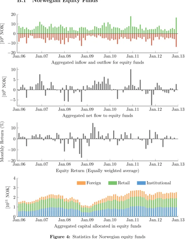
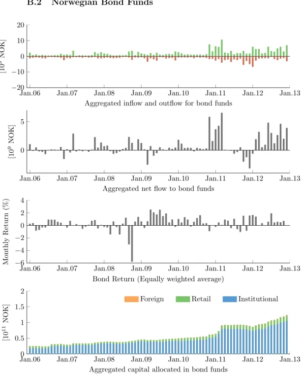
As seen from Table 1b, institutional investors dominate the market. This is partic-ularly evident for bond and money market funds, whereas capital in equity funds is more evenly divided between institutional, retail and foreign investors. Foreign investors will not be studied separately as the number of observations is limited. Additionally, foreign investors constitute a mix of the two main investor groups, retail and institutional investors. Therefore results will be difficult to interpret. However, when results are presented for investors overall, foreign investors are in-cluded.

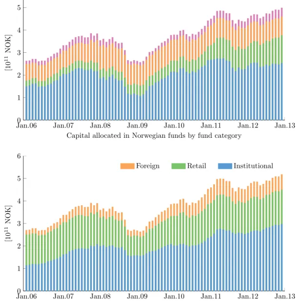
Jan.060 Jan.07 Jan.08 Jan.09 Jan.10 Jan.11 Jan.12 Jan.13

2 4 6 [10 11 NOK]

Other Money Market Bond Equity

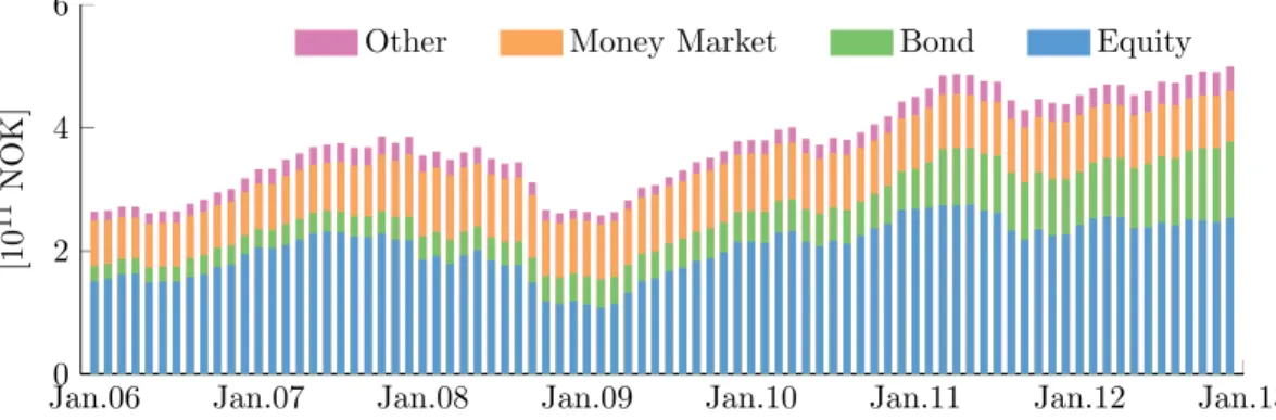
Figure 1: Capital allocated in Norwegian funds by fund category

The capital allocated in Norwegian funds since the financial crisis has nearly dou-bled, largely driven by increased investments in equity and bond funds as seen from

1_{According to the Norwegian Mutual Fund Association (VFF). The graph given in Figure}

1 only includes funds registered on the Oslo Stock Exchange (OSE). Funds held by domestic investors on other stock exchanges are therefore not included.

(22)

Figure 1. A more detailed breakdown of the Norwegian fund market with capital flows and returns is given in Appendix B.

In the following, we present the data and sources used in our various regression models. To analyze how different return measures affect the flow sensitivity, we

have collected daily Net Asset Values (NAV)2 _{and flow data for funds.}

3.1 Data Sources

3.1.1 Fund returns

Oslo Stock Exchange (OSE) has provided daily NAVs and dividend payments for all funds registered on OSE at some point during the 7-year period from 2006 to 2012.

3.1.2 Fund flows

The Norwegian Fund and Asset Management Association (VFF) publishes monthly spreadsheets of fund flow statistics. We have written a VBA macro which col-lects the monthly observations and constructs flow time series for each fund. The members of VFF include the majority of large-sized brokers operating in Norway. Each broker is required to report measures such as inflows, outflows, reinvested dividends, number of customers and total net assets differentiated between three investor categories:

• Norwegian retail investors

• Norwegian institutional investors

• Foreign investors (Retail and institutional)

VFF also divide the funds into six different categories depending on their invest-ments and risk exposure:

• Equity Funds

• Hybrid Funds

• Money Market Funds

• Bond Funds

• Hedge Funds/Other Funds

• Other High-Yield Funds

2_{The Net Asset Value is defined as the total net assets divided by the number of outstanding}

(23)

3 DATA

In this paper, as discussed previously, we focus on equity, bond and money market funds. This excludes hedge funds, hybrid funds and other funds which do not meet the criteria of the three categories. All member funds traded in the period 2006-2012 are included, and the data is thus free of survivorship bias.

For the aggregated regressions, we use the entire set of funds reported by VFF. This includes a total of 435 equity funds, 58 money market funds and 87 bond funds. For the panel data regressions, we introduce certain requirements due to the longitudinal nature of our data. Specifically, there are effects of fund flows which are “smoothened” out by aggregation, but are present at an individual level. Three assumptions are made in section 3.4 which exclude certain observations in the panel regression (individual flow) data set. As only equity funds have a sufficient number of observations after introducing these requirements, we only run panel data regression for 245 equity funds.

3.2 Variables - Aggregated Flows

To study aggregated flows we utilize multiple linear regression. As mentioned in the introduction, the set of market variables used in this paper is inspired by two main sources. Ederington and Golubeva (2011) utilized a wide range of variables including aggregated returns, volatility measures like VIX and MOVE, stock mar-ket trend, and different spreads especially relevant for the mutual fund marmar-ket. Some of these have been utilized directly in this paper, whereas others have been modified to more closely reflect the Norwegian market. Gallefoss et al. (2011) investigated factors likely to be relevant for the Norwegian market in particular. Example of this are the price of Brent Crude Oil and USD/NOK exchange rate.

In addition to these variables, several potentially relevant factors are inves-tigated. The three-month NIBOR is included to reflect the general short term interest level in the Norwegian market. The one-month historical volatility on the OSEAX (Oslo Stock Exchange All Share Index) is intended to more closely reflect the domestic volatility.

All in all, we have a total of 83 monthly observations for all fund and investor categories. This includes all months from February 2006 - December 2012 except January 2006. Observations from January 2006 are omitted from the regression as we do not have data for the total net assets of December 2005 needed to calculate relative flows.

3.2.1 Dependent variables

We utilize three different flow measures to study aggregated fund flows. We include

raw flows,F. In addition, we include a fractional flow specification, ˆF in accordance

with conventions in literature where we divide the flow to the specific investor category by the capital of that specific investor category the previous month. This can be interpreted as percentage growth in assets beyond return and reinvested dividends. Spiegel and Zhang (2013) suggests that this fractional specification is misspecified and propose change in market shares as a more robust measure of net flows. This market share measure has no directly equivalent measure for

(24)

inflows and outflows, and we apply the change in market share, ˜F, only for net flows. For inflows and outflows, we divide the inflows by the total capital of all fund categories in the specific investor category to achieve a related measure. The various flow measures are expressed mathematically below.

C={Retail investors,Institutional investors,All investors}

D={Equity Funds, Money Market Funds,Bond Funds}

ˆ

D={Equity Funds, Money Market Funds,Bond Funds - active at timet}

Inflowc_d,t= Aggregated inflow for fund categorydfor investor categoryc

Outflowc_d,t= Aggregated outflow for fund categorydfor investor categoryc

Net flowc_d,t= Aggregated net flow for fund categorydfor investor categoryc

TNAc_d,t= Total Net Assets of fund categorydfor investor category c

Aggregated flows are reported in 106 NOK and TNA are reported in 103NOK. All

investors is the sum of retail, institutional and foreign investors.

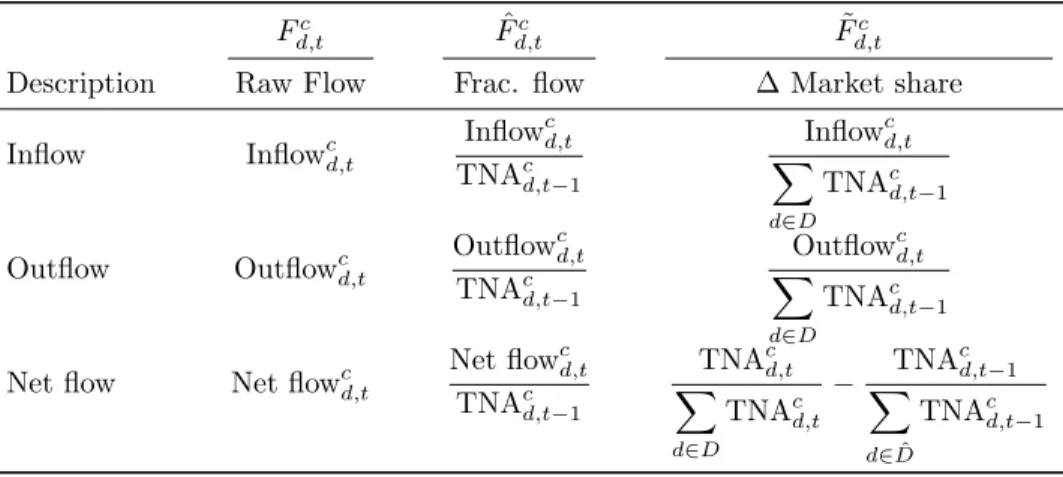
Table 2: Dependent variables used for aggregated flows

F_d,tc Fˆ_d,tc F˜_d,tc

Description Raw Flow Frac. flow ∆ Market share

Inflow Inflowc_d,t Inflow

c d,t TNAcd,t−1 Inflowc_d,t X d∈D TNAc_d,t₋₁

Outflow Outflowc_d,t Outflow

c d,t TNAcd,t−1 Outflowc_d,t X d∈D TNAc_d,t₋₁

Net flow Net flowc_d,t Net flow

c d,t TNAcd,t−1 TNAc_d,t X d∈D TNAc_d,t − TNAc_d,t₋₁ X d∈Dˆ TNAc_d,t₋₁ 3.2.2 Independent Variables Returns

Dividend-adjusted returns on individual funds are calculated from NAVs at the beginning and end of specified time periods. The returns reported here are one-year returns. Equally weighted average returns for each fund category are then calculated on the basis of these returns. All funds registered at some point in the period 2006–2012 are included.

Return on Equity Funds: r¯_teq

(25)

3 DATA

Return on Money Market Funds: r¯mo t

Equally weighted average return of money market funds over the interval

[t−11, t].

Return on Bond Funds: r¯bo t

Equally weighted average return of bond funds over the interval [t−11, t].

Volatility measures

Volatility on OSEAX: σose t

The volatility on the OSEAX is calculated as a one-month volatility. The OS-EAX consists of all shares registered on the exchange. This measure may give a domestic and precise estimate of stock market volatility in the Norwegian market.

Percentage change in historical volatility on OSEAX: %∆σose t

The percentage change in historical volatility from montht−1 tot. Changes

in volatility may be even more relevant than the general volatility level as investors are likely to react to changes in market conditions.

Other variables NIBOR: nibt

The 3-month NIBOR, the Norwegian Interbank Offered Rate, is intended to reflect the general interest level for unsecured money market lending which should be particularly relevant for bond and money market funds.

Oil Price: roil t

The oil price (Brent Crude) is a natural measure of the state of the Norwegian economy. It affects the Norwegian business environment to a very high degree and is therefore included as a possible explanatory variable.

Exchange Rate: r_tex

The exchange rate relates to purchasing power in Norwegian market and may therefore be relevant for investment decisions.

Volatility measures and other variables are originally gathered from EcoWin Reuters and then adapted to meet our specific needs.

(26)

3.3 Variables - Individual Equity Flows

In the panel data regressions, we only use fund-specific variables. We introduce two different measures of excess return. One is a simple excess return, calculated

as ri−r¯i which is just the return of the fund subtracted by the average return of

all stock funds registered on OSE over the interval [t−11, t].

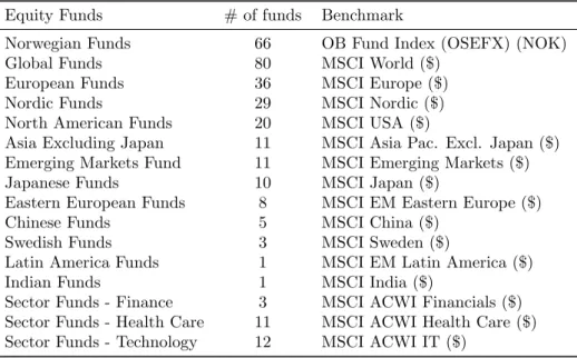
We also find a risk-adjusted excess return for each fund,αi,t, by applying the

Capital Asset Pricing Model (CAPM) with daily return observations over the

inter-val [t−11, t]. When this return measure is used, funds are separated into

subcate-gories with a proper benchmark specified for each subcategory. These benchmarks are listed in Appendix A.

3.3.1 Dependent variables

Three flow measures corresponding to the ones used for aggregated flows are used.

We apply a raw flow measure, F, a fractional flow specification ˆF, and a measure

equivalent to change in market share for net flows ˜F. Individual raw flows are

reported in 103 NOK. Mathematical formulations are given below.

C={Retail investors,Institutional investors,All investors}

I={Set of equity funds}

ˆ

I={Set of equity funds active at timet}

Inflowc_i,t= Inflow for fundifor investor categoryc

Outflowc_i,t= Outflow for fundifor investor categoryc

Net flowc_i,t= Net flow for fundifor investor categoryc

TNAi,t= Total net assets of fundifor investor categoryc

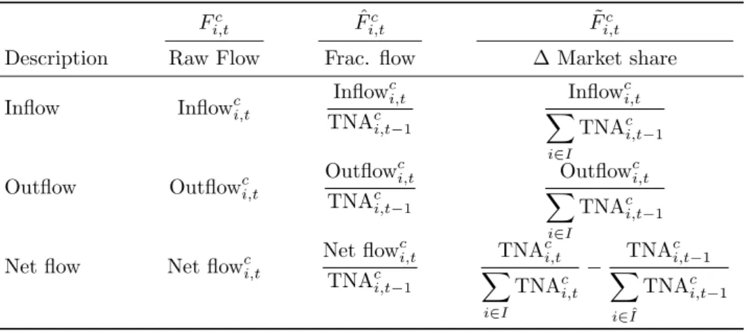
Table 3: Dependent variables used for individual equity flows

Fc

i,t Fˆi,tc F˜i,tc

Description Raw Flow Frac. flow ∆ Market share

Inflow Inflowci,t

Inflowc_i,t TNAc_i,t₋₁ Inflowc_i,t X i∈I TNAci,t−1

Outflow Outflowc_i,t Outflow

c i,t TNAc_i,t₋₁ Outflowc_i,t X i∈I TNAci,t−1

Net flow Net flowc_i,t Net flow

c i,t TNAci,t−1 TNAc_i,t X i∈I TNAc_i,t − TNAc_i,t₋₁ X i∈Iˆ TNAc_i,t₋₁

(27)

3 DATA

3.3.2 Independent variables

One year historical excess return of fund: rˆi,t

Excess return of the fund, eitherαi,torri,t−r¯i,t, over the interval [t−11, t].

This measure of past performance is included to explain why investors choose one equity fund over another.

Excess return multiplied by idiosyncratic risk: ˆri,tσ[i,t]

The idiosyncratic volatility, calculated from the residuals of CAPM over the

interval [t−11, t], is multiplied by the excess return measure to investigate

how the flow sensitivity to past returns is affected by fund-specific risk. The risk level of a fund may affect how investors perceive past performance.

Excess return multiplied by market indicator: ˆri,tindi,t

The market indicator variable,ind, takes a value of 1 if OSEFX (Oslo Stock

Exchange Mutual Fund Index) has a positive return over the interval [t−11, t],

and zero otherwise. As the idiosyncratic volatility, it is multiplied by the excess return measure. This approach will decompose the excess return and tell us if flows react differently to returns depending on the state of the general stock fund market.

Control variables

Age: log (agei,t)

This is the logarithm of the age of the fund measured in months at timet.

Capital of fund: log (T N Ac i,t)

This is the logarithm of the TNA of the fund at timet for investor category

c.

Number of customers for fund: log (cust.c i,t)

This is the logarithm of the number of customers of the fund at time t for

(28)

3.4 Data Requirements for Individual Equity Flows

In this section we introduce three requirements for individual equity flows.

Requirement 1.

Number of monthly flow observations≥12 (1)

Requirement 2.

Average number of institutional customers≥ 20

Average number of retail customers≥100

Average number of total customers≥ 20

(2)

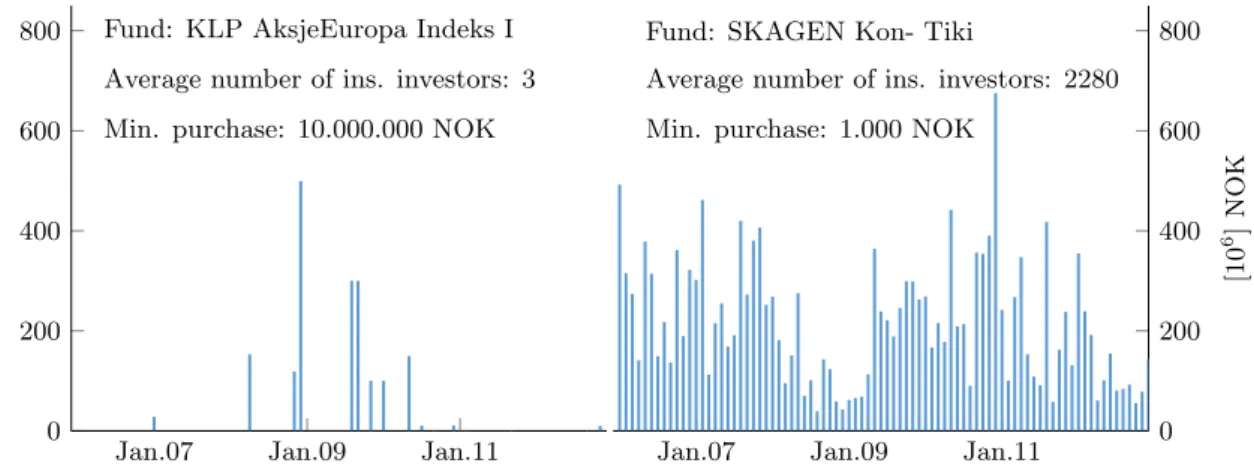
The rationale behind these assumptions is that small funds with few customers usually operate with high fees which results in very dispersed flows with many monthly observations of zero flow. In an attempt to capture funds which are openly traded, we introduce a minimum requirement to the average number of customers of the specific investor category of the fund. Note that the requirements given in (2) are set separately for each investor category. A fund which does not satisfy the requirement of institutional investors, could still be included in the retail investor category if it satisfies the requirements of number of retail investors. An illustration of our approach is given in Figure 2 below.

Jan.07 Jan.09 Jan.11 0

200 400 600

800 Fund: KLP AksjeEuropa Indeks I Average number of ins. investors: 3 Min. purchase: 10.000.000 NOK

[10

6 ]

NOK

Jan.07 Jan.09 Jan.11 0

200 400 600 800 Fund: SKAGEN Kon- Tiki

Average number of ins. investors: 2280 Min. purchase: 1.000 NOK

[10

6 ]

NOK

Figure 2: Comparison between the inflow from institutional investors to the funds KLP AksjeEuropa Indeks and Skagen Kon-Tiki. With the requirement of a mini-mum number of average institutional customers, the first fund is excluded.

(29)

3 DATA

Requirement 3.

The capital of liquidated funds are not included as outflows from funds. The

liquidation of a fund is often a decision made by the management, and not its investors. The liquidation of a fund’s assets is therefore not considered an outflow of the type we want to describe.

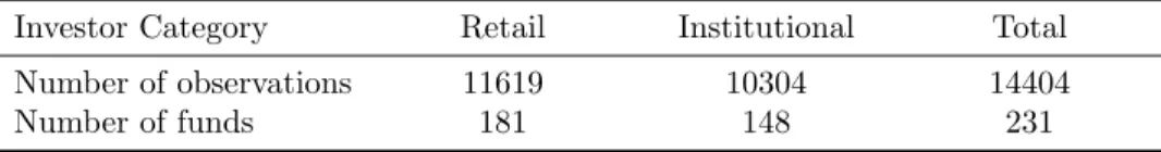
With these data requirements, the initial sample of 550 funds is reduced to:

Table 4: Sample statistics: Individual equity flows

Investor Category Retail Institutional Total

Number of observations 11619 10304 14404

(30)

(31)

4 METHODOLOGY

4 Methodology

Mutual fund flows are commonly investigated on an aggregated level. The advan-tage of aggregated data is that it is relatively straight forward to analyze. Ag-gregation smoothens out the noise which is often observed at an individual level. However, this also ignores individual differences caused by fund-specific charac-teristics such as relative performance and idiosyncratic volatility. Additionally, aggregation involves a substantial decrease in the number of observations, which makes statistical inference more difficult.

Some recent papers study mutual fund flows on fund-level, including Spiegel and Zhang (2013), Huang et al. (2011) and Li et al. (2013). As opposed to aggregated fund flows which are usually investigated by multiple linear regression, these papers utilize panel data regression to incorporate the longitudinal nature of the data.

Throughout our paper two different methods are used to establish relationships between sets of explanatory variables and fund flows for retail, institutional and overall investors. Multiple linear regression is the preferred method for aggregated equity, bond and money market flows. However, Fixed Effects panel data regression is used for individual equity flows as it is a more powerful and robust method than standard linear regression when cross-sectional data is available.

4.1 Multiple Linear Regression

Multiple linear regression will form the basic methodology for the first part of this paper where we analyze flows on an aggregated level for each of the three fund categories. The standard model is presented below.

Yt=β1Xt,1+β2Xt,2+. . .+βpXt,p+ut (3)

The basic assumptions are those of independent and identically distributed error terms in time and space normally distributed with mean zero and constant

variance,ut∼ N(0, σ2). These errors are approximated by the observed residuals.

Additionally, one must assume that linear relationships are present and that data is gathered as a random sample, the latter meaning no bias of any kind in the observations (Walpole et al., 2006). All assumptions underlying linear regression are checked and evaluated when used.

Hypothesis tests on the explanatory variable coefficients are done utilizing the software package Stata. The null hypothesis for all variables is that of no significant

relationship, βi = 0. The p-value and t-statistics are presented in the results

and indicate whether or not the null hypothesis is kept or rejected at the given significance level (Walpole et al., 2006). A low p-value implies that there is a small probability of observing a value as extreme as the one in the sample given that the null hypothesis is true. In other words, a small p-value implies that the null hypothesis more likely is false.

(32)

4.1.1 Descriptive Statistics

A correlation matrix of aggregated net flows and explanatory variables is presented in Appendix C. This matrix is used to ease the interpretation and discussion of the observed coefficient results. Furthermore, some descriptive statistics of the various aggregated flows, past returns, and TNA are also given in appendix . These plots and graphs are included to provide intuition for the data set and identify underlying trends and patterns of general interest for the reader. Reference is made to these descriptive statistics where appropriate.

Another reason why it is important to study such correlation matrices, is related to the concept of multicollinearity. This is the presence of two or more highly cor-related variables. This is a concern as such explanatory variables tend to describe the same variability. This does not necessarily lead to very different estimates of the regression coefficients, but it will typically lead to larger standard errors. This may again make it harder to prove significance in the multi-collinear variables. Included separately the regression coefficients may be significantly different from zero, but jointly included they might not (Walpole et al., 2006).

4.1.2 Model for aggregated flows

Our specific multiple linear regression model for aggregated flows is given below.

Aggregated Regression Model

F_d,tc =β0+β1r¯eqt−1+β2r¯bot−1+β3¯rtmm−1 +β4σoset−1+β5∆%σtose−1+. . .

β6nibt−1+β7rtoil−1+β8rexc.t−1

The choice of variables is discussed previously in this paper. In addition, two dummy variables are also included to adjust the flows for events not related to market wide features (these are not shown above). Simple removal of data points would lead to the exclusion of other data points in the same time period. The inclu-sion of dummy variables at relevant time points is therefore preferred. In our case, we include dummy variables to adjust for changes in fund category classifications by VFF, one of our main data providers.

4.2 Panel Data Regression

Panel data will form the basic methodology for the second part of this paper to accommodate hypothesis testing on individual variables in the best possible way. We only investigate individual equity flows as our requirements greatly reduce the amount of available data for bond and money market funds.

Panel data are repeated observations on the same cross-section, typically of individuals or firms in microeconomic applications, observed for several time pe-riods (Cameron and Trivedi, 2005). By allowing for cross-sectional variation, the precision of estimation is increased. The increased precision comes at the expense

(33)

4 METHODOLOGY

of unobserved heterogeneity. On an individual level, it is necessary to control for endogeneity among explanatory variables.

The simplest model for studying panel data, is the pooled ordinary least squares (OLS) model given by:

yit=α+xitβ+uit, i= 1,2, . . . , N, t= 1,2, . . . , T (4)

By pooling observations across cross-sectioni and timet, a dataset spanning N T

observations is obtained. OLS will give consistent estimators αandβ, under the

assumption that the regressors are uncorrelated with the error term. The com-monly applied OLS covariance matrix will however be biased as one would expect

correlation over timetfor a given individuali. (Cameron and Trivedi, 2005) When

the N T observations are dependent, this leads to overestimation in the precision

of the estimators. Applying OLS in a panel setting requires the use of standard errors which are corrected for the longitudinal nature of the data.

When the explanatory variables are assumed to be uncorrelated with the error term, the pooled OLS estimator introduced in (4) with panel-corrected standard errors is appropriate for panel data models. The explanatory variables are said to be exogenous if this is the case. Similarly, a variable is said to be endogenous if it is correlated with the error. Endogeneity typically arises from omitted vari-ables, measurement errors and/or sample selection. The most prevalent cause of endogeneity in econometrics is omitted variables (Wooldridge, 2002). Incautiously applying OLS under such conditions result in biased and inconsistent estimators, often referred to as omitted variable bias.

Former studies have shown that fund specific characteristics such as size and age have a significant effect on fund flows (Dahlquist et al., 2000). These are fairly intuitive and observable measures. However, studies also show that factors such as fund manager skills affect flows on an individual level (Kumar et al., 2011). The skill and stock-picking ability of the fund manager is more difficult to observe, than size and age. Such unobservable effects are likely to introduce an omitted variable bias. A distinct advantage of panel data models is the ability to control for unobserved effects which are time-invariant.

We adopt the notion of Wooldridge (2002) and introduce the basic unobserved effects model for panel data:

yit=xitβ+ci+ui,t, t= 1,2, . . . , T (5)

In (5), ci is the individual effect which is often referred to as unobserved

hetero-geneity. The individual effect ci is treated as a random variable on par withxit

andyit. Consistent estimation of βrequires some assumptions with regard to the

unobserved heterogeneity. Specifically, the choice of model depends on whether ci

is correlated with the observed explanatory variables (Wooldridge, 2002).

4.2.1 Fixed Effects Model

The prevalent choice of model in econometrics is the Fixed Effects (FE) model. The

(34)

with the explanatory variables (Cameron and Trivedi, 2005). FE is more robust

than the Random Effects (RE) model which assumes zero correlation between ci

and xit. The advantage of the FE model is the ability to control for unobserved

heterogeneity which is time-invariant. Thus, we can disregard variables as long as they are assumed to be constant over time. This means that excluding variables such as fund manager skills, broker reputation, fee structure and advertising and marketing expenses will not distort our remaining variable results.

The unobserved effect is eliminated by time-demeaning (5) overt= 1,2, . . . , N

periods: ¯

yi= ¯xiβ+ci+ ¯ui (6)

Subtracting Subtracting (6) from (5) gives: ¨

yi= ¨xiβ+ ¨ui (7)

In this model, ¨yi = yi−y¯i, ¨xi =xi−x¯i, and ¨ui = ui−¯ui. As seen from (7),

the unobserved heterogeneity ci is eliminated. The parameters can now be

esti-mated consistently by applying pooled OLS. This transformation is known as the

within-transformation and the obtained estimator is the within-estimatorβF E. To

ensure that this estimator is well behaved asymptotically and efficient, additional assumptions are required as outlined by the following definition:

Definition 1. The Fixed Effects (FE) within estimator for the population model

yit=xitβ+ci+uit is given by:

βF E= N X i=1 N X t=1 ¨ x0itxit¨ !−1 N X i=1 N X t=1 ¨ x0ity¨it ! (8)

The estimator βF E is consistent and unbiased under the following assumptions

(Wooldridge, 2002). E(uit|xit, ci) = 0 (9) rank T X i=1 E( ¨x0itxit¨ ) =K (10) E(uiu0i|xi, ci) =σu2IT (11)

Although the within transformation effectively eliminates the unobserved hetero-geneity, it also eliminates any time-invariant variable effects as discussed previously.

(35)

4 METHODOLOGY

4.2.2 Robust Standard Errors

If autocorrelation or heteroskedasticity effects are present, the usual variance ma-trix estimators from pooled OLS are biased. This does not affect the validity of estimators, but it does yield inconsistent standard errors. For valid statistical infer-ence, one should control for these factors. In such cases, it is common to calculate

the robust variance matrix estimator ofβF E as Wooldridge (2002):

Avaˆr(βF E) = (X¨0X¨)−1 N X i=1 ¨ XuîuîXï ! (X¨0X¨)−1 (12)

Estimators that assume no serial correlation are severely biased when this assump-tion is invalid. The robust standard estimator is in general consistent, and is usually preferred for longer time-series (Kezdi, 2005). We therefore use robust standard errors when estimating the panel data regression coefficients.

4.2.3 Models for individual equity flows

Our specific panel data regression models for individual equity flows are given below. For these flows we conduct two different regressions.

Panel Data Model A

F_i,tc =β0,i+β1rˆi,t−1+β2log(agei,t−1) +β3log(T N Aci,t−1) +. . .

β4log(cust.ci,t−1)

Originally, we only include excess return, in addition to control variables, to see how this variable affects flows.

The excess return of a fund is denoted ˆri, calculated either as theαfrom CAPM

or simply as a fund’s excess return over an equally weighted average of all equity

funds. This return measure is calculated over the 12-month period from t−12 to

t−1.

Panel Data Model B

F_i,tc =β0,i+β1rî,t−1+β2rî,t−1σ[i] +β3rî,t−1indt−1+. . .

β4log(agei,t−1) +β5log(T N Ai,tc −1) +β6log(cust.ci,t−1)

In the second model, we also include idiosyncratic (fund-specific) volatility and a market indicator. The idiosyncratic volatility is calculated from the residuals of CAPM above as in Fama and MacBeth (1973). The market indicator will tell us the condition of the market, bull or bear, over the last year. It takes the value

(36)

1 if the mutual fund index (OSEFX) has a positive return over the historical 12 months period, and 0 otherwise:

indt=

(

1, ifrmarket_[_t₋₁₁_,t_]>0 0, ifrmarket

[t−11,t]<0

The idiosyncratic volatility and market indicator are not included by themselves, but are instead each multiplied by the excess return measure. The results will then tell us how these two variables affect the flow-performance relationship found in model A. The total effect of excess returns on fund flows can then be rewritten in the following way:

In a good market, model B gives the following flow-performance relationship:

F_i,tc = ((β1+β3) +β2σ[i]) ˆri,t−1+ control variables (13)

And similarly, in a bad market (indi,t−1= 0) the flow-performance relationship is

reduced to:

Fi,tc = (β1+β2σ[i]) ˆri,t−1+ control variables (14)

We also include dummy variables for each monthly time step in accordance with Wooldridge (2002).

(37)

5 RESULTS & DISCUSSION

5 Results & Discussion

5.1 Aggregated Flows

In this section, results for aggregated flows for equity, bond and money market funds are presented and discussed - that is, inflows, outflows and net flows are added up for all funds in each category and analyzed.

Also, only the raw flow measure will be included in the tables found here. Full results are available in Appendix D.1. There, as mentioned previously in this paper, we also include flows relative to size and a measure of change in market share. This will help ensure that our results are indeed robust and this will be commented on where appropriate.

The multiple linear regression model for these flows is restated below. For a complete discussion of the model and variables used, see methodology section 4.1.2 and data section 3.2.

Aggregated Regression Model

F_d,tc =β0+β1r¯ eq

t−1+β2r¯bot−1+β3¯rtmm−1 +β4σoset−1+β5∆%σtose−1+. . .

β6nibt−1+β7rtoil−1+β8rexc.t−1

Coefficients for dummy variables are omitted in the tabulated results presented in this section.

(38)

T able 5: Regression c o efficien ts: Aggregated flo ws for equit y funds Inflo w Outflo w Net flo w Institutional Retail T otal Institutional Retail T otal Institutional Retail T ¯ r eq t− 1 -0.885 1.622 ∗∗ 0.391 -1.361 2.725 ∗∗∗ 1.845 0.476 -1.104 -1.454 (-0.52) (2.85) (0.17) (-0.94) (4.29) (0.94) (0.32) (-1.44) (-0.62) ¯ r bo t− 1 5.880 -5.139 ∗ 8.263 11.99 -5.309 11.05 -6.113 0.169 -2.791 (0.81) (-2.13) (0.86) (1.95) (-1.97) (1.33) (-0.98) (0.05) (-0.28) ¯ r mm t− 1 34.44 1.524 46.47 -21.24 -0.854 -42.93 55.69 ∗ 2.378 89.40 (1.24) (0.16) (1.25) (-0.90) (-0.08) (-1.34) (2.31) (0.19) (2.34) σ ose t− 1 -3.411 -0.195 -3.849 0.393 -1.339 -0.956 -3.803 1.144 -2.893 (-1.25) (-0.21) (-1.06) (0.17) (-1.32) (-0.31) (-1.62) (0.94) (-0.77) %∆ σ ose t− 1 1.925 0.730 2.913 0.901 0.735 2.635 1.024 -0.00574 0.278 (0.70) (0.80) (0.80) (0.39) (0.72) (0.84) (0.43) (-0.00) (0.07) nib t − 1 0.883 -1.112 -0.595 49.22 ∗∗ 16.92 ∗ 81.43 ∗∗∗ -48.34 ∗∗ -18.03 ∗ -82.03 (0.04) (-0.17) (-0.02) (2.93) (2.29) (3.59) (-2.82) (-2.03) (-3.02) r oil t− 1 -0.424 -0.0900 -0.516 -1.039 0.128 -0.297 0.615 -0.218 -0.220 (-0.15) (-0.09) (-0.13) (-0.42) (0.12) (-0.09) (0.24) (-0.17) (-0.05) r exc. t− 1 9.882 -1.438 5.654 -2.164 -2.138 -6.380 12.05 0.700 12.03 (1.22) (-0.53) (0.52) (-0.31) (-0.71) (-0.69) (1.72) (0.19) (1.08) constan t 2.340 2.014 ∗∗∗ 5.669 ∗∗ 0.738 1.616 ∗∗ 3.586 ∗ 1.602 0.398 2.084 (1.79) (4.61) (3.25) (0.66) (3.31) (2.39) (1.42) (0.68) (1.16) N 83 83 83 83 83 83 83 83 adj. R 2 -0.021 0.071 0.023 0.045 0.348 0.143 0.114 0.063 0.080 t statistics in paren theses ∗ p < 0 . 05, ∗∗ p < 0 . 01, ∗∗∗ p < 0 . 001

(39)

5.1.1 Aggregated equity flows

A specific finding from our aggregated regression model is thatretail investors in

equity funds have a tendency to sell when equity funds as a category are doing well. This can be seen from the positive coefficient for past equity fund returns and outflows in the table to the left. In other words, retail investors seem eager to capitalize on previous gains. Also, retail investors in unsuccessful equity fund markets might be reluctant to sell their shares as they do not want to accept loss even though it might be the rational thing to do. This effect is not apparent for institutional customers and is camouflaged for investors overall. Moreover, this result is confirmed by our other two flow measures found in the appendix. This

also emphasizes the need to sometimes distinguish between investor types as they

may have significantly different drivers.

Indeed, Jank (2012) find that German equity fund investors have a tendency to sell both so-called winners and losers. We find a tendency to sell a winning fund category. Shu et al. (2002) find that small-amount investors have a tendency to redeem high performing funds, whereas large-amount investors a more likely to keep these funds and sell the losers. If one assumes that small-amount investors typically are retail investors and large-amount investors typically are institutional investors, then this can be somewhat related to our results. Retail investors capitalize on previous gains, whereas institutional investors have a larger time-horizon on their

investments. Ivkovi´c and Weisbenner (2009) also find that outflows are driven by

absolute performance. This is in line with the strong relationship inferred here between equity outflows and average past returns of equity funds registered on OSE.

Inflows also have a positive and significant coefficient for retail investors. This suggests that retail investors also are more likely to buy equity funds when equity funds as a category are doing well. This is a quite intuitive result, but it is not found significant for our other two flow measures in the appendix.

Finally,the three-month NIBOR is positively related to equity outflows and

con-sequently negatively related to net flows for all investor categories. This result is

consistent across the other flow measures as well. This might suggest capital flows to bond and money market funds, at the expense of equity flows, as the three-month NIBOR has a positive effect on bond and money-market flows. However, this is only a hypothesis and it is not tested for scientifically.

(40)

T able 6: Regression co efficien ts: Aggregated flo ws for b ond funds Inflo w Outflo w Net flo w Institutional Retail T otal Institutional Retail T otal Institutional Retail T ¯ r eq t− 1 -2.090 -0.194 -2.387 -1.299 0.185 -1.152 -0.791 -0.379 -1.235 (-1.52) (-0.65) (-1.54) (-1.58) (0 .77) (-1.26) (-0.59) (-1.33) (-0.86) ¯ r bo t− 1 1.590 -0.242 1.454 -2.691 -2.178 ∗ -4.745 4.281 1.936 6.199 (0.28) (-0.19) (0.23) (-0.79) (-2.17) (-1.25) (0.77) (1.64) (1.03) ¯ r mm t− 1 -66.54 ∗∗ -15.81 ∗∗ -83.65 ∗∗ -26.68 -9.526 ∗ -35.87 ∗ -39.85 -6.288 -47.78 (-2.94) (-3.20) (-3.28) (-1.97) (-2.38) (-2.38) (-1.81) (-1.34) (-2.01) σ ose t− 1 -4.791 ∗ -0.914 -5.917 ∗ -1.497 -0.642 -2.173 -3.294 -0.271 -3.744 (-2.26) (-1.98) (-2.49) (-1.18) (-1.72) (-1.55) (-1.61) (-0.62) (-1.68) %∆ σ ose t− 1 1.145 0.323 1.569 0.182 0.154 0.358 0.964 0.169 1.212 (0.53) (0.68) (0.64) (0.14) (0.40) (0.25) (0.46) (0.38) (0.53) nib t − 1 -10.61 -3.990 -15.21 -20.82 ∗ -4.036 -24.89 ∗ 10.20 0.0458 9.683 (-0.67) (-1.16) (-0.86) (-2.21) (-1.46) (-2.38) (0.67) (0.01) (0.59) r oil t− 1 -0.649 0.140 -0.536 3.540 ∗ -0.132 3.393 ∗ -4.189 0.273 -3.929 (-0.28) (0.28) (-0.20) (2.55) (-0.32) (2.20) (-1.86) (0.57) (-1.61) r exc. t− 1 -0.524 -0.156 -0.843 10.35 ∗∗ -0.245 10.10 ∗ -10.88 0.0892 -10.95 (-0.08) (-0.11) (-0.12) (2.71) (-0.22) (2.38) (-1.75) (0.07) (-1.63) constan t 5.244 ∗∗∗ 1.249 ∗∗∗ 6.642 ∗∗∗ 3.144 ∗∗∗ 0.967 ∗∗∗ 4.129 ∗∗∗ 2.100 ∗ 0.282 2.513 (5.15) (5.64) (5.81) (5.17) (5.39) (6.11) (2.13) (1.34) (2.35) N 83 83 83 83 83 83 83 83 adj. R 2 0.164 0.281 0.198 0.345 0.715 0.217 0.073 0.452 0.058 t statistics in paren theses ∗ p < 0 . 05, ∗∗ p < 0 . 01, ∗∗∗ p < 0 . 001

(41)

5.1.2 Aggregated bond flows

Bond returns are negatively related to bond outflows for retail investors. This ten-dency is supported by the full results in the appendix. This makes sense if investors expect high past returns to imply high future returns. Keeping bond fund positions will then lead to further increase in value.

Also, thethree-month NIBOR is negatively related to bond outflows for

insti-tutional investors and overall. A high NIBOR may imply high future returns for bond funds. It then makes sense to keep bond fund shares.

Furthermore,money market returns are negatively related to bond inflows for all

investors. This might indicate some sort of competition between bond and money market funds. Money market returns are also negatively related to bond outflows for the raw flow measure. However, this effect is weaker than the effect on inflows, and it is also not present for our other two flow measures in the appendix.

The volatility on OSEAX is also negatively related to bond inflows for

insti-tutional investors and overall. This might suggest that investors are reluctant to invest in bond funds in volatile times. However, this result is not significant for our other two flow measures, even though the same tendency is present there.

Finally,the three-month NIBOR, oil price and exchange rate (USD/NOK) seem

more significant for institutional investors. One hypothesis is that institutional investors are likely to use a wider set of market variables for investment purposes. At the very least, they consider more angles and options having, in general, much larger investment portfolios and professional experience and education. Indeed, the findings of Clifford et al. (2011) indicate greater investment sophistication among institutional investors - that is, investments in accordance with established theory. Huang et al. (2011) also find that institutional investors look beyond past returns to a greater degree than retail investors.

(42)

T able 7: Regression co efficien ts: Aggregated flo ws for money mark et funds Inflo w Outflo w Net flo w Institutional Retail T otal Institutional Retail T otal Institutional Retail T ¯ r eq t− 1 1.975 0.977 ∗ 3.127 -1.313 1.423 ∗ 0.0378 3.288 ∗ -0.446 3.090 (1.26) (2.26) (1.72) (-1.20) (2.25) (0.03) (2.01) (-0.63) (1.48) ¯ r bo t− 1 -1.879 -2.767 -4.682 9.606 ∗ -6.841 ∗ 3.171 -11.48 4.074 -7.853 (-0.28) (-1.51) (-0.61) (2.07) (-2.55) (0.51) (-1.66) (1.37) (-0.89) ¯ r mm t− 1 47.07 28.69 ∗∗∗ 81.46 ∗∗ -4.552 10.90 8.064 51.62 17.79 73.39 (1.83) (4.04) (2.73) (-0.25) (1.05) (0.33) (1.92) (1.54) (2.13) σ ose t− 1 1.165 -0.208 1.095 -0.934 -0.904 -1.758 2.100 0.696 2.852 (0.47) (-0.31) (0.38) (-0.54) (-0.91) (-0.76) (0.82) (0.63) (0.87) %∆ σ ose t− 1 -2.696 0.173 -2.162 2.927 2.683 ∗∗ 5.643 ∗ -5.623 ∗ -2.510 ∗ -7.804 (-1.08) (0.25) (-0.75) (1.69) (2.68) (2.41) (-2.17) (-2.25) (-2.35) nib t − 1 56.34 ∗∗ 8.455 67.63 ∗∗ 61.43 ∗∗∗ 9.347 74.83 ∗∗∗ -5.090 -0.891 -7.195 (3.14) (1.71) (3.26) (4.90) (1.29) (4.44) (-0.27) (-0.11) (-0.30) r oil t− 1 -3.101 -0.739 -3.896 2.056 -0.513 1.479 -5.157 -0.226 -5.375 (-1.15) (-0.99) (-1.25) (1.09) (-0.47) (0.58) (-1.83) (-0.19) (-1.49) r exc. t− 1 -10.47 -1.393 -12.47 6.927 1.214 8.184 -17.40 ∗ -2.608 -20.66 (-1.41) (-0.68) (-1.45) (1.34) (0.41) (1.17) (-2.25) (-0.78) (-2.09) constan t 0.111 0.108 0.0830 1.305 1.119 ∗ 2.353 ∗ -1.194 -1.011 -2.270 (0.09) (0.33) (0.06) (1.57) (2.34) (2.11) (-0.97) (-1.90) (-1.44) N 83 83 83 83 83 83 83 83 adj. R 2 0.234 0.464 0.322 0.279 0.319 0.307 0.198 0.058 0.176 t statistics in paren theses ∗ p < 0 . 05, ∗∗ p < 0 . 01, ∗∗∗ p < 0 . 001

(43)

5.1.3 Aggregated money market flows

Money market returns are clearly positively related to money market inflows for retail investors and overall. This is confirmed by the full results in the appendix. In fact, this is also the case for institutional investors for the two relative flow measures found there. High past returns may be tempting for new investors, for example traditional bank deposit savers. Ederington and Golubeva (2011) find a positive relation between recent money market returns and net money market flows. We do find a similar trend for net flows for investors overall.

A very interesting finding concerns the change in stock market volatility. The

percentage change in stock market volatility is positively related to money market outflows for retail investors and overall. The tendency in net flows is consequently a negative relationship with the change in market volatility. This tendency is in fact apparent for all investor types. A hypothesis for this may be that investors flee the market because of fear. The slightly higher expected returns for money market funds as opposed to bank deposit may no longer outweigh the increased risk. Ederington and Golubeva (2011) find that the percentage change in the VIX is positively related to net money market flows. This is in sharp contrast with our findings above. We find a clear tendency of retail investors fleeing money market funds when the stock market volatility increases.

Additionally, the NIBOR is positively related to money market outflows for

institutional investors and overall, but also positively related to money market in-flows. However, the outflow effect is both larger and more consistently confirmed by the full results in the appendix. Reallocations between bond and money market funds might explain the somewhat counter-intuitive observation that outflows from money market funds increase with the three-month NIBOR.

(44)

(45)

5.2 Individual Equity Flows

In this section, results for individual equity flows are presented and discussed - that is, equity flows are treated at an individual fund level with some requirements for the amount of customers and continuous observations.

As for aggregated flows, only the raw flow measure will be included in the tables found here. Full results are given in Appendix D.2. There we also include flows relative to size and a measure of change in market share more or less corresponding to the flow measures for the aggregated flows. This will help ensure that our results are indeed robust and will be commented on where appropriate.

The two panel data regression models for these flows are restated below. For a complete description and discussion of the models and variables used, see method-ology section 4.2.3 and data section 3.3.1.

Panel Data Model A

F_i,tc =β0,i+β1rˆi,t−1+β2log(agei,t−1) +β3log(T N Aci,t−1) +. . .

β4log(cust.ci,t−1)

Panel Data Model B

F_i,tc =β0,i+β1rî,t−1+β2rî,t−1σ[i,t] +β3rî,t−1indt−1+. . .

β4log(agei,t−1) +β5log(T N Ai,tc −1) +β6log(cust.ci,t−1)

Model A only includes a simple excess return measure by itself, in addition to the control variables, whereas model B decomposes the plain excess return effect on flows to include idiosyncratic volatility and effects related to market condition. The market indicator takes the value 1 if the stock market has gone up in the past twelve months, and 0 otherwise. Therefore, the flow-performance relationship from

model B in bull markets become (indi,t−1= 1):

Fi,tc = ((β1+β3) +β2σ[i,t]) ˆri,t−1+ control variables (15)

And similarly, in bear markets (indi,t−1= 0) the flow-performance relationship is

reduced to:

F_i,tc = (β1+β2σ[i,t]) ˆri,t−1+ control variables (16)

Coefficients for control variables and time dummy variables are omitted in the

tabulated results. For convenience, we do not report time,t, and investor category,

(46)

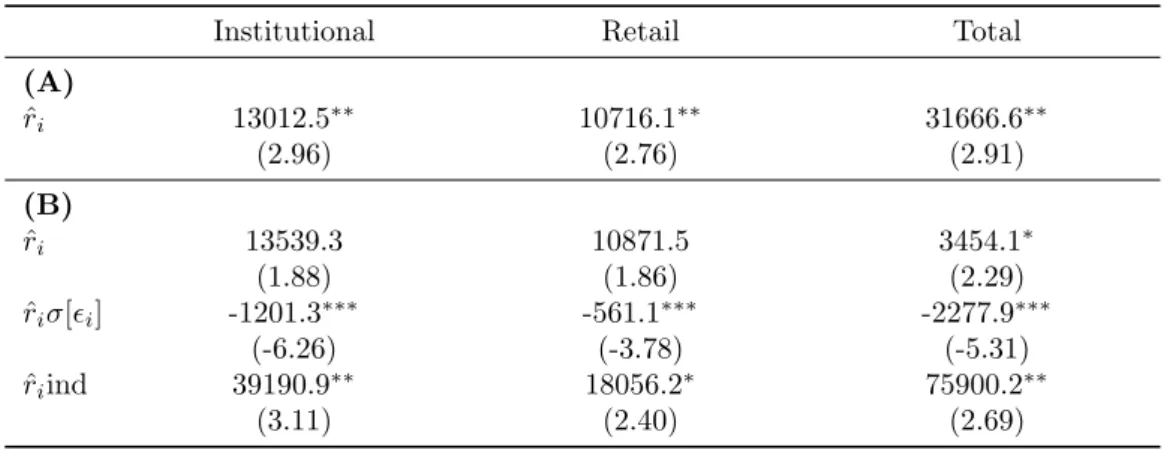
(A) ˆ ri 13012.5∗∗ 10716.1∗∗ 31666.6∗∗ (2.96) (2.76) (2.91) (B) ˆ ri 13539.3 10871.5 3454.1∗ (1.88) (1.86) (2.29) ˆ riσ[i] -1201.3∗∗∗ -561.1∗∗∗ -2277.9∗∗∗ (-6.26) (-3.78) (-5.31) ˆ riind 39190.9∗∗ 18056.2∗ 75900.2∗∗ (3.11) (2.40) (2.69) Equity Outflow

Institutional Retail Total

(A) ˆ ri -3880.2 -251.4 -2032.6 (-0.67) (-0.06) (-0.25) (B) ˆ ri -2563.5 4430.8 18541.6 (-0.16) (0.53) (1.04) ˆ riσ[i] -86.17 -478.9∗∗ -1208.4 (-0.16) (-2.98) (-1.88) ˆ riind 429.6 7037.2 1118.5 (0.05) (0.80) (0.05)

Equity Net flow

Institutional Retail Total

(A) ˆ ri 16892.7∗ 10967.5∗∗ 33699.2∗∗ (2.41) (2.56) (2.76) (B) ˆ ri 16102.6 6440.7 11912.5 (0.94) (0.75) (0.71) ˆ riσ[i] -1115.1∗ -82.15 -1069.5∗ (-2.03) (-0.48) (1.14) ˆ riind 38761.3∗∗∗ 11019.0 74781.7∗∗∗ (3.36) (1.35) (1.72)

Table 8: Coefficients of return variables in the Fixed Effects regression. These tables

are reported only for one measure of flow, raw flowF, and one measure of excess return,

αcapm. Control variables and time dummies are suppressed. The full regression results

(47)

5.2.1 Individual equity flows

Firstly, we find thatequity fund inflows are positively related to past relative returns.

This can be seen from model A on the left, and this result is clearly consistent independent of the flow and excess return measure used. This can be verified by looking at the full results in the appendix.

In general, we find that equity fund inflows are more easily explained by past

relative performance than outflows. One hypothesis is that if you have money to invest, it is logical to assume a rational evaluation of where to put them. Past re-turns are simple and intuitive measures to distinguish between options. However, withdrawal of money may be caused by reasons not directly related to fund perfor-mance. If you need the money, for whatever reason, you take them out. However, when investing money you may evaluate different investment options carefully.

Another interesting finding concerns the idiosyncratic risk of the equity funds

included in regression B. We find that past relative performance is less important

for flows to volatile equity funds. This can be seen from the negative coefficients in the table to the left which reduce the total effect of excess returns. Intuitively, this might be because past returns are less likely to be reproduced. There is less reason to assume performance persistence among these funds as they are relatively volatile. Consequently past returns do not seem like a relevant indication of fu-ture performance anymore. This tendency is confirmed in the appendix for equity inflows for all investors, but is also present for equity outflows for retail investors. Indeed, Huang et al. (2011) find evidence in support of our results. They show that the flow-performance sensitivity is weaker for funds with high idiosyncratic risk. Moreover, this dampening effect is stronger for more sophisticated investors.

In fact, we also document this. The negative coefficients found in relation to

idiosyncratic risk and equity fund inflows are consistently larger for institutional

investors than retail investors. This might indicate that institutional investors

account for fund-specific risk to a larger degree than retail investors when buying equity funds as this tendency is also present for some of the relative flow measures.

Furthermore, equity fund inflows are found to be much more sensitive to past

relative performance in bull markets, as seen from regression B. A possible hypoth-esis for this is closely related to our findings above. That is, in a declining market past returns may be of less importance as volatility and uncertainty thrive - the past is less likely to be descriptive of the future. In a rising, stable (bull) market the economic situation is arguably more predictable. Consequently, investors might turn to past performance to compare investment opportunities. This result is also clear in the complete results in the appendix.

Kim (2010) finds that when markets are highly volatile, which is generally the case in bear markets, relative returns are less relevant for flows. This is in agreement with our findings. Li et al. (2013) find that past performance is positively related to net equity fund flows, but, more interestingly, they find that this effect is stronger during bull markets than bear markets. This is also in accordance with our results. Also, as for the idiosyncratic volatility effect, it seems like this bull market effect is especially strong for institutional investors. The overall effect of simple excess returns on inflows is quite similar for retail and institutional investors, as

(48)

seen from model A, but the coefficients found for idiosyncratic volatility and the market indicator in model B are much larger in absolute value for institutional investors than retail investors. However, this finding is not obvious for all flow and excess return measures in the full results.

(49)

6 CONCLUSION

6 Conclusion

The purpose of this paper is to describe capital flows to and from Norwegian mutual funds. In the introduction the following question was posed: What are the determinants of capital flows in the Norwegian fund industry? The main findings of our research are given below.

Our first finding is thatinstitutional investors are likely to use a wider set of

market variables to evaluate investment opportunities. Retail investors are more

likely to concentrate on past returns within the relevant fund category. This finding

is supported by several studies. Clifford et al. (2011) find that retail investors are more sensitive to past performance than institutional investors. Huang et al. (2011) further find that institutional investors look beyond past returns to a greater degree than retail investors.

Another finding is that retail investors in equity funds are more likely to sell

their shares when equity funds as a category have performed well. They might be

eager to capitalize on previous gains. At the same time, bothretail and institutional

investors target specific equity funds that have outperformed competitors in the past

when buying funds. Indeed, Ivkovi´c and Weisbenner (2009) find that while outflows

are driven by absolute performance, inflows are driven by relative performance. This is in line with the results above where equity fund outflows are driven by market performance, whereas equity fund inflows are explained by the relative performance of specific funds.

Having established thatindividual equity fund inflows are sensitive to past

rel-ative returns, we further find that this relationship is stronger in bull markets.

Intuitively, past returns and the idea of performance persistence make more sense in a stable, non-volatile environment. Indeed, both Kim (2010) and Li et al. (2013) support our findings. Specifically, the latter paper finds that past performance is positively related to net equity fund flows, and that this effect is stronger in bull markets than bear markets.

Furthermore, we find thatflows to volatile equity funds are less affected by past

returns. Huang et al. (2011) support this result. Moreover, they find this effect to be larger for institutional investors which our results also indicate for inflows to equity funds. Once again, being able to reproduce past performance may be less likely for more volatile funds, explaining the reduced focus on past returns.

Additionally, we find indications thatbond and money market funds compete for

the same capital. Indeed, Ederington and Golubeva (2011) document reallocations

between these two fund categories depending on past returns. As they are relatively

similar in nature, this result seems quite intuitive. Also, we find that an increase

in stock market volatility drives retail investors out of money market funds. As a final comment, bond and money market flows are not investigated individ-ually, but only aggregated for each category because of data limitations. However, it would be highly interesting to analyze these flows on an individual fund level as we have done for equity funds.

(50)