Summary We used a physically based ecohydrological model to predict the water balance and growth responses of a mountain ash (Eucalyptus regnans F. Muell.) forest catchment to clear-felling and regeneration. The model, Topog-IRM, was applied to a 0.53 km2 catchment for a 3-year pretreatment period, and a 20-year period following clear-felling and re-seeding of 78% of the catchment area. Simulations were evalu-ated by comparing observed and predicted streamflows, rainfall interception and soil water values. The model faithfully simulated observed temporal patterns of overstory live stem carbon gain and produced a leaf area trajectory consistent with field observations. Cumulative throughfall was predicted within 1% of observations over an 18-year period. Over a 4-year period, predicted soil water storage in the upper 1.5 m of soil agreed well with field observations. There was fair correspondence between observed and predicted daily stream-flows, and the model explained 76% of the variation in monthly flows. Over the 23-year simulation period, the model overpre-dicted cumulative streamflow by 6%. We argue that there is a useful role for physically based ecohydrological models in the management of mountain ash forest catchments that cannot be satisfied by simple empirical approaches.
Keywords: ecohydrology, forest growth, modeling, water yield.
Introduction
Water for the city of Melbourne is harvested from 1550 km2 of forested catchments in the Central Highlands of Victoria, Aus-tralia. Ash forests, principally mountain ash (Eucalyptus reg-nans F. Muell.), cover just under half this area, but yield 80% of the streamflow because they grow on the higher rainfall sites.
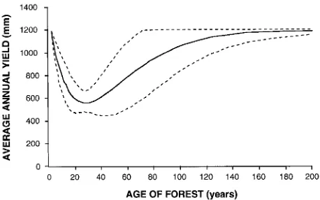
Regrowth mountain ash forests yield significantly less water than old growth stands because of differences in forest density and structure (Langford 1976, Jayasuriya et al. 1993). Kuczera (1985) developed an idealized curve describing the relation-ship between mean annual streamflow and mountain ash forest age (Figure 1). The curve is based on the measured hydrologic
responses of eight large catchments to a fire in 1939 and is constructed for the hypothetical case of a pure mountain ash forest catchment. It assumes that old growth forests yield an average runoff of 1195 mm year−1. It indicates that after disturbance caused by fire or logging and subsequent re-growth, runoff falls to 580 mm year−1 until age 27 years, after which yield slowly recovers over a period of around 150 years. However, the curve has wide error bands associated with it, particularly for forests aged 50 to 120 years, making it difficult to predict accurately when water yields will recover after disturbance. Moreover, because the curve is highly general-ized, variation that exists among mountain ash forest catch-ments with different site characteristics is masked. Despite these limitations, the curve has been used to predict water yield from eucalypt forest in morphoclimatic settings entirely differ-ent from the Cdiffer-entral Highlands (Moran 1988, Wilby and Gell 1994).
Vertessy et al. (1993) demonstrated that water yield from an old growth mountain ash stand could be predicted using a topographically based catchment model. That study assumed that the vegetation was in steady state and no attempt was made to simulate how the carbon and water balances change after a
Long-term growth and water balance predictions for a mountain ash
(
Eucalyptus regnans
) forest catchment subject to clear-felling and
regeneration
R. A. VERTESSY,
1,3T. J. HATTON,
1R. G. BENYON
2,3and W. R. DAWES
1 1 CSIRO Division of Water Resources, GPO Box 1666, Canberra, ACT 2601, Australia2 Melbourne Water, Box 4342, Melbourne, Victoria 3001, Australia
3 Cooperative Research Center for Catchment Hydrology, Monash University, Clayton, Victoria, Australia
Received March 2, 1995
Figure 1. Empirical relationship between mountain ash forest age and average annual water yield, after Kuczera (1985). Dashed lines indi-cate 95% confidence limits.
forest is perturbed. Here we report an application of a variant of this model, Topog-IRM, to a mountain ash forest catchment where vegetation changed abruptly from old growth to re-growth. The Topog-IRM model simulates the spatial and tem-poral changes in the forest carbon balance and the effect that this has on the catchment water balance.
Materials and methods Site description
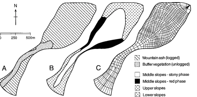
We applied Topog-IRM to the 0.53 km2 Picaninny catchment, which forms part of the Coranderrk experimental area estab-lished by the former Melbourne and Metropolitan Board of Works (now Melbourne Water Corporation) in 1955 (Howard and O’Shaughnessy 1971, Langford and O’Shaughnessy 1980a). Picaninny was originally covered by old growth mountain ash forest (about 200 years old), but between No-vember 1971 and March 1972, 78% of the catchment was clear-felled and re-seeded with mountain ash. Germination of the seed started in July 1972. Buffer vegetation (accounting for the remaining 22% of the catchment area) was retained around the stream course (Figure 2A). The adjacent 0.62 km2 Slip Creek catchment served as an untreated control catchment for Picaninny.
Picaninny has a mean slope of 37%, is south facing and has an elevation range of 230 to 780 m above mean sea level. Mean annual rainfall is 1180 mm (low for mountain ash forest) and is evenly distributed throughout the year with a mild spring maximum. Mean annual runoffs from the Picaninny and Slip Creek catchments for the 3 years before forest clearance were 332 and 406 mm, respectively. Hence, these catchments yield about one third of the annual streamflow assumed in the Kuczera (1985) model.
Vegetation consists mainly of mature (and eventually re-growth) mountain ash forest with a mixed hardwood under-story of mountain hickory wattle (Acacia frigrescens J.H. Willis), blanket leaf (Bedfordia arborescens Hochr.) and musk (Olearia argophylla Labill. (Benth.)). In the buffer area around the stream, mature mountain ash vegetation is mixed with hazel (Pomaderris aspera DC.), myrtle beech (Nothofagus cunninghamii (Hook.f.) Ørst.) and sassafras (Atherosperma
moschatum Labill.). The Coranderrk soils have been described in detail by Langford and O’Shaughnessy (1980b) who dis-criminate between upper, middle and lower slope soils (Fig-ure 2B). All soil groups are high in clay content (up to 70%) but are well structured and therefore fairly transmissive. Po-rosities range from 30 to 70%, and depth to bedrock varies between 5 and 20 m.
Hydrologic monitoring
Streamflow has been continuously monitored at Picaninny and Slip Creek since 1958. Rainfall and temperature have been continuously recorded at the Lower Coranderrk meteorologi-cal station (Figure 3) since late 1968. Between 1975 and 1983, soil water measurements were made at approximately monthly intervals at 12 sites within Picaninny (Figure 3). At each site, soil water measurements were made at 30-cm depth intervals with a neutron moisture meter to depths of between 1.5 and 5.1 m depending on local soil state. At two sites, throughfall measurements (rainfall less interception and stemflow) were made every 2 weeks beginning in October 1974 (Figure 3).
Forest growth monitoring
Starting in 1980, growth of the regenerating mountain ash vegetation was periodically monitored in 45 randomly located, permanent sample plots, each 100 or 200 m2 in area (Figure 3). Estimates of gross stem bole volumes, based on measurements of tree heights and stem diameters at 1.3 m above ground level, were recorded on eight occasions between December 1981 and January 1992. For each survey, total stem carbon (Cst) of the overstory was computed by:
Cst = Vbt Fw Dw Fc, (1) where Cst is total stem carbon in kg m−2, Vbt is gross bole volume in l m−2, Fw is the wood density fraction, assumed to be 0.32 (Dunn and Connor 1991), Dw is the density of cellu-lose, assumed to be 1.53 kg l−1, and Fc is the carbon fraction by weight of oven-dry wood, assumed to be 0.5.
Live stem carbon was computed as:
Csl = Vbs Fw Dw Fc, (2)
where Csl is live stem carbon in kg m−2, and Vbs is stem sapwood volume in l m−2. Bark and sapwood thicknesses used to calculate stem sapwood volume were based on an analysis of 263 mountain ash trees, selected randomly in stands of age 7, 20, 53 and 92 years.
Model description
Overview
Topog-IRM is a physically based ecohydrological model de-signed to predict the three dimensional water and plant carbon balances of heterogeneous catchments (Hatton et al. 1992, Dawes and Hatton 1993, Dawes et al. 1995). It links soil water processes, canopy microclimate, plant growth and catchment topography, and is composed of modules that solve energy and water balance and calculate plant growth. The model is driven by time-series inputs of daily rainfall, total daily solar radia-tion, mean daily temperature and humidity. It predicts daily rainfall interception, vertical and horizontal soil water distri-bution, the horizontal distribution of daily evapotranspiration from both the overstory and understory vegetation, daily evaporation from the soil--litter layer, and daily streamflow. The model also predicts daily changes in leaf, stem and root carbon of both the understory and overstory, and leaf fall and decomposition. The component algorithms used in the model are briefly described below.
The computational network
Topog-IRM uses a flow net defined by elevation contours and lines of steepest slope (O’Loughlin 1986, Dawes and Short 1994) (Figure 2C). An automated terrain analysis system has been designed to build the flow net and, for each element, to calculate terrain attributes (such as slope and aspect) that impact on the catchment water and carbon balance. Routines have also been developed to ascribe spatially variable catch-ment properties (such as soil or vegetation type) to specific elements.
Soil water dynamics
The soil water dynamics module in Topog-IRM is identical to that in the Topog-Yield model (Vertessy et al. 1993). Vertical soil water fluxes (unsaturated and saturated flows) are modeled in each element by a fast implicit solution of the Richards equation. In the lateral dimension, subsurface and overland flows run downslope within the flow net. Darcy’s law is used to model saturated subsurface flow, but no allowance is made for unsaturated lateral flow.
Evapotranspiration
Evaporation from the overstory, understory and soil layers is modeled on a daily time-step. For each layer, the surface radiation balance consists of four components: incoming shortwave radiation (a model input), reflected shortwave radia-tion from the surface, incoming longwave radiaradia-tion from the atmosphere, and emitted longwave radiation from the surface. Ignoring advection, for each catchment element, the radiation balance can be written as:
Rn = Rsd −Rsu + Rld −Rlu, (3)
where Rn is the net radiation, Rsd is the shortwave downward radiation, Rsu is the shortwave upward radiation, Rld is the longwave downward radiation, and Rlu is the longwave upward radiation. The shortwave downward radiation on a horizontal surface is modified according to the slope and aspect of the element (Klein 1977).
An approach similar to that of Monteith and Unsworth (1990) was adopted for modeling the radiation balance of each layer. By assuming all leaves are randomly distributed with horizontal inclination, the radiation balance for the overstory is written as follows:
Rsv1↓ = Rsd [1 − exp(−KeLAI1)] (4) Rsv1↑ = Rsd α1[1 − exp(−KeLAI1)] (5) Rlv1↓ = Rld [1 − exp(−KeLAI1)] (6) Rlv1↑ = Rlu [1 − exp(−KeLAI1)], (7) where the subscripts sv1 and lv1 indicate shortwave and long-wave radiation, respectively, for vegetation layer 1 (overstory), the arrows indicate the flux directions, Ke is the radiation extinction coefficient for the overstory, LAI1 is the cumulative leaf area index of the overstory, and α1 is the albedo of the overstory. Following Brutsaert (1982), the longwave radiation is estimated as:
Rld = εaσTa4 (8)
Rlu = εsσTa4 (9)
with
εa = 1.24(ea/Ta)1/7, (10)
where εa is the atmospheric emissivity, Ta is the air temperature in K, ea is the vapor pressure in kPa, εs is the surface emissivity (assumed to be 0.97), and σ is the Stefan-Boltzman constant.
The radiation balances of the understory canopy and the soil surface are treated in a similar fashion. The energy balance for the canopy and soil layers is thus:
Rnv1 = Rsv1↓−Rsv1↑ + Rlv1↓−Rlv1↑ (11) Rnv2 = Rsv2↓−Rsv2↑ + Rlv2↓−Rlv2↑ (12) Rng = Rsg↓−Rsg↑ + Rlg↓−Rlg↑, (13) where Rnv1, Rnv2 and Rng are the net radiation for overstory, understory and ground surface, respectively.
Evaporation (E) from the overstory, understory and soil surface is calculated by the Penman-Monteith equation:
E=sRn+ρcpDa/ra s+γ(1+rs/ra)
, (14)
where s is the slope of the saturation vapor pressure curve, Rn is net radiation, r is the air density, cp is the specific heat of air, Da is the vapor pressure deficit of the air, γis the psychometric constant, ra is the aerodynamic resistance, assumed to be constant (cf. Running and Coughlan 1988, Leuning et al. 1991, Hatton et al. 1992), and rs is the surface resistance. On a daily time-step, soil heat flux was assumed to be negligible.
For vegetation transpiration, the canopy conductance is cal-culated by the empirical model of Ball et al. (1987) as modified by Leuning (1995):
where g0 is a residual stomatal conductance, g1 is an empirical coefficient, A is assimilation rate, cs is the CO2 mol fraction at the leaf surface, Γ is the CO2 compensation point, Dc is the imposed vapor pressure deficit at the canopy surface, and Dc0 is an empirical coefficient.
In solving Equation 14 for the overstory, understory and soil layers, different values of Da are assumed for each layer. The vapor pressure deficit at the overstory canopy (Dc) is modified to reflect the effective deficit at the understory canopy surface (sensu Grantz and Meinzer 1990); this modified deficit (Dmod ) is calculated using the omega coefficient proposed by Jarvis and McNaughton (1986):
where Ωc is the decoupling coefficient, Deq is the equilibrium saturation deficit, and ε is s/γ. A similar approach is used to reduce the vapor pressure deficit below the understory for the soil surface, except instead of using Dc in Equation 16, the understory canopy value of Dmod is used.
Soil evaporation is calculated by the Penman-Monteith equation with the surface resistance set to zero if the soil surface is not air-dry, or determined by the method of Choud-hury and Monteith (1988) when in second phase drying:
rs = τl/pDm, (19)
where p is the porosity of the soil, Dm is the molecular diffusion coefficient for water vapor, τ is a tortuosity factor, and l is the depth of the air-dry soil layer as determined dynamically by the Richards equation solution of water content.
Plant growth
The plant growth model in Topog-IRM has been described in detail (Hatton et al. 1992, Dawes and Hatton 1993, Wu et al. 1994). The model assumes that the actual CO2 assimilation rate is dependent on a maximum rate and the relative availabilities of light, water and nutrients. It computes the assimilation index (r) of Wu et al. (1994): relative resource availabilities for water, nutrition and light, respectively, and mL is the modifier of light availability due to temperature. The mL modifier is based on a Gaussian distribu-tion of temperature effects parameterized by the optimal tem-perature and the temtem-perature at the half-saturation response. Finally, carbon assimilation (A) is calculated as:
A = rAmax , (21)
where Amax is the maximum mean daily assimilation rate of CO2.
Five carbon pools are defined: litter, leaf, root, live stem, and a soluble pool expressed as a fraction of leaf carbon. Mainte-nance respiration is calculated as a function of temperature (cf. Running and Coughlan 1988), and net photosynthesis is calcu-lated as assimilation less total respiration. When daily respira-tion exceeds assimilarespira-tion, carbon is taken from the soluble pool (if present), then from the leaf and root pools. Growth respiration is assumed to be a constant fraction of allocated carbon (Rauscher et al. 1990).
minimum mechanical and hydraulic support. Carbon alloca-tion to leaves, roots and stems is dynamic and follows the approach of Running and Gower (1991) in that the leaf/root ratio is based on the relative availabilities of above- and below-ground resources (sensu Chapin et al. 1987, Wilson 1988), in this case as calculated by the equation for r.
Increments to root carbon are distributed by dynamic allo-cation of carbon through the root zone. We assume that root carbon is continuous from the surface downward, that roots are added to the wettest (most favorable) region of soil, and that roots grow downward in search of water. The favorability of a soil region is a function of the availability of water.
Irrespective of daily assimilation, each of the three living carbon pools suffer daily decrements, representing the turn-over of leaves, bark and roots. Shedding from the two above-ground carbon pools, as well as any carbon from net negative assimilation, contributes to the litter pool. The litter pool de-cays as a function of temperature and water availability (Hat-ton et al. 1992).
Model application
Topog-IRM was applied to the Picaninny catchment for two phases, the pretreatment phase (January 1, 1969, to July 22, 1972) and the recovery phase (July 23, 1972, to July 18, 1992); however, the growth modeling capabilities of the model were only employed in the recovery phase. In the pretreatment phase, the leaf area index (LAI) of the forest was fixed at 2.0 for both the overstory and the understory.
A flow net comprised of 690 elements was computed (Fig-ure 2C). Elements varied in area between 188 and 3600 m2 with a mean of 885 m2. Soils and vegetation maps were overlain on the element network so that spatial variability of these properties was represented (Figures 2B and 2C).
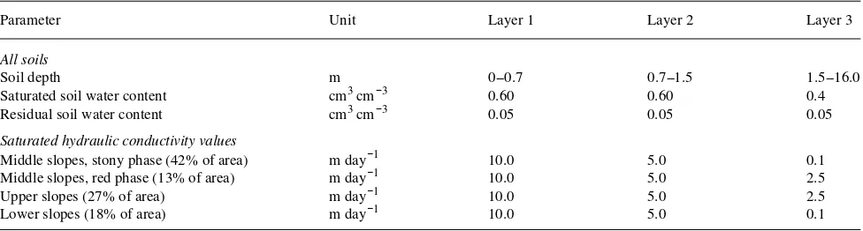
Four soil complexes were represented in the simulations (Figure 2B) (see Langford and O’Shaughnessy 1980b). In each complex, three separate soil layers were defined, spanning the depths 0--0.7, 0.7--2.0 and 2.0--16.0 m. The soil hydraulic properties ascribed to these layers in each complex are given in Table 1.
The forest was represented as a three-layer system, com-prised of overstory and understory vegetation and a litter layer.
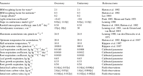
Eighteen parameters were used to define the physiological and energy balance properties of the vegetation (Table 2). Vegeta-tion parameter values used in the simulaVegeta-tion were based on a combination of published and measured values, although a few parameters (such as the respiration coefficients) were treated as calibration parameters. We assumed that nutrients were optimal (cf. Weston 1990).
The value used for the slope of the relationship between stomatal conductance and regrowth vegetation is similar to that reported by Leuning (1990) for Eucalyptus grandis W. Hill ex Maiden. Connor et al. (1977) reported a decrease in stomatal conductance in mature forest relative to regrowth forest of about 20% (derived from results in their Table 3). Given this observation and the fact that the stomatal conduc-tance algorithm used in Topog-IRM is linear with respect to the slope parameter (g1), the slope parameter was reduced by 20% for the pretreatment forest.
To evaluate the potential of the model to predict the conse-quences of forest disturbance on streamflow in ungauged catchments, simulations identical to those described above were performed on Picaninny but with modifications to catch-ment aspect and climate. In the first of these simulations, the catchment element network was rotated 180° to change the aspect from southerly to northerly. In the second of these simulations, the Picaninny catchment was modeled using a climate representative of a higher elevation site. The modified climate series was generated with MTCLIM (Running et al. 1987), a model that extrapolates meteorological data in moun-tainous terrain on the basis of lapse rates and an imposed rainfall and elevation gradient. Annual rainfall was approxi-mately double that measured at the Picaninny catchment to represent known changes at sites 1000 m higher in elevation. The resulting climate had a mean annual air temperature 2.9 °C lower, a mean annual vapor pressure deficit 0.18 kPa lower, and a mean daily solar radiation 0.5 MJ m−2 lower than the Lower Coranderrk meteorological station.
Results
Most results are plotted on a time axis that uses the time of forest clearance (July 1972) as an origin. Thus reference to Year 15 means 15 years after forest clearance.
Table 1. Soil parameters used in the Topog-IRM simulations for the Picaninny catchment. Four soils, each with three layers, were distributed across the catchment as shown in Figure 2C.
Parameter Unit Layer 1 Layer 2 Layer 3
All soils
Soil depth m 0--0.7 0.7--1.5 1.5--16.0
Saturated soil water content cm3 cm−3 0.60 0.60 0.4
Residual soil water content cm3 cm−3 0.05 0.05 0.05
Saturated hydraulic conductivity values
Middle slopes, stony phase (42% of area) m day−1 10.0 5.0 0.1
Middle slopes, red phase (13% of area) m day−1 10.0 5.0 2.5
Upper slopes (27% of area) m day−1 10.0 5.0 2.5
Forest growth
Eight observations of live stem carbon content were made between Years 9 and 20. Figure 4 compares observed mean overstory stem carbon with model predictions for two loca-tions in the catchment possessing extremes in radiation load-ing. The model slightly overestimated stem growth between Years 9 and 12, but at Year 20, the observed catchment mean stem carbon value of 2.4 kg m−2 was within the spatial range of predicted values. The observed trend of overstory stem
carbon was generally steeper than the model predictions, but stem carbon increments decreased after Year 15. The under-story stem carbon reached a peak of 0.42 kg m−2 at Year 9, and then declined slightly to 0.39 kg m−2 at Year 20. At the end of the simulation, overstory root carbon was 1.05 kg m−2.
Simulated mean catchment LAI for the mountain ash re-growth following logging increased monotonically to about 4.0 at Year 20 (Figure 5); however, because of spatial differ-ences in radiation across the catchment, LAI at particular
Table 2. Overstory and understory vegetation parameters used in the Topog-IRM simulations for the Picaninny catchment. Parameters used in the calibration of the growth model are indicated. Symbols: [o] = old growth forest, [r] = regrowth forest, and an asterisk denotes a dimensionless variable.
Parameter Overstory Understory Reference/note
IRM weighting factor for water* 2.1 2.1 Hatton et al. 1992
IRM weighting factor for nutrients* 0.3 0.3 Hatton et al. 1992
Canopy albedo* 0.2 0.2 Lee 1980
Light extinction coefficient* −0.42 −0.6 Pook 1985, Monsi and Saeki 1953
Slope in conductance model (g1)* 8.0[o], 11.0[r] 8.0[o], 11.0[r] Leuning 1990
Rainfall interception coefficient, mm LAI−1 day−1 0.30 0.30 Dunin et al. 1988, Hatton et al. 1992
Aerodynamic resistance, s m−1 15[o], 20[r] 30 Leuning et al. 1991, van de Griend and
van Boxel 1989
Maximum assimilation rate, µmols m−2 s−1 24.0 24.0 Leuning 1990, van den Driessche et al. 1971
Optimum temperature for assimilation, °C 20.0 20.0 Hatton et al. 1992, Küppers et al. 1987
Half saturation temperature, °C 10.0 10.0 Küppers et al. 1987
Light saturation value, µmols m−2 s−1 1000.0 800.0 Küppers et al.1987
Leaf respiration coefficient, kg kg−1°C−1 day−1 0.0140 0.0008 Calibrated parameter Stem respiration coefficient, kg kg−1°C−1 day−1 0.0010 0.0012 Calibrated parameter Root respiration coefficient, kg kg−1°C−1 day−1 0.0010 0.0010 Calibrated parameter
Leaf growth respiration, kg kg−1 0.65 0.65 Calibrated parameter
Stem growth respiration, kg kg−1 0.35 0.35 Calibrated parameter
Root growth respiration, kg kg−1 0.50 0.50 Calibrated parameter
Initial leaf carbon value, kg m−2 0.16[o], 0.03[r] 0.16[o], 0.006[r] Field observations Initial stem carbon value, kg m−2 2.6[o], 0.03[r] 1.6[o], 0.006[r] Field observations Initial root carbon value, kg m−2 0.164[o], 0.012[r] 0.102[o], 0.002[r] Field observations
Figure 4. Observed and predicted live stem carbon values for the mountain ash overstory in the Picaninny catchment for 1969--1991. The range in predicted values over the catchment is indicated, along with the mean of observed values. Spatial variation in stem carbon was due to the pattern of solar radiation across the catchment.
locations varied between 3.1 and 4.7. Understory LAI in-creased to a maximum of 0.9 at Year 10, and then declined slowly to 0.8 by Year 20.
The availability of soil water was near its maximum value throughout the simulation period. With nutrition assumed to be optimal, the IRM scalar for assimilation of CO2 covaried almost solely with the temporal pattern of solar radiation; temperature effects on photosynthesis were minimal.
Throughfall and evapotranspiration
Throughfall measurements commenced 2.5 years after forest clearance and totaled 176.55 cm by Year 20 (86.5% of gross rainfall). The model estimate of throughfall for the same period was 178.15 cm. Figure 6 compares cumulative observed and predicted throughfall. The two curves diverge slightly at the beginning, but by Year 20 there is only a 1% difference be-tween the cumulative totals.
Simulated evaporation (spatially averaged over the catch-ment) from the overstory, understory and soil appear in Fig-ure 7 as annual totals. There was little variation in annual evaporation rates before forest clearance, despite variation in
rainfall over this period. In the first few years following log-ging, there was an immediate increase in soil evaporation, and transpiration was mostly limited to the unlogged buffer vege-tation. Regrowth of the mountain ash led to increases in tran-spiration over the rest of the simulation and exceeded pretreatment rates after only 5 years. Transpiration from the understory recovered more slowly and approximated soil evaporation after 7 years of regrowth. Simulated soil water potentials did not significantly limit transpiration in any year. Before logging, maximum summer daily evaporation rates for the overstory, understory and soil were 2.0, 1.1 and 0.4 mm day−1 , respectively, and the corresponding values at Year 20 were 4.1, 0.5 and 0.5 mm day−1. In midwinter, typical daily evaporation rates for the overstory, understory and soil were 0.14, 0.07 and 0.06 mm day−1, respectively, before logging, and the corresponding values at Year 20 were 0.2, 0.02 and 0.05 mm day−1.
Soil water
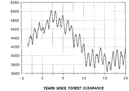
Mean winter time soil water storage within the catchment rose from about 4500 mm in the pretreatment period to 5000 mm about 2.5 years after forest clearance (Figure 8). Soil water storage returned to pretreatment values around Year 6, then declined to a stable value of about 4100 mm in Year 11. Despite falling water levels, the seasonal amplitude of soil water change tended to increase as regrowth vegetation became established. Mean summer soil water depletion increased from 14 mm m−1 in the pretreatment phase to 23 mm m−1 between Years 10 and 20 (Figure 8).
There was good correspondence between observed and pre-dicted soil water storage in the upper 1.5 m of soil between Years 4.5 and 8.5 (January 1977 to January 1981) (Figure 9). The predicted curve shows mean daily soil water storage for all catchment elements outside the buffer region (Figure 2A). The observations are mean values from 12 bore holes scattered throughout the catchment (Figure 3). Both the seasonal ampli-tude and the timing of changes in soil water storage are well represented by the model, and predictions are within the ob-served 95% confidence limits.
Figure 6. Observed and predicted cumulative daily throughfall in the Picaninny catchment for 1974--1991. Observed throughfall includes estimated stemflow, taken as 4% of gross rainfall.
Figure 7. Simulated annual evaporation from overstory, understory and soil in the Picaninny catchment for 1969--1991. These estimates do not include interception losses. Arrow shows time of forest clear-ance.
Daily and monthly runoff
Model predictions of daily catchment runoff generally agreed with field observations (Figures 10A and 10B). Although the model tended to underpredict base flow rates and overpredict peak flows, these errors compensated one another and became insignificant when runoff was aggregated on a monthly basis as shown in Figure 11, which shows good agreement between observed and predicted monthly runoff (r2 = 0.76, n = 286).
Annual runoff
Although annual catchment rainfall fluctuated during the 23-year simulation, there was a clear temporal trend in annual catchment runoff with an initial increase after forest clearance, followed by a sustained decrease in runoff relative to pretreat-ment flows (Figure 12). Observed annual catchpretreat-ment runoff from Picaninny rose from around 300 mm in the pretreatment phase to 700 mm in Year 2 (1974) and then declined to about 200 mm in Year 7 (1979). This trend is reinforced when annual runoff from Picaninny is compared to annual runoff from the adjacent Slip Creek control catchment (Figure 13). In the
pretreatment phase, Picaninny yielded about 80% of the runoff volume of the wetter Slip Creek catchment; however, within 2 years of forest clearance, Picaninny yielded twice as much runoff as Slip Creek and then gradually returned to pretreat-ment flow levels by Year 6 after logging. From Year 6 onward,
Figure 9. Observed and predicted mean catchment soil water storage, 0--1.5 m depth, in the Picaninny catchment: (A) January 1977 to January 1979, and (B) January 1979 to January 1981. Dots are the observed values with 95% confidence intervals.
Figure 11. Observed versus predicted monthly runoff from the Pican-inny catchment for 1969--1991. The diagonal line indicates a 1/1 relationship.
Figure 10. Observed and predicted daily runoff in the Picaninny catchment: (A) 200-day sequence in the pretreatment phase, and (B) 200-day sequence in the regrowth phase.
Figure 12. Annual rainfall, and observed and predicted annual runoff for the Picaninny catchment for 1969--1991. Reduced discharge fol-lowing forest regrowth is largely independent of the rainfall pattern. Arrow shows time of forest clearance.
annual runoff from Picaninny declined below pretreatment ratios until 1983 when it stabilized at about 45% of the Slip Creek runoff.
Predicted annual runoff generally agreed with observed val-ues throughout the 23-year simulation (Figure 12), though there was a systematic overprediction in the years 1975 to 1983 (Years 3 to 11 after forest clearance). Total observed and predicted runoff values for the entire simulation period were 5947 and 6317 mm, amounting to a 6.2% overprediction in runoff.
Scenario modeling
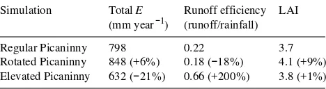
Table 3 shows the results from the two applications to two hypothetical catchments with varying aspect and elevation. Rotating the Picaninny catchment to a northerly aspect re-sulted in a 9% increase in LAI at Year 20, with a 6% increase in total annual evaporation (E), and thus reduced runoff effi-ciency. Application of a high elevation climate resulted in only a 1% increase in LAI, but a significant decrease (21%) in evaporation. This and the enhanced rainfall resulted in a treb-ling of runoff efficiency.
Discussion
Throughfall and evapotranspiration
There was close agreement between observed and predicted throughfall (Figure 6) despite the simplicity of the interception algorithm employed in Topog-IRM, which makes no allow-ance for differences in interception caused by variations in rainfall intensity. Although it is likely that discrete daily throughfall predictions would often be in error, it appears that these errors are compensatively smoothed over time. We note that the throughfall results are based on an a priori estimate for the leaf storage coefficient of 0.3 mm LAI−1 as reported for E. maculata Hook. forests by Dunin et al. (1988) and Hatton et al. (1992).
The seasonal range in simulated evaporation was greater than expected, with winter rates being low. By scaling leaf conductance measurements, Legge and Connor (1985) esti-mated peak summer evaporation rates from a mature mountain ash overstory to be 4.1 mm day−1, which is slightly more than the peak rates for total evapotranspiration in our pretreatment simulations. Based on sap flow measurements at a higher elevation site than Picaninny, Dunn and Connor (1993)
re-ported overstory summer transpiration for 50- and 230-year-old mountain ash stands of 2.04 and 0.77 mm day−1, respec-tively. Their annual estimates for 50- and 230-year-old stands were 679 and 296 mm, respectively. Given that the simulated LAI at Year 20 is apparently approaching a maximum, these values agree well with the model estimates at that age (669 mm) and for the old growth pretreatment condition (350 mm). Further, Dunn and Connor (1993) estimated understory contri-butions to total plant water use in the old growth forest to be 27%; in the pretreatment simulations, we predicted a value of 34%.
Simulated annual evaporation rates also agree with esti-mates by Langford et al. (1982) for the Picaninny catchment based on the difference between streamflow and estimated interception losses; these authors report pretreatment total evaporation losses of 620 mm in both 1969 and 1975 compared with values of 633 and 610 mm, respectively, in our simula-tions. Feller (1981) used soil water, rainfall and runoff data to estimate evaporative losses for the Year 1978, exclusive of interception, for a nearby, higher elevation mountain ash catch-ment receiving 1631 mm of rainfall and reported a value of 620 mm. The model estimate for Picaninny in 1978 was 710 mm, which is expected because there are more annual sunshine hours and warmer temperatures in this catchment.
Most of the annual variation in evaporation from canopies or soil was accounted for by changes in LAI, even in the presence of large variations in annual rainfall. Our soil water balance calculations indicate that soil matric potentials remain favorable for transpiration (and soil evaporation) throughout the year. We conclude that evaporation in mountain ash forests is almost entirely energy limited, with annual patterns of net radiation and temperature being conservative from year to year. This may simplify inferences about the effect of forest management on runoff (at least in this forest and edaphic environment), particularly when combined with observed (im-posed) estimates of LAI development. If LAI data can be made available from remote sensing technology (sensu Running et al. 1989), the need for a complex growth and evaporation model may be eliminated.
Forest growth
Apart from stem carbon measurements, there are few observa-tions with which to compare the simulated growth responses following logging in the Picaninny catchment. The simulated value of average catchment LAI for the mountain ash regrowth at Year 15 was 3.6, compared to a measured average value of 3.4 (range of 0.97 to 6.62) (Orr et al. 1986). Using an LAI-2000 leaf area meter (Li-Cor Inc., Lincoln, NE), O’Sullivan (pers. comm.) determined that total LAI was 4.7 at stand age 22 years at Picaninny; the sum of simulated overstory and understory LAI was 4.8 at age 20 years. The monotonicity of the LAI response in our simulations is somewhat at variance with observations for a regrowth plot at a nearby catchment with mountain ash in which LAI peaked at 5.1 at age 9 years (Vertessy et al. 1995) and declined to 4.4 at age 12 years (O’Sullivan, pers. comm.). Ashton (1976) argued that radiation interception increases in these forests to about age 40 years,
Table 3. Results of Topog-IRM simulations for the Picaninny catch-ment during the regrowth phase (1972--1991), indicating effects of changing aspect and elevation (climate). Bracketed numbers indicate percent change relative to baseline simulation. All LAI values shown are catchment averages.
Simulation Total E Runoff efficiency LAI
(mm year−1) (runoff/rainfall)
Regular Picaninny 798 0.22 3.7
though this includes understory effects. Our simulations indi-cated that LAI would continue to increase past age 20 years.
Feller (1980) estimated a root carbon equivalent of 3.1 kg m−2 in the top 100 cm of soil of a stand at age 40 years, which is almost three times the amount simulated at 20 years in this study, although Feller’s estimate included nonliving root ma-terial. Incoll (1979) found 99.7% of fine roots (< 5 mm in diameter) in the upper 105 cm of soil, but with some roots extending to 2.5 m. Ashton (1975) indicated that trees of age 23 years have rooting distributions to over 4 m, compared to simulated root carbon at age 20 years which grew to 5 m depth in this study. We conclude that although our simulated rooting distributions develop appropriately, the predicted root biomass may be underestimated.
Our simulations suggest that after 10 years of regrowth, understory begins to thin. Vertessy et al. (1995) estimated understory live stem carbon at stand age 15 years to be 0.97 kg m−2 which is twice the simulated value for Picaninny. How-ever, their estimate was for a stand where the overstory had been repeatedly subject to severe insect attack that aided un-derstory development.
There are strong dependencies of throughfall and evapora-tion on LAI within Topog-IRM. Although there is good overall agreement between observed and predicted throughfall, the cumulative estimates (Figure 6) depart in the early half of the simulation and are roughly parallel thereafter, indicating that the model did not develop the canopy quickly enough. Similar inferences may be drawn from the runoff results (Figure 12). Although the predicted annual runoff values for the pretreat-ment phase and the final 8 years of the simulation are good, there is a period between Years 6 and 11 that indicates too little evaporation from the system. Given the previous observation that too much stem carbon was accrued during this phase, this may indicate that the carbon allocation algorithm favored stem too much over leaves during this phase of the simulation.
Extrapolation of the overstory LAI results indicates a long-term maximum LAI at about 30--40 years after forest clear-ance, which is in broad agreement with observations by Ashton (1976). After this age, stand thinning and the apparent lack of gap-replacement recruitment of mountain ash leads to a long-term decline in overstory LAI and subsequent increase in understory LAI to roughly equivalent values (2.0). Topog-IRM is a ‘‘big leaf’’ model and hence does not represent trees as individuals, nor does it represent the stochastic processes lead-ing to forest thinnlead-ing. Consequently, the model would need to be modified to simulate forest growth beyond about 40 years in this forest type.
Although the agreement between observed and predicted live stem carbon was largely dependent on calibration of the respiration coefficients, it should be noted that Topog-IRM does not simulate leaf, root and stem growth independently. Thus the resulting balance among these components is neither predetermined nor subject to independent calibration. In this sense, the agreement with observations of these components is a reasonable test of the assimilation and allocation logic of the model, at least over the time scales involved in the reported simulations.
Soil water and runoff
The observed soil water data support our model predictions of soil water drainage and plant water uptake (Figure 9). The comparison is restricted to the upper 1.5 m of the soil profile because deeper readings were taken at only a few of the 12 bores in the catchment. We conclude that 12 bores was a marginal number for estimating mean water content across the catchment; however, the accuracy of the cumulative runoff predictions over the 23-year simulation period is probably within the accuracy of the measured climatic inputs and stream gauging.
The model simulated base flow behavior well but performed less well during and immediately after large storm events. The model had a tendency to overpredict peak flows (suggesting exaggeration of the contributing runoff area) and predicted flow recessions which were too steep (indicating exaggeration of the drainage rate) (Figure 10A). During heavy rain events, the model produced daily flow predictions that were worse than those shown in Figure 10A. It may be possible to rectify this problem with better parameterization of the catchment soils.
The model was able to simulate monthly and annual runoff from Picaninny during a period of variable land cover (Fig-ures 11 and 12), although there are some systematic errors, particularly in the annual flow predictions. One of the discrep-ancies between observed and predicted annual flows is the overprediction of runoff between 1978 and 1983 (Years 6--11). This result suggests that we underestimated LAI during this period, though this conflicts with our finding that throughfall was modeled accurately over this period. It is possible that stomatal conductances are higher than we assumed in the first few years of regrowth and begin to decline from age 11 years onward.
Scenario modeling
In catchments where land cover is static and streamflow is gauged, empirical relationships between rainfall and runoff are robust predictors of catchment runoff (e.g., Post et al. 1993). However, when land cover is dynamic, as in vigorously grow-ing forest, such relationships cannot be used to predict runoff because the water balance is determined by the course of leaf area development. Similarly, empirical runoff relationships are problematic to transfer to ungauged sites where catchment properties differ (Moran 1988). Physically based, distributed parameter models such as Topog-IRM provide a sounder basis for predicting the hydrologic impacts of forest disturbance in systems characterized by changing land cover and spatially variable catchment properties.
instance can be attributed to the use of inappropriate tempera-ture and humidity data and soil profiles associated with south-erly aspects. For instance, we know that soils at this elevation and aspect tend to be thinner or even skeletal; had we used these less favorable soils in this simulation, the forest canopy would not have performed so well. The high elevation scenario attempted to covary all climate parameters with elevation, but retained the same soil properties and topography. This resulted in elevated catchment runoff efficiencies of about 66% of rainfall, a value quite similar to the runoff for a real catchment (Myrtle II) in years with rainfall approaching this amount (Vertessy et al. 1993).
If models such as Topog-IRM are to be used in scenario modeling across and between regions, it is essential to repre-sent the spatial covariance of landscape properties accurately. For this reason, continuing effort is needed in the acquisition and handling of regional geographical data pertaining to topo-graphy, soils, land cover and climate. Further, the scenario modeling is only valid if the baseline calibration has resulted in a parameterization that minimizes compensating errors in processes (Sorooshian et al. 1983, Beven 1993).
We note that the calibration procedure adopted in these simulations was based on reproducing observed patterns of pretreatment runoff and stand development during the re-growth phase. The resulting predictions of evaporation, inter-ception and soil water distribution generally agreed well with observations based on a priori parameter values obtained from the literature and direct measurement. The finding that not only the resulting runoff estimations following logging were accu-rate but that the partitioning of the rest of the water balance was correct suggests that our model parameterization is sound and appropriate for extrapolation to other sites. Further, we note that the calibrated vegetation parameters related to respiration and allocation (Table 2) are in principle species specific (i.e., genetically determined) and thus transferable to other moun-tain ash sites.
Conclusions
After clear-felling in 1972, the Picaninny catchment under-went profound water balance changes that persisted for at least 20 years. Catchment runoff increased initially then decreased to well below pretreatment values as vigorous regrowth forest was established. This response is qualitatively consistent with the empirical model of Kuczera (1985), although the magni-tude and timing of the response differed because of the specific climatic conditions of the Picaninny site. The Kuczera model is based on a regionally averaged response to disturbance but is inadequate for planning at small catchment scales where site differences are important. We argue that to model this response over the range of environments in the Melbourne Water supply area, it is essential to model the forest recovery and its interac-tions with the water and energy balances given local site characteristics.
Model estimates of stem carbon and leaf area development during the regrowth phase in the Picaninny catchment agreed with field observations. This agreement, in combination with
accurate representation of the surface energy balance, rainfall interception and catchment drainage meant that we were able to simulate catchment runoff accurately. The strong depend-ence of mountain ash forest growth and evaporation on avail-able energy suggests a potential for simple representations of these processes and demonstrates the utility of physically based ecohydrological models in the development of practical management tools.
Acknowledgments
We thank Jamie Margules and Ian Watson for their help with data preparation. Melbourne Water Corporation kindly provided access to their extensive database for this project. Our thanks are extended to Craig Beverly, David Short, Lu Zhang, Tony Butt and Emmett O’Loughlin who have been active in the development of Topog. Kent Rich kindly assisted with the diagrams.
References
Ashton, D.H. 1975. The root and shoot development of Eucalyptus regnans F. Muell. Aust. J. Bot. 23:867--887.
Ashton, D.H. 1976. The development of even-aged stands of Eucalyp-tus regnans F. Muell. in central Victoria. Aust. J. Bot. 24:397--414. Ball, J.T., I.E. Woodrow and J.A. Berry. 1987. A model predicting stomatal conductance and its contribution to the control of photo-synthesis under different environmental conditions. In Progress in Photosynthesis Research. Vol. IV. Ed. J. Biggins. Martinus Nijhoff Publishers, The Netherlands, pp 221--224.
Beven, K. 1993. Prophecy, reality and uncertainty in distributed hydro-logical modelling. Adv. Water Resour. 16:41--51.
Brutsaert, W.H. 1982. Evaporation into the atmosphere. D. Reidel Publishing Company, Dordrecht, The Netherlands, 299 p. Chapin, F.S., III, A.J. Bloom, C.B. Field and R.H. Waring. 1987. Plant
response to multiple environmental factors. BioScience 37:49--57. Choudhury, B.J. and J.L. Monteith. 1988. A four-layer model for the
heat budget of homogeneous land surfaces. Q. J. R. Meteorol. Soc. 114:373--398.
Connor, D.J., N.J. Legge and N.C. Turner. 1977. Water relations of mountain ash (Eucalyptus regnans F. Muell.) forests. Aust. J. Plant Physiol. 4:753--762.
Dawes, W. and T.J. Hatton. 1993. Topog_IRM 1. Model description. CSIRO Division of Water Resources, Technical Memorandum 93/5, 33 p.
Dawes, W. and D.L. Short. 1994. The significance of topology for modeling the surface hydrology of fluvial landscapes. Water Re-sour. Res. 30:1045--1055.
Dawes, W.R., L. Zhang, T.J. Hatton, P.H. Reece, G. Beale and I. Packer. 1995. Application of a distributed parameter ecohydrologi-cal model (TOPOG_IRM) to a small cropping rotation catchment. J. Hydrol. In press.
Dunin, F.X., E.M. O’Loughlin and W. Reyenga. 1988. Interception loss from eucalypt forest: lysimeter determination of hourly rates for long term evaluation. Hydrol. Processes 2:315--329.
Dunn, G.M. and D.J. Connor. 1991. Transpiration and water yield in mountain ash forest. Land and Water Resources Research and Development Corporation, Project P88/37, 61 p.
Dunn, G.M. and D.J. Connor. 1993. An analysis of sap flow in mountain ash (Eucalyptus regnans) forests of different age. Tree Physiol. 13:321--336.
Feller, M.C. 1981. Water balances in Eucalyptus regans, E. obliqua
and Pinus radiata forests in Victoria. Aust. For. 44:153--161. Grantz, D.A. and F.C. Meinzer. 1990. Stomatal response to humidity
in a sugarcane field: simultaneous porometric and microme-teorological measurements. Plant Cell Environ. 13:27--37. Hatton, T.J., J. Walker, W. Dawes and F.X. Dunin. 1992. Simulations
of hydroecological responses to elevated CO2 at the catchment
scale. Aust. J. Bot. 40:679--696.
Howard, N.H. and P.J. O’Shaughnessy. 1971. First progress report, Coranderrk. Melbourne and Metropolitan Board of Works, Catch-ment Hydrology Research Report No. MMBW-W-0001, 177 p. Incoll, W.D. 1979. Root system investigations in stands of Eucalyptus
regnans F. Muell. Forests Commission Victoria Research Branch Report No. 136, 16 p.
Jarvis, P.G. and K.G. McNaughton. 1986. Stomatal control of transpi-ration: scaling up from a leaf to region. Adv. Ecol. Res. 15:1--49. Jayasuriya, M.D.A., G. Dunn, R. Benyon and P.J. O’Shaughnessy.
1993. Some factors affecting water yield from mountain ash ( Euca-lyptus regnans) dominated forests in south-east Australia. J. Hydrol. 150:345--367.
Klein, S.A. 1977. Calculation of monthly average insolation on tilted surfaces. Sol. Energy 19:325--329.
Kuczera, G.A. 1985. Prediction of water yield reductions following a bushfire in ash-mixed species eucalypt forest. Melbourne and Met-ropolitan Board of Works, Catchment Hydrology Research Report No. MMBW-W-0014, 163 p.
Küppers, M., A.G. Swan, D. Tompkins, W.C.L. Gabriel, B.I.L. Küp-pers and S. Linder. 1987. A field portable system for the measure-ment of gas exchange of leaves under natural and controlled conditions: examples with field-grown Eucalyptus pauciflora Sieb. ex Spreng. ssp. pauciflora, E. behriana F. Muell. and Pinus radiata
D. Don. Plant Cell Environ. 10:425--435.
Langford, K.J. 1976. Change in yield of water following a bushfire in a forest of Eucalyptus regnans. J. Hydrol. 29:87--114.
Langford, K.J., R.J. Moran and P.J. O’Shaughnessy. 1982. The Coran-derrk experiment----the effects of roading and timber harvesting in a mature mountain ash forest on streamflow yield and quality. In
Proceedings of the First National Symposium on Forest Hydrology, Melbourne, pp 92--102.
Langford, K.J. and P.J. O’Shaughnessy. 1980a. Second progress report, Coranderrk. Melbourne and Metropolitan Board of Works, Catch-ment Hydrology Research Report No. MMBW-W-0010, 394 p. Langford, K.J. and P.J. O’Shaughnessy. 1980b. A study of the
Coran-derrk soils. Melbourne and Metropolitan Board of Works, Catch-ment Hydrology Research Report No. MMBW-W-0006, 215 p. Lee, R. 1980. Forest hydrology. Columbia Univ. Press, New York, 349 p. Legge, N.J. and D.J. Connor. 1985. Relating water potential gradients in mountain ash (Eucalyptus regnans F. Muell.) to transpiration rate. Aust. J. Plant Physiol. 12:89--96.
Leuning, R. 1990. Modelling stomatal behaviour and photosynthesis of Eucalyptus grandis. Aust. J. Plant Physiol. 17:159--175. Leuning, R. 1995. A critical appraisal of a combined
stomatal-photo-synthesis model for C3 plants. Plant Cell Environ. 18:339--355.
Leuning, R., P.E. Kriedemann and R.E. McMutrie. 1991. Simulation of evapotranspiration by trees. Agric. Water Manage. 19:205--221. Monsi, M. and T. Saeki. 1953. Über den Lichtfaktor in den Pflan-zengezellschaften und seine Bedeutung für die Stoffproduktion. Jpn. J. Bot. 14:22--52.
Monteith, J.L. and M.H. Unsworth. 1990. Principles of environmental physics. 2nd Edn. Routledge, Chapman and Hall, New York, 291 p. Moran, R. 1988. The effects of timber harvesting operations on streamflows in the Otway Ranges. Department of Water Resources Victoria, Report No. 47, 172 p.
O’Loughlin, E.M. 1986. Prediction of surface saturation zones in natural catchments by topographic analysis. Water Resour. Res. 22:794--804.
Orr, S., D. Bennett, J. Snodgrass, J. Hoenen, G. Winter and C. Burley. 1986. A leaf area index for Eucalyptus regnans age 15 years. Coranderrk Leaf Area Project Report, Melbourne Metropolitan Board of Works, Melbourne, 16 p.
Pook, E.W. 1985. Canopy dynamics of Eucalyptus maculata Hook. III. Effects of drought. Aust. J. Bot. 33:65--79.
Post, D.A., A.J. Jakeman, I.G. Littlewood, P.G. Whitehead and M.D.A. Jayasuriya. 1993. Modelling land cover induced variations in hydrologic response: Picaninny Creek, Victoria. In Proceedings of the International Congress on Modelling Simulation. Eds. A. McAleer and A.J. Jakeman. Uniprint, Perth, pp 43--48.
Rauscher, H.M., J.G. Isebrands, G.E. Host, R.E. Dickson, D.I. Dick-mann, T.R. Crow and D.A. Michael. 1990. ECOPHYS: An eco-physiological growth process model for juvenile poplar. Tree Physiol. 7:255--281.
Running, S.W. and J.C. Coughlan. 1988. A general model of forest ecosystem processes for regional applications. I. Hydrologic bal-ance, canopy gas exchange and primary production processes. Ecol. Modell. 42:125--154.
Running, S.W. and S.T. Gower. 1991. FOREST-BGC, A general model of forest ecosystem processes for regional applications. II. Dynamic carbon allocation and nitrogen budgets. Tree Physiol. 9:147--160.
Running, S.W., R.R. Nemani and R.D. Hungerford. 1987. Extrapola-tion of synoptic meteorological data in mountainous terrain and its use for simulating forest evapotranspiration and photosynthesis. Can. J. For. Res. 17:472--483.
Running, S.W., R.R. Nemani, D.L. Peterson, L.E. Band, D.F. Potts, L.L. Pierce and M.A. Spanner. 1989. Mapping regional forest evapotranspiration and photosynthesis by coupling satellite data with ecosystem simulation. Ecology 70:1090--1101.
Sorooshian, S., V.K. Gupta and J.L. Fulton. 1983. Evaluation of maximum likelihood parameter estimation techniques for concep-tual rainfall--runoff models: influence of calibration data variability and length on model credibility. Water Resour. Res. 19:251--259. van den Driessche, R., D.J. Connor and B.R. Tunstall. 1971.
Photosyn-thetic response of brigalow to irradiance, temperature and water potential. Photosynthetica 5:210--217.
van de Griend, A.A. and J.H. van Boxel. 1989. Water and surface energy balance model with a multilayer canopy representation for remote sensing purposes. Water Resour. Res. 25:949--971. Vertessy, R.A., R.G. Benyon, S.K. O’Sullivan and P.R. Gribben. 1995.
Relationship between stem diameter, sapwood area, leaf area and transpiration in a young mountain ash forest. Tree Physiol. 15:559--567.
Vertessy, R.A., T.J. Hatton, P.J. O’Shaughnessy and M.D.A. Jayas-uriya. 1993. Predicting water yield from a mountain ash forest catchment using a terrain analysis based catchment model. J. Hy-drol. 150:665--700.
Weston, C.J. 1990. Recovery of nutrient cycling in Eucalyptus regnans
forests following disturbance. Ph.D. Thesis. University of Mel-bourne, MelMel-bourne, Australia, 133 p.
Wilby, R.L. and P.A. Gell. 1994. The impact of forest harvesting on water yield: modelling hydrological changes detected by pollen analysis. Hydrol. Sci. J. 39:471--486.
Wilson, J.B. 1988. A review of evidence on the control of shoot:root ratio in relation to models. Ann. Bot. 61:433--49.