Gauge Theories on Deformed Spaces
⋆Daniel N. BLASCHKE †, Erwin KRONBERGER ‡, Ren´e I.P. SEDMIK ‡ and Michael WOHLGENANNT ‡
† Faculty of Physics, University of Vienna, Boltzmanngasse 5 A-1090 Vienna, Austria
E-mail: [email protected]
‡ Institute for Theoretical Physics, Vienna University of Technology,
Wiedner Hauptstrasse 8-10, A-1040 Vienna, Austria
E-mail: [email protected], [email protected],
Received April 13, 2010, in final form July 14, 2010; Published online August 04, 2010 doi:10.3842/SIGMA.2010.062
Abstract. The aim of this review is to present an overview over available models and approaches to non-commutative gauge theory. Our main focus thereby is on gauge models formulated on flat Groenewold–Moyal spaces and renormalizability, but we will also review other deformations and try to point out common features. This review will by no means be complete and cover all approaches, it rather reflects a highly biased selection.
Key words: noncommutative geometry; noncommutative field theory; gauge field theories; renormalization
2010 Mathematics Subject Classification: 81T13; 81T15; 81T75
Contents
1 Introduction 2
2 Canonical deformation 8
2.1 Early approaches . . . 9
2.1.1 Scalar field theories . . . 10
2.1.2 Gauge field theories . . . 10
2.2 Θ-expanded theory . . . 11
2.2.1 Seiberg–Witten maps . . . 12
2.2.2 NC Standard Model . . . 14
2.3 The Slavnov approach . . . 17
2.3.1 The Slavnov-extended action and its symmetries . . . 18
2.3.2 Further generalization of the Slavnov trick. . . 22
2.4 Models with oscillator term . . . 23
2.4.1 The Grosse–Wulkenhaar model . . . 23
2.4.2 Extension to gauge theories . . . 24
2.4.3 Induced gauge theory . . . 30
2.4.4 Geometrical approach . . . 32
2.5 Benefiting from damping – the 1/p2 approach . . . 33
2.5.1 Gribov’s problem and Zwanziger’s solution . . . 34
2.5.2 The long way to consistent gauge models . . . 36
2.5.3 Localization . . . 38
⋆This paper is a contribution to the Special Issue “Noncommutative Spaces and Fields”. The full collection is
2.5.4 BRSW model . . . 42
2.6 Time-ordered perturbation theory . . . 46
3 Non-canonical deformations 47 3.1 Twisted gauge theories . . . 47
3.2 κ-deformation . . . 49
3.2.1 Deformed Maxwell equations . . . 51
3.2.2 Seiberg–Witten map . . . 52
3.3 Gauge theory on the fuzzy sphere . . . 54
3.4 Yang–Mills matrix models . . . 56
3.5 Other approaches . . . 57
3.5.1 q-deformation . . . 57
3.5.2 Gauge theory with covariant star product . . . 60
4 Concluding remarks 61
References 61
1
Introduction
Even in the early days of quantum mechanics and quantum field theory (QFT), continuous space-time and Lorentz symmetry were considered inappropriate to describe the small scale structure of the universe [1]. Four dimensional QFT suffers from infrared (IR) and ultraviolet (UV) divergences as well as from the divergence of the renormalized perturbation expansion. Despite the impressive agreement between theory and experiments and many attempts, these problems are not settled and remain a big challenge for theoretical physics. In [2] the intro-duction of a fundamental length is suggested to cure the UV divergences. H. Snyder was the first to formulate these ideas mathematically [3, 4] and introduced non-commutative coordi-nates. Therefore a position uncertainty arises naturally. But the success of the (commutative) renormalization program made people forget about these ideas for some time. Only when the quantization of gravity was considered thoroughly, it became clear that the usual concepts of space-time are inadequate and that space-time has to be quantized or non-commutative, in some way. This situation has been analyzed in detail by S. Doplicher, K. Fredenhagen and J.E. Roberts in [5]. Measuring the distance between two particles, energy has to be deposited in that space-time region, proportional to the inverse distance. If the distance is of the order of the Planck length, the bailed energy curves space-time to such an extent that light will not be able to leave that region and generates a black hole. The limitations arising from the need to avoid the appearance of black holes during a measurement process lead to uncertainty relations between space-time coordinates. This already allows to catch a glimpse of the deep connection between gravity and non-commutative geometry, especially non-commutative gauge theory. We will provide some further comments on this later. At this point, one also has to mention the extensive work of A. Connes [6], who wrote the first book on the underlying mathematical concepts of non-commutative spaces1.
Non-commutative coordinates. In non-commutative quantum field theories, the coor-dinates themselves have to be considered as operators ˆxi (denoted by hats) on some Hilbert spaceH, satisfying an algebra defined by commutation relations. In general, they have the form
[ˆxi,xˆj] = iΘij(ˆx), (1.1)
1Also noteworthy, is the attempt of formulating the Standard Model of particle physics using so-called spectral
where Θij(ˆx) might be any function of the generators with Θij =−Θjiand satisfying the Jacobi identity. Most commonly, the commutation relations are chosen to be either constant, linear or quadratic in the generators. In the canonical case the relations are constant,
[ˆxi,xˆj] = iΘij = const. (1.2)
This case will be discussed in Section 2. The linear or Lie-algebra case
[ˆxi,xˆj] = iλijkxˆk,
whereλijk ∈Care the structure constants, basically has been discussed in two different settings, namely fuzzy spaces [9,10] andκ-deformation [11,12,13]. Those approaches will keep us busy in Section 3.2 and Section 3.3, respectively. The third commonly used choice is a quadratic commutation relation,
[ˆxi,xˆj] =
1 qRˆ
ij kl−δilδ
j k
ˆ
xkxˆl, (1.3)
where ˆRijkl ∈ C is the so-called ˆR-matrix, corresponding to quantum groups [14, 15]. We will briefly comment on this case in Section 3.5.
Independent of the explicit form of Θij, the commutative algebra of functions on space-time has to be replaced by the non-commutative algebra Abgenerated by the coordinates ˆxi, subject to the ideal I of relations generated by the commutation relations,
b
A= Chxˆ
ii
I .
However, there is an isomorphism mapping of the non-commutative function algebra Abto the commutative one equipped with an additional non-commutative product⋆,{A, ⋆}. This isomor-phism exists, iff the non-commutative algebra together with the chosen basis (ordering) satisfies the so-called Poincar´e–Birkhoff–Witt property, i.e. any monomial of order ncan be written as a sum of the basis monomials of ordernor smaller, by reordering and thereby using the algebra relations (1.1). Let us choose, for example, the basis of normal ordered monomials:
1, xˆi, . . . , (ˆxi1)n1· · ·(ˆxim)nm, . . . , where i
a< ib, for a < b.
We can map the basis monomials inAonto the respective normally ordered basis elements ofAb
W :A →Ab,
xi7→xˆi,
xixj 7→xˆixˆj ≡: ˆxixˆj :, for i < j.
The ordering is indicated by : :. W is an isomorphism of vector spaces. In order to extend W to an algebra isomorphism, we have to introduce a new non-commutative multiplication⋆inA. This star product is defined by
W(f ⋆ g) :=W(f)·W(g) = ˆf ·ˆg, (1.4)
where f, g∈ A, ˆf ,gˆ∈Ab. Thus, an algebra isomorphism is established,
The information about the non-commutativity ofAbis encoded in the star product. If we chose a symmetrically ordered basis, we can use the Weyl-quantization map forW
ˆ
f =W(f) = 1 (2π)D
Z
dDk eikjxˆjf˜(k), f˜(k) =
Z
dDx e−ikjxjf(x), (1.5)
where we have replaced the commutative coordinates by non-commutative ones in the inverse Fourier transformation (1.5). The exponential takes care of the symmetrical ordering. Using equation (1.4), we get
W(f ⋆ g) = 1 (2π)D
Z
dDk dDp eikixˆieipjxˆjf˜(k)˜g(p).
Because of the non-commutativity of the coordinates ˆxi, we have to apply the Baker–Campbell– Hausdorff (BCH) formula
eAeB=eA+B+12[A,B]+ 1
12[[A,B],B]− 1
12[[A,B],A]+···.
Clearly, we need to specify Θij(ˆx) in order to calculate the star product explicitly, which we will
do in the respective sections.
Non-commutative quantum f ield theory. Knowing about the structure of deformed spaces, we have to expose these ideas to the real world. We need to formulate models on them – first toy models, then more physical ones – and try to make testable predictions. In recent years, a lot of efforts have been made to construct Quantum Field Theories on non-commutative spaces. For some earlier reviews, see e.g. [16,17,18, 19]. In the present one, we will discuss new developments and emphasize renormalizability properties of the models under consideration. We will not discuss the transition from Euclidean to Minkowskian signature (or vice versa). This is still an open and undoubtedly very interesting question in non-commutative geometry. For a reference, see e.g. [20,21]. We will stay on either side and will not try to find a match for the theory on the other side.
Scalar theories on deformed spaces have first been studied in a na¨ıve approach, replacing the pointwise product by the Groenewold–Moyal product [22,23], corresponding to (1.2). T. Filk [24] developed Feynman rules, and soon after S. Minwalla, M. van Raamsdonk and N. Seiberg [25] encountered a serious problem when considering perturbative expansions. Two different kinds of contributions arise: The planar loop contributions show the standard singularities which can be handled by a renormalization procedure. The non-planar ones are finite for generic momenta. However they become singular at exceptional momenta. The usual UV divergences are then reflected by new singularities in the IR. This effect is referred to as “UV/IR mixing” and is the most important feature for any non-commutative field theory. It also spoils the usual renorma-lization procedure: Inserting many such non-planar loops to a higher order diagram generates singularities of arbitrary inverse power. Without imposing a special structure such as supersym-metry, the renormalizability seemed lost [26]. Crucial progress was achieved when two different, independent approaches yielded a solution of this problem for the special case of a scalar four dimensional theory defined on the Euclidean canonically deformed space. Consequently, the renormalizability to all orders in perturbation theory could be showed. Both models modify the theory in the IR by adding a new term. These modifications alter the propagator and lead to a crucial damping behaviour in the IR.
There are indications that even a constructive procedure might be possible and give a non-trivial φ4 model, which is currently under investigation [30].
Then, the Orsay group around V. Rivasseau presented another renormalizable model preser-ving translational invariance [31], which we will refer to as the 1/p2 model. The UV/IR mixing is solved by a non-local additional term of the form φ1
✷φ.
There are attempts to generalize both of these models to the case of non-commutative gauge theory, which will be discussed in Sections 2.4 and 2.5, respectively. In the former approach (the so-called induced gauge theory), the starting point is the renormalizable, scalar Grosse– Wulkenhaar model. In a first step, the scalar field is coupled to an external gauge field. The dynamics of the gauge field can be extracted form the divergent contributions of the one-loop effective action [32, 33]. This model contains explicit tadpole terms and therefore gives rise to a non-trivial vacuum. This problem has to be solved before the quantization and the renormalizability properties of the model can be studied. Recently, also a simplified version of the model has been discussed [34, 35]. This model includes an oscillator potential for the gauge field, other terms occurring in the induced action, such as the tadpole terms, are omitted. Hence, the considered action is not gauge invariant, but BRST invariance could be established. Although the tadpoles are not present in the tree-level action, they appear as UV-counter terms at one-loop. Therefore, the induced action appears to be the better choice to study. Yet another approach in this direction exists, see [36]. The scalar Grosse–Wulkenhaar model can be interpreted as the action for the scalar field on a curved background space [37]. In [36], a model for gauge fields has been constructed on the same curved space.
In the latter approach, different ways of implementing the 1/p2damping behaviour have been advertised. The quadratic divergence of a non-commutative U(1) gauge theory is known to be of the form
ΠIRµν ∼ ˜kµ˜kν
(˜k2)2, (1.6)
where ˜kµ= Θµνkν. There are several possibilities to implement such a term in a gauge invariant
way. In [38], the additional term
Fµν ˜1
D2D2Fµν, (1.7)
whereFµν denotes the field strength and Dµ·=∂µ· −igAµ⋆,·the non-commutative covariant
These two approaches resemble, in our opinion, the most promising candidates for a renor-malizable model of non-commutative gauge theory. But since they are restricted to the canonical case, they have to be considered as toy models still. And certainly there are a lot more pro-posals which are interesting and will also be discussed here. Perhaps the most straightforward approach is given by an expansion in the small non-commutativity parameters. On canoni-cally deformed spaces this will be discussed in Section 2.2, but also for κ-deformed spaces in Section 3.2. Seiberg–Witten maps [48] relating the non-commutative fields to the commuta-tive ones (see Section 2.2.1) are used. On canonically deformed space-time and to first order in Θ, non-Abelian gauge models have been formulated e.g. in [49], and also in [50] with special emphasis on the ambiguities originating from the Seiberg–Witten map. As a success of this ap-proach, a non-commutative version of the Standard Model could be constructed in [51,52,53]. By considering the expansion of the star products and the Seiberg–Witten maps only up to a certain order, the obtained theory is local. The model has the same number of coupling constants and fields as the commutative Standard Model. A perturbative expansion in the non-commutative parameter was considered up to first order. To zeroth order, the usual SM is recovered. At higher orders, new interactions occur. The renormalizability has been stud-ied up to one loop. The gauge sector by its own turns out to be renormalizable [54], but the fermions spoil the picture and bring non-renormalizable effects into the game [55]. This is also true for non-commutative QED (see [56,57]). Remarkably, for GUT inspired models [58,59,60] one-loop multiplicative renormalizability of the matter sector could be established, at least on-shell.
Θ-expanded theories resemble a systematic approach to physics beyond the Standard Model and to Lorentz symmetry breaking and opens up a vast field of possible phenomenological applications, see e.g. [61, 52, 62, 63, 64, 65]. Effects intrinsically non-commutative in nature, such as the UV/IR mixing, are absent. Only when one considers the Seiberg–Witten maps to all orders in Θ those effects reappear [66,67].
A different approach has been suggested by A.A. Slavnov [68, 69] and will be discussed in some in detail in Section2.3. Additional constraints are introduced for pure gauge theory. This approach has been explored in detail and developed further in [70,71,72].
The construction of models on x-dependent deformations is much more involved than the canonical case. Therefore, less results are known. In Section 3.2, we will discuss gauge models formulated on κ-deformed spaces. The Seiberg–Witten approach was applied in [73,74], where first order corrections to the undeformed models could be computed for an arbitrary compact gauge group. In a recent work [75], phenomenological implications have been studied by genera-lizing that approach in a rather na¨ıve way to the Standard Model, thereby finding bounds for the non-commutativity scale. Furthermore, the modification of the classical Maxwell equations have been discussed in [76].
On the fuzzy spaces e.g., fields are represented by finite matrices. Different approaches to gauge theory on the fuzzy sphere have been proposed in [77, 78, 79, 80, 81, 82]. Also non-perturbative studies are available, see e.g. [83], where Monte Carlo simulations have been per-formed. These approaches will be discussed in Section 3.3. Related to the fuzzy sphere, also fuzzy CP2 [84,85] has been considered.
Gauge theory on q-deformed spaces have been discussed in [86, 87, 88, 89, 90] and will be reviewed briefly in Section 3.5.
In this review, we will not cover supersymmetric theories, since that would be a review of its own. We only mention that in general, supersymmetric non-commutative models are “less divergent” than their non-supersymmetric counterparts – or even finite (e.g. in the case of the IKKT matrix model which corresponds toN = 4 non-commutative super Yang–Mills theory [91,
Relation with gravity. One of the motivations to introduce non-commutative coordinates was the idea to include gravitational effects into quantum field theory formulated on such deformed spaces. Having discussed non-commutative gauge models, let us pose the question, how these models are related to gravity. For a start, we will provide a simple example. Considering the Groenewold–Moyal product, U⋆(1) gauge transformations2 contain finite translations, see
e.g. [105]:
gl(x)⋆ f(x)⋆ gl†(x) =f(x+l),
where gl(x) =e−il
iθ−1
ij xj and
gl(x)⋆ gl†(x) =1.
Gauge transformations contain at least some space-time diffeomorphisms. The exact relation is still unknown.
However, the close relation with gravity is also studied in the framework ofemergent gravity3 from matrix models, see e.g. [109,110,111,112,113]. The UV/IR mixing terms are reinterpreted in terms of gravity. The starting point is a matrix model for non-commutative U(N) gauge theory. The mixing results from the U(1)-sector and effectively describes SU(N) gauge theory coupled to gravity. This approach will be briefly described in Section 3.4.
Another relation has been discussed in [114, 115]. L. Freidel and E.R. Levine could show that a quantum field theory symmetric under κ-deformed Poincar´e symmetry describes the effective dynamics of matter fields coupled to quantum gravity, after the integration over the gravitational degrees of freedom.
Outline. This review contains two main parts: In the first part, Section 2, we will discuss gauge models on canonically deformed spaces. Starting from the early approaches in Section2.1, we will treat Θ-expanded theories (Section 2.2) employing Seiberg–Witten maps, discuss an approach initiated by A.A. Slavnov (Section 2.3) and end up with the recent developments generalizing the Grosse–Wulkenhaar model (Section 2.4) and the 1/p2 model (Section 2.5) to the realm of non-commutative gauge theories.
The second part, Section 3, deals with more general, x-dependent deformations. We start with the twisted approach (Section 3.1), which also includes the canonically deformed case as its simplest example, then we will focus on gauge models onκ-deformed (Section3.2) and fuzzy spaces (Section 3.3), and conclude this section with reviewing the matrix model formulation in Section 3.4.
We will then close with some concluding remarks in Section4.
Conventions. Quantities with “hats” either refer to operator valued expressions (ˆxi,fˆ(ˆx), . . .∈ (Ab,·)) or, in the context of Seiberg–Witten maps, to non-commutative fields and gauge parameters, respectively (ψ,b A,b α, . . .b ∈(A, ⋆)) which can be expanded in terms of the ordinary commutative fields and gauge parameters (ψ, A, α ∈ (A,·)). Quantities with a “tilde” are contracted with Θµν: ˜bα = Θµνbν, or for an object with two indices: ˜F = ΘµνFµν; except for
coordinates, where we define: ˜xµ= Θ−1µνxν. Furthermore, in Section2.5.4we use the matrixθ
rather than Θ for contractions, using the definition
Θµν =εθµν,
where εhas mass dimension−2.
2As explained in Section2,U⋆(1) denotes the star-deformed extension of theU(1) gauge group.
3Other approaches to emergent gravity from non-commutative Yang–Mills models using Seiberg–Witten maps
2
Canonical deformation
In this section, we concentrate on canonically deformed four dimensional spaces. The commu-tator of space(-time) generators is given by
[ˆxi,xˆj] = iΘij,
where Θij is a real, constant and antisymmetric matrix. In what follows, we usually assume the following form for the deformation matrix
(Θij) =ε
0 1 0 0
−1 0 0 0
0 0 0 1
0 0 −1 0
, (2.1)
for simplicity. The corresponding star product of functions is the so-called Groenewold–Moyal product
(f ⋆ g) (x) =e2iΘij∂ix∂ y
jf(x)g(y)
y→x. (2.2)
In general, the star product (2.2) represents an infinite series. However, attempts have been made to make the star product local by introducing a bifermionic non-commutativity parame-ter [116], so that this series becomes a finite one.
The differential calculus is unmodified, and the derivatives therefore commute:
[∂i, ∂j] = 0.
Also, we can use the ordinary integral for the integration, and we note that it has some remark-able properties: First, one star can always be omitted and it shows the trace-property,
Z
f ⋆ g= Z
d4x(f ⋆ g)(x) = Z
d4x f(x)g(x), Z
f1⋆ f2⋆· · ·⋆ fn=
Z
f2⋆· · ·⋆ fn⋆ f1 = Z
(f2⋆· · ·⋆ fn)·f1. (2.3)
Variation with respect to the function f2, e.g. is done in the following way:
δ δf2(y)
Z
d4x(f1⋆ f2⋆· · ·⋆ fn)(x) =
δ δf2(y)
Z
d4x(f2⋆· · ·⋆ fn⋆ f1)(x)
= δ
δf2(y) Z
d4x f2(x)(f3⋆· · ·⋆ fn⋆ f1)(x) = (f3⋆· · ·⋆ fn⋆ f1)(y).
In classical theory, the gauge parameter and the gauge field are Lie algebra valued. Gauge transformations form a closed Lie algebra:
δαδβ−δβδα =δ−iα,β, (2.4)
where −iα, β= αaβ
bfcabTc, andTa denote the generators of the Lie group. However, there
is a striking difference to the non-commutative case. Let Mα be some matrix basis of the enveloping algebra of the internal symmetry algebra. We can expand the gauge parameters in terms of this basis, α = αaMa, β =βbMb. Then, two subsequent gauge transformations take
the form
b
The ⋆-commutator of the gauge parameters is not Lie algebra valued any more:
α⋆, β= 1
2
αa⋆, βbMa, Mb+
1 2
αa⋆, βbMa, Mb .
The difference to equation (2.4) is the anti-commutator Ma, Mb , respectively the ⋆ -commu-tator of the gauge parameters,αa⋆, βb
. This term causes the following problem: Let us assume thatMαare the Lie algebra generators. The anti-commutator of two Hermitian matrices is again
Hermitian. But the anti-commutator of traceless matrices is in general not traceless. Therefore, the gauge parameter will in general be enveloping algebra valued. It has been shown [117,118,
119, 120, 121] that only enveloping algebras, such as U(N) or O(N) and U Sp(2N), survive the introduction of a deformed product (in the sense that commutators of algebra elements are again algebra elements), while e.g. SU(N) does not. Despite this fact, star-commutators in general do not vanish. Hence, any Groenewold–Moyal deformed gauge theory is of the non-Abelian type. In the general case, gauge fields and parameters now depend on infinitely many parameters, since the enveloping algebra on Groenewold–Moyal space is infinite dimensional. In order to emphasize this fact, we denote such algebras by U⋆(N), O⋆(N), U Sp⋆(2N), . . . ,
i.e. with subscript “⋆”. But nevertheless the parameters can be reduced to a finite number, namely the classical parameters, by the so-called Seiberg–Witten maps which we will discuss in Section 2.2.1.
Some non-perturbative results are available from lattice calculations [122,123] on the four-torus (i.e. periodic boundary conditions). There, space-time non-commutativity is assumed only in the {x1, x2}-plane, i.e. Θ12 = −Θ21 = Θ. A first order phase transition associated
with the spontaneous breakdown of translational invariance in the non-commutative directions is observed. The order parameter is the open Wilson line carrying momentum. In the symmetric phase, the dispersion relation for the photon is modified:
E2 =~p2− c
(Θp)2,
wherecis a constant. The IR singular contribution is responsible for the phase transition. In the broken phase, the dispersion relations is equal to the undeformed one. It shows the existence of a Goldstone mode associated to the spontaneous symmetry breaking. Non-perturbative results have also been obtained for the fuzzy sphere, see Section 3.3.
In Section2.1, we will review some early approaches to non-commutativeU⋆(N) gauge
theo-ries, where in the commutative action the pointwise product has been replaced the Groenewold– Moyal product. Feynman rules have been calculated and above all renormalizability properties have been studied to one-loop. There, no expansion in the non-commutative parameters has been performed. Expanded models will be considered in Section 2.2. The gauge sectors turn out to be renormalizable, at least up to one-loop. But fermions are still not quite under con-trol and introduce non-renormalizable effects. Then, we turn to the approach introduced by A.A. Slavnov in Section 2.3. The latest developments (which go in yet other directions) are discussed in Sections2.4and2.5, respectively. These approaches generalize the strategies which have been successful in the case of scalar theories.
2.1 Early approaches
2.1.1 Scalar f ield theories
In replacing the ordinary pointwise product by the star product, a non-commutative extension to the scalar φ4 model is given by
S = Z
d4x
∂µφ ⋆ ∂µφ+m2φ ⋆ φ+
λ
4!φ ⋆ φ ⋆ φ ⋆ φ
. (2.6)
The first one to consider this action was T. Filk [24] who derived the corresponding Feynman rules, noticing that – at least in Euclidean space – the propagator is exactly the same as in commutative space, i.e.Gφφ(k) = 1/k2, while the vertex gains phase factors (in this case a com-bination of cosines) in the momenta. As a consequence, new types of Feynman graphs appear: In addition to the ones known from commutative space, where no phases depending on internal loop momenta appear and which exhibit the usual UV divergences, so-called non-planar graphs come into the game which are regularized by phases depending on internal momenta. Other authors [25,124,93,125,126] performed explicit one-loop calculations and discovered the infa-mous UV/IR mixing problem: Due to the phases in the non-planar graphs, their UV sector is regularized on the one hand, but on the other hand this regularization implies divergences for small external momenta instead.
For example the two point tadpole graph (in 4-dimensional Euclidean space) is approximately given by the integral
Π(Λ, p)∝λ Z
d4k2 + cos(kp˜) k2+m2 ≡Π
UV(Λ) + ΠIR(p).
The planar contribution is as usual quadratically divergent in the UV cutoff Λ, i.e. ΠUV ∼Λ2,
and the non-planar part is regularized by the cosine to
ΠIR ∼ 1 ˜
p2, (2.7)
which shows that the original UV divergence is not present any more, but reappears when ˜p→0 (where the phase is 1) representing a new kind of infrared divergence. Since both divergences are related to one another, one speaks of “UV/IR mixing”. It is this mixing which renders the action (2.6) non-renormalizable at higher loop orders.
2.1.2 Gauge f ield theories
The pure star-deformed Yang–Mills (YM) action is given by
SYM = Z
dDx
−1
4Fµν⋆ F
µν
,
where the field strength tensor is defined by
Fµν =∂µAν −∂νAµ−ig
Aµ⋆, Aν
=−ix˜µ⋆, Aν
+ ix˜ν ⋆, Aµ
−igAµ⋆, Aν
.
The corresponding Feynman rules for gauge field theories have been first worked out by C.P. Mart´ın and D. S´anchez-Ruiz [127]. M. Hayakawa included fermions [128, 129], which leads to the action
SQED = Z
dDx
−1
4Fµν⋆ F
µν+ ¯ψ ⋆ γµiD
µψ−mψ ⋆ψ¯
,
with
DµAν =∂µAν −ig
Aµ⋆, Aν
Hayakawa’s loop calculations showed that UV/IR mixing is also present in gauge theories. In-dependently, A. Matusis et al. [93] derived the same result. Further early papers in this context are [130, 131, 132, 133]. Explicitly, F. Ruiz Ruiz could even show that the quadratic and lin-ear IR divergences in the U(1) sector appear gauge independently4 [134], and are therefore no gauge artefact. Furthermore, it was proven by using an interpolating gauge that quadratic IR divergences not only are independent of covariant gauges, but also of axial gauges [135]. As M. van Raamsdonk pointed out [136], the IR singularities have a natural interpretation in terms of a matrix model formulation of YM theories.
Regarding the group structure of the non-commutative YM theory, A. Armoni stressed the fact that SU⋆(N) theory by itself is not consistent [137, 138], and one should rather
con-sider U⋆(N). In his computations, he showed that the planar sector leads to a β-function
with negative sign, i.e. a running coupling g, and that the infamous UV/IR mixing arises only in those graphs which have at least one external leg in theU⋆(1) subsector. Furthermore, in the
limit θ →0, U⋆(N) does not converge to the usualSU(N)×U(1) commutative theory, which
shows that the limit is non-trivial. One reason for this is that the β-function is independent from θ, meaning that theU(1) coupling still runs in that limit.
Nevertheless, up to one loop order,U⋆(N) YM theory is renormalizable in a BRST invariant
way. Furthermore, the Slavnov–Taylor identity, the gauge fixing equation, and the ghost equa-tion hold [139]. As in the na¨ıve scalar model of the previous subsection, UV/IR mixing leads to non-renormalizability at higher loop order.
Finally, the non-commutative two-torus has been studied by several authors [94, 140, 141,
142].
A deformation of the Standard Model is discussed in [143]. The authors start with the gauge group U⋆(3)×U⋆(2)×U⋆(1). In order to obtain the gauge group of the Standard Model one
has to introduce a breaking and hence additional degrees of freedom. An alternative approach using Seiberg–Witten maps will be discussed in Section 2.2.2.
2.2 Θ-expanded theory
As one generally assumes the commutator Θµν to be very small (as mentioned in the
introduc-tion perhaps even of the order of the Planck length squared), it certainly makes sense to also consider an expansion of a non-commutative theory in terms of that parameter. In the expanded approach, non-commutative gauge theory is based on essentially three principles,
• Covariant coordinates,
• Locality and classical limit,
• Gauge equivalence conditions.
Letψ be a non-commutative field with infinitesimal gauge transformation
b
δψ(x) = iα ⋆ ψ(x),
where α denotes the gauge parameter. The ⋆-product of a field and a coordinate does not transform covariantly,
b
δ(x ⋆ ψ(x)) = ix ⋆ α(x)⋆ ψ(x)6= iα(x)⋆ x ⋆ ψ(x).
Therefore, one has to introduce covariant coordinates [144]
Xµ≡xµ+gΘµαAα,
4However, as discussed in the introduction one can improve the divergence behaviour by introduction of
such that
b
δ(Xµ⋆ ψ) = iα ⋆(Xµ⋆ ψ).
Hence, covariant coordinates and the gauge potential transform under a non-commutative gauge transformation in the following way
b
δXµ= iα ⋆, Xµ, gbδA
µ= iΘ−µα1
α⋆, xα+ igα⋆, A µ
,
where we have assumed that Θ is non-degenerate. Other covariant objects can be constructed from covariant coordinates, such as the field strength,
igΘµαΘνβFαβ =
Xµ ⋆, Xν−iΘµν, δFb µν = iα⋆, Fµν.
2.2.1 Seiberg–Witten maps
For simplicity, we will set the coupling constant g= 1 in this section. The star product can be written as an expansion in a formal parameter ε,
f ⋆ g=f·g+ ∞ X
n=1
εnCn(f, g).
In the commutative limit ε→0, the star product reduces to the pointwise product of functions. One may ask, if there is a similar commutative limit for the fields. The solution to this question was given for Abelian gauge groups by [48],
b
Aµ[A] =Aµ+
ε 2θ
στ(A
τ∂σAµ+FσµAτ) +O ε2,
b
ψ[ψ, A] =ψ+ε 2θ
µνA
ν∂µψ+O ε2
,
b
α=α+ε 2θ
µνA
ν∂µα+O ε2
.
The origin of this map lies in string theory. It is there that gauge invariance depends on the regularization scheme applied [48]. Pauli–Villars regularization provides us with classical gauge invariance
δAi =∂iλ,
whence point-splitting regularization comes up with non-commutative gauge invariance
b
δλAbi=∂iΛ + ib bΛ⋆,Abi.
N. Seiberg and E. Witten argued that consequently there must be a local map from ordinary gauge theory to non-commutative gauge theory
b
A[A], Λ[bλ, A],
satisfying
b
A[A+δλA] =Ab[A] +bδλAb[A], (2.8)
whereδαdenotes an ordinary gauge transformation andbδαa non-commutative one. The Seiberg–
By locality we mean that in each order in the non-commutativity parameterεthere is only a finite number of derivatives. Let us remember that we consider arbitrary gauge groups. The non-commutative gauge fields Aband gauge parametersΛ are enveloping algebra valued. Let usb choose a symmetric basis in the enveloping algebra,Ta, 12(TaTb+TbTa),. . ., such that
b
Λ(x) =Λba(x)Ta+Λb1ab(x) :TaTb: +· · ·,
b
Aµ(x) =Abµa(x)Ta+Abµab(x) :TaTb : +· · · .
Equation (2.8) defines the SW maps for the gauge field and the gauge parameter. However, it is more practical to find equations for the gauge parameter and the gauge field alone [49]. First, we will concentrate on the gauge parametersΛ. We already encountered the consistencyb condition
b
δαδbβ−bδβbδα =bδ−iα⋆,β,
which more explicitly reads
ibδαβb[A]−ibδβαb[A] +
b
α[A]⋆,βb[A]= (\α, β)[A]. (2.9)
We can expandαb in terms of ε,
b
α[A] =α+α1[A] +α2[A] +O ε3,
where αn isO(εn). The consistency relation (2.9) can be solved order by order inε:
0th order : α0=α,
1st order : α1 = ε 4θ
µν∂
µα, Aν =
ε 2θ
µν∂
µαaAµb :TaTb :. (2.10)
For fieldsψbthe condition
δαψb[A] =bδαψb[A] = iαb[A]⋆ψb[A] (2.11)
has to be satisfied. In other words, the ordinary gauge transformation induces a non-commuta-tive gauge transformation. We expand the fields in terms of the non-commutativity
b
ψ=ψ0+ψ1[A] +ψ2[A] +· · · ,
and solve equation (2.11) order by order in ε. In first order, we have to find a solution to
δαψ1[A] = iαψ1+ iα1ψ−
ε 2θ
µν∂
µα∂νψ.
It is given by
0th order : ψ0 =ψ,
1st order : ψ1 =−ε
2θ
µνA
µ∂νψ+iε
4θ
µνA
µAνψ. (2.12)
The gauge fields Abµ have to satisfy
δαAbµ[A] =∂µαb[A] + iαb[A]⋆,Abµ[A]. (2.13)
Using the expansion
b
and solving (2.13) order by order, we end up with
. Similarly, we have for the field strengthFbµν
δαFbµν = i
We start with the commutative Standard Model action and replace the respective fields, e.g. fermions Ψ and vector potentialsVµ, by their Seiberg–Witten counterpartsΨ[Ψb , Vµ],Vbµ[Vν], see
[51,145]. Therefore, the non-commutative action reads
SNCSM =
There is a lot of new notation which we now will gradually introduce. We have to emphasize that there is an ambiguity in the choice of the kinetic terms for the gauge fields. In the commu-tative case, gauge invariance and renormalizability uniquely determine the dynamics. However, a principal like renormalizability is not applicable here. Before we come back to this problem, let us briefly define the particle content and some of the symbols. Left handed fermions are denoted by ΨL, leptons byL and quarks byQ, ΨR stands for the right handed fermions:
The Seiberg–Witten map of a tensor product of gauge groups is not uniquely defined [146]. We will discuss here only the most symmetric choice. The commutative gauge field is given by
Vµ=g′Aµ(x)Y +g
gauge parameter has the form
Λ =g′α(x)Y +g
The Seiberg–Witten maps are given by equations (2.10), (2.12) and (2.14), respectively.
Let us now consider the Yukawa coupling terms in equation (2.15) and their behaviour under gauge transformations. They involve products of three fields, e.g.
−
Only in the case of commutative space-time does Φ commute with the generators of the U(1)Y
and SU(3)C groups. Therefore, the Higgs field needs to transform from both sides in order to
“cancel charges” from the fields on either side (e.g., L¯b(Li) and be(Rj) in (2.16)). The expansion ofΦ transforming on the left and on the right under arbitrary gauge groups is called hybrid SWb map [51],
We need a different representation for Φ in each of the Yukawa couplings:b
ρQ(Φ) =b Φb
The respective sum of the gauge fields on both sides gives the proper quantum numbers for the Higgs field.
the trace of the kinetic terms for the gauge bosons are not uniquely determined. For the simplest choice – leading to the so-called Minimal Non-Commutative Standard Model, we have the form displayed in the action (2.15),
−
where tr1 denotes the trace over the U(1)Y sector with
Y = 1
tr2 and tr3 are the usual SU(2)L and SU(3)C matrix traces, respectively. On the other hand,
in considering a Standard Model originating from a SO(10) GUT theory [146], these terms are fixed uniquely.
A perhaps more physical (non-minimal) version of the Non-Commutative Standard Model is obtained, if we consider a charge matrixY containing all the fields of the Standard Model with covariant derivatives acting on them. For the simplicity of presentation we will only consider one family of fermions and quarks. Then the charge matrix has the form
Y =
The kinetic term for the gauge field is then given by
Sgauge=−
. The operatorG encodes the coupling constants of the theory.
The last missing ingredient to equation (2.15) is the representationρ0 of the Higgs field:
ρ0(Φ) =b φ+ρ0(φ1) +O ε2,
The full action expanded up to first order in the non-commutative parameters and the respective Feynman rules can be found in [51,52,53]. The expansion up to second order has been discussed in [147,148,149].
The special of case of Θ-deformed QED has been discussed in [150] and [151]. In the latter reference, Θµν has been promoted to a Lorentz tensor.
Some results on the renormalizability of Θ-expanded theories are also available. In general, we can say that the gauge sector alone is much better behaved than the situation where matter is included. Already for QED, evidence is found that the gauge sector is renormalizable. The photon self energy turns out to be renormalizable to all orders both in Θ and~[56], see also [152]. Heavy use is made of the enormous freedom available in the Seiberg–Witten maps. However, if one tries to include matter fields the renormalizability is lost [57,55].
The same holds true in the case of the non-commutative Standard Model, at least to one-loop and first order in Θ. The renormalizability of the gauge sector of a non-minimal non-commuta-tive Standard Model was studied in [54], whereas pureSU(N) gauge theory was discussed in [153,
154]. In both cases, the model is one-loop renormalizable. The freedom in the Seiberg–Witten maps is fixed – to this order – by the renormalizability condition. One further encouraging step could be performed in [155], where the authors could show that in non-commutative chiralU(1) and SU(2) gauge theory the 4-fermion vertex is UV finite, again to one-loop and first order in Θ. In previous models with Dirac fermions, this vertex resembled one reason for their non-renormalizability. The same result was obtained for GUT inspired models [156]. First steps to include the fermionic sector have been performed in [59] in the case of the non-commuta-tive Standard Model. GUT inspired theories have been studied in [59, 60], where the authors computed the UV divergent contributions to the one-loop background field effective action. Remarkably, they could show by explicit calculations that even the matter sector is one-loop multiplicatively renormalizable, at least on-shell.
Non-commutative anomalies have been calculated in [157,158], in the latter reference for non-commutative SU(N); there, the anomaly could be related to the Atiyah–Singer index theorem, whereas in [159] it could be showed that Seiberg–Witten expanded gauge theories have the same one-loop anomalies as their commutative counterparts.
As we have mentioned earlier, the Seiberg–Witten maps give rise to new couplings and decay modes, which might be forbidden or highly suppressed in the commutative Standard Model [61]. As an example let us mention the coupling of photons to neutral particles, and the decay Z → γγ. From the study of such processes one can obtain bounds on the non-commutativity scale [52,62,63]. For some general references on non-commutative particle phenomenology, see e.g. [160,161,162,163] and references therein. The Seiberg–Witten map has also been applied to astrophysical scenarios. In [64,164], left and right-handed neutrinos are coupled to photons. Bounds for the non-commutative scale are presented from estimates for the induced energy loss in stars [64] and from comparison of Dirac/Majorana neutrino dipole moments [164]. Big bang nucleosynthesis is used in [65] in order to constrain the scale of non-commutative effects.
In the following sections, we will discuss some non-commutative gauge models formulated without explicit expansions in the non-commutativity parameter Θµν, where the main goal is to overcome the UV/IR mixing problem.
2.3 The Slavnov approach
In 2003, A.A. Slavnov [68,69] suggested a way of dealing with arising IR singularities in non-commutative gauge theories by adding a further term in the action. This Slavnov term has the form
1 2
Z
d4xλ ⋆ΘµνFµν,
where Θµν is once again the deformation parameter of non-commutative space-time, Fµν =
∂µAν−∂νAµ−igAµ ⋆, Aνis the field strength tensor, and λis a dynamicalmultiplier field5
leading to a new kind of constraint. This constraint modifies the gauge field propagator GAµν(k) in such a way that it becomes transverse with respect to ˜kµ= Θµνkν. This is important, since the
vacuum polarization Πµν of (4-dimensional) gauge theories is characterized by the quadratically
IR singular structure given in equation (1.6), which is proportional to ∼˜kµk˜ν/(k2)2 (where kµ
represents the external momentum). Higher loop insertions of the IR divergent ΠµνIR-div into internal gauge boson loops therefore vanish. Slavnov’s idea was motivated by the results of one loop calculations of non-commutative gauge theories previously done by M. Hayakawa [128] and others revealing that the leading IR divergent term has the form (1.6), which incidentally is gauge independent [134,135] – and this gauge independence survives after adding the Slavnov term [70].
Furthermore, it was shown [71,72] that the Slavnov term may be identified with a topological term similar to the BF models [165,166,167,168], e.g.:
S2-dim-BF = Z
d2x BεµνFµν.
However, the Slavnov term leads to new Feynman rules involving propagators and vertices of the multiplier fieldλ(which is why we previously have emphasized that it is a dynamical field). This means one has to deal with additional (and potentially divergent) Feynman graphs.
2.3.1 The Slavnov-extended action and its symmetries
In [71], the following action in 3+1 dimensional Minkowski space with commuting time, i.e. Θ0i = 0 (and for simplicity also Θij = Θǫij whereǫij is the 2 dimensional Levi-Civita symbol),
was considered:
S = Z
d4x
−1
4Fµν⋆ F
µν +Θ
2λ ⋆ ǫ
ijF
ij +b ⋆ niAi−¯c ⋆ niDic
. (2.17)
The axial gauge fixing was chosen to coincide with the non-commutative plane (x1, x2), i.e. i∈ {1,2}. With these choices the Slavnov term, together with the gauge fixing terms, have the form of a 2-dimensional topological BF model (cf. [71] and references therein). This action is invariant under the BRST transformations
sAµ=Dµc, s¯c=b,
sλ=−ig[λ, c], sb= 0,
sc= ig
2[c, c], s
2= 0,
and additionally the gauge fixed action is invariant under a (non-physical) linear vector super-symmetry (VSUSY), whose field transformations are
δiAµ= 0, δic=Ai,
δi¯c= 0, δib=∂i¯c,
δiλ=
ǫij
Θn
jc,¯ δ2= 0. (2.18)
Since the operatorδi lowers the ghost-number by one unit, it represents an antiderivation (very
much like the BRST operator s which raises the ghost-number by one unit). One has to note, that only the interplay of appropriate choices for Θµνandnµlead to the existence of the VSUSY.
In contrast to the pure topological theories, there is an additional vectorial symmetry:
ˆ
δiAJ =−FiJ, δˆiλ=−
ǫij
θ DKF
Kj, δˆ
This further symmetry (which does not change the ghost number) is in fact a (non-linear) symmetry of the gauge invariant action. Its existence is due to the presence of the Yang–Mills part of the action which, in contrast to the BF-type part, involves also A0 and A3. Notice
that the algebra involving s,δi, ˆδi and the (x1, x2)-plane translation generator∂i closes on-shell
(cf. [71]). (The reader not interested in the technical details of deriving the total action and related Ward identities, may proceed directly to their consequences on page 21.)
In order to derive a Slavnov–Taylor (ST) identity expressing the invariance of an appropriate total actionStot under the symmetries discussed above, one can combine the various symmetry
operators into a generalized BRST operator that we denote by △:
△ ≡s+ξ·∂+εiδi+µiˆδi with ξ·∂ ≡ξi∂i. (2.19)
Here, the constant parameters ξi and µi have ghost number 1, andεi has ghost number 2. The induced field variations read
△Ai =Dic+ξ·∂Ai,
△AJ =DJc+ξ·∂AJ+µiFJi,
△λ=−ig[λ, c] +ξ·∂λ+εiǫij θ n
j¯c+µiǫij
θ DKF
jK,
△c= ig
2 [c, c] +ξ·∂c+ε
iA i,
△¯c=b+ξ·∂¯c,
△b=ξ·∂b+ε·∂¯c, (2.20)
and imposing that the parameters ξi,εi and µi transform as
△ξi=△µi =−εi, △εi = 0, (2.21)
one concludes that the operator (2.19) is nilpotent on-shell. Finally, one has to introduce an external field Φ∗ (i.e. an antifield in the terminology of Batalin and Vilkovisky [169,170]) for each field Φ ∈ {Aµ, λ, c} since the latter transform non-linearly under the BRST variations –
see e.g. [171]. In view of the transformation laws (2.20) and (2.21), the ST identity then reads
0 =S(Stot)≡ Z
d4x (
X
Φ∈{Aµ,λ,c}
δStot δΦ∗
δStot
δΦ + (b+ξ·∂¯c) δStot
δc¯
+ (ξ·∂b+ε·∂¯c)δStot δb
)
−εi
∂Stot ∂ξi +
∂Stot ∂µi
. (2.22)
This functional equation is supplemented with thegauge-fixing condition
δStot δb =n
iA
i. (2.23)
Total action. By differentiating the ST identity with respect to the fieldb, one finds
0 = δ
δbS(Stot) =GStot−ξ·∂ δStot
δb , with G ≡ δ δc¯+n
i δ
δA∗i,
i.e., by virtue of (2.23), the so-calledghost equation:
The associated homogeneous equationGS¯= 0 is solved by functionals which we denote ¯S[ ˆA∗i, . . .] and which depend on the variablesA∗i and ¯c only through the shifted antifield
ˆ
A∗i≡A∗i−ni¯c. (2.25)
Thus, the functionalStot[A, λ, c,¯c, b;A∗, λ∗, c∗;ξ, µ, ε] which solves both the ghost equation (2.24)
and the gauge-fixing condition (2.23) has the form
Stot = Z
d4x(b+ξ·∂c¯)niAi+ ¯S[A, λ, c; ˆA∗i, A∗J, λ∗, c∗;ξ, µ, ε], (2.26)
where the b-dependent term ensures the validity of condition (2.23).
By substituting expression (2.26) into the ST identity (2.22), one concludes that the latter equation is satisfied if ¯S solves thereduced ST identity
0 =B( ¯S)≡ X
Here, ˆΦ∗ collectively denotes all antifields, but withA∗i replaced by the shifted antifield (2.25). Following standard practise [171], we introduce the following notation for the external sources in order to make the formulae clearer:
ρµ≡A∗µ, γ ≡λ∗, σ≡c∗, ρˆi = ˆA∗i.
It can be verified in the usual way (e.g. see [171]) that the solution of the reduced ST identi-ty (2.27) is given by6
where Sinv is the gauge invariant part (i.e. the first two terms) of the action (2.17), Santifields
represents the linear coupling of the shifted antifields ˆΦ∗ to the generalized BRST transfor-mations (2.20) (the ¯c-dependent term being omitted) and Squadratic, which is quadratic in the
shifted antifields, reflects the contact terms appearing in the closure relations △2Φ.
Ward identities. The Ward identities describing the (non-)invariance of Stot under the
VSUSY variations δi, the vectorial symmetry transformations ˆδi and the translations ∂i can be
derived from the ST identity (2.22) by differentiating this identity with respect to the corre-sponding constant ghosts εi, µi and ξi, respectively.
For instance, by differentiating (2.22) with respect to ξi and by taking the gauge-fixing condition (2.23) into account, one obtains theWard identity for translation symmetry:
0 = ∂
where ϕ ∈ {Aµ, λ, c,c, b¯ ;Aµ∗, λ∗, c∗}. By differentiating (2.22) with respect to εi, we obtain
a broken Ward identity for the VSUSY:
WiStot = ∆i,
Note that the field variations given by (2.29) extend the VSUSY transformations (2.18) by source dependent terms. It is the presence of the sources which leads to a breaking ∆i of the
VSUSY.
In the same spirit, the broken Ward identity for the bosonic vectorial symmetry ˆδiis obtained
by differentiating the ST identity (2.22) with respect toµi. One finds:
Z
Consequences. The linear VSUSY, in particular, has some important consequences which shall now be discussed: The generating functional Zc of the connected Green functions is given by the Legendre transform of the generating functional Γ of the one-particle irreducible Green functions. At the classical level (tree graph approximation) one has Γ ∼ S, and hence for vanishing antifields the Ward identity describing the linear vector supersymmetry in terms of Zc in the tree graph approximation is given by
WiZc =
respect tojc and jAµ yields for the gauge field propagator:
GAiAµ = 0. (2.30)
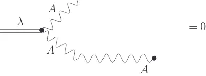
A λ
A
= 0
A
Figure 1. TheλAA-vertex contracted with a photon propagator vanishes.
(x1, x2)-plane, relation (2.30) has the following important consequence for the Feynman graphs: The combination of gauge boson propagator and λAA vertex is zero (see Fig.1).
Furthermore, it is impossible to construct a closed loop including a λAA-vertex without having such a combination somewhere. Hence, all loop graphs involving the λAA-vertex vanish. In particular, dangerous vacuum polarization insertions involving the additional Feynman rules (i.e. theλ-propagator, the mixed λA-propagator and the λAA-vertex) vanish. This is the reason, why the model is free of the most dangerous, i.e. the quadratic, infrared singularities, as pointed out by Slavnov [69] for the special case of nµ= (0,1,0,0).
2.3.2 Further generalization of the Slavnov trick
Now the question arises whether one can show the cancellation of IR singular Feynman graphs for a more general choice of Θµν and nµ. The answer is yes, but one has to impose stronger Slavnov constraints. The initial Slavnov constraint was Θ12F12+ Θ13F13+ Θ23F23= 0 and with
“stronger” we mean that each term in the sum should vanish separately. Upon imposing these stronger conditions one may write for the action (cf. [72]):
Sinv= Z
d4x
−1
4FµνF
µν+ 1
2ǫ
ijkF ijλk
,
with i, j, k ∈ {1,2,3}. This action looks like a 3 dimensional BF model coupled to Maxwell theory. As in the pure BF-case, the action has two gauge symmetries
δg1Aµ=DµΛ, δg2Aµ= 0,
δg1λk=−ig
λk,Λ
, δg2λk=DkΛ′.
Similar to the previous model, we have an additional bosonic vector symmetry of the gauge invariant action:
ˆ
δiA0=−Fi0, δˆiλj =ǫijkD0F0k, ˆδiAj = 0.
There is, however, a difference to the previous case: The additional vectorial symmetry is broken when fixing the second gauge symmetry δg2.
If one considers a space-like axial gauge fixing of the form7
Sgf = Z
d4xbniAi+d′niλi−¯cniDic−φn¯ iDiφ
,
the gauge fixed action is invariant under the linear VSUSY
δic=Ai, δiλj =−ǫijknk¯c, δib=∂i¯c,
δiΦ = 0 for all other fields,
7d′=d−ig¯ φ, c
in addition to the usual BRST invariance. The Ward identity describing the linear vector supersymmetry in terms of Zc at the classical level is given by
WiZc =
Z d4x
jb∂iδZ
c
δj¯c −
jcδZ c
δji A
+ǫijknjjλk
δZc δjc¯
= 0.
Hence, the same arguments as before show the absence of IR singular graphs. However, the model exhibits numerous further symmetries which have been discussed in [72].
One should also note, that a generalization to higher dimensional models is possible. For example ifλhad nindices the VSUSY would become
δic=Ai, δiλj1···jn =ǫikj1···jnn
k¯c, δ
ib=∂i¯c,
after appropriate redefinitions of Lagrange multipliers.
In conclusion, one can state that Slavnov-extended Yang–Mills theory can be shown to be free of the worst infrared singularities, if the Slavnov term is of BF-type. Furthermore, supersym-metry, in the form of VSUSY, seems to play a decisive role in theories which are not Poincar´e supersymmetric. Another open question is what role the VSUSY plays with respect to UV/IR mixing in topological NCGFT in general.
However, a general proof of renormalizability for this type of models is still missing. Further-more, the Slavnov-extended models have a major drawback: The Slavnov constraint reduces the degrees of freedom of a gauge model (see [69]) and hence it seems that it does not describe non-commutative “photons”.
2.4 Models with oscillator term
To avoid the UV/IR mixing problem, several models which involve an oscillator like counter term have been put forward. On the one hand such models break translation invariance due to the explicit x-dependence of the action, but on the other hand they in general show a much better divergence behaviour at higher loops or are even (in the case of the scalar Grosse–Wulkenhaar model) proven to be renormalizable. In the following, we will present the Grosse–Wulkenhaar model followed by three gauge models based on similar ideas.
2.4.1 The Grosse–Wulkenhaar model
In 2004, the first renormalizable non-commutative scalar field model (in Euclidean R4
θ) was
introduced by H. Grosse and R. Wulkenhaar [28] (for a Minkowskian version see reference [172]). Their trick was to add a harmonic oscillator-like term to the action
S[φ] = Z
d4x
1
2∂µφ ⋆ ∂µφ+ µ20
2 φ ⋆ φ+ Ω2
4 (˜xφ)⋆(˜xφ) + λ
4!φ ⋆ φ ⋆ φ ⋆ φ
, (2.31)
with ˜xµ= (Θµν)−1xν(Θµνconstant and antisymmetric). This action cures the infamous UV/IR
mixing problem. Indeed, for the bad IR-behaviour found in the na¨ıve model (triggered by the kinetic part of the action), the oscillator term acts as a sort of counter term. By exchanging ˜
x↔p one can see that the action stays form invariant:
S[φ;µ0, λ,Ω]7→Ω2S
φ;µ0 Ω,
λ Ω2,
1 Ω
.
The propagator of the model is the inverse of the operator (−∆ + Ω2x˜2+µ20), and is called the Mehler kernel [27]. It takes the form
KM(x, y) =
∞ Z
0
dα 1
4π2ωsinh2αe
−41ω(u2cothα
2+v2tanh
α
2)−ωµ20α,
withω= Ωθ,u=x−y being ashort variable andv=x+ybeing along variable. This notation has been introduced by V. Rivasseau et al. [173]. They confirmed the renormalizability of the model by making use of a technique called Multiscale Analysis, additionally to the renormaliza-tion proof of H. Grosse and R. Wulkenhaar which has been given in the matrix base employing the Polchinski approach.
The Mehler kernel features a damping behaviour for high momenta (UV) as well as for low momenta (IR). One can see this by comparison with the heat kernel, which is the inverse of H0 =−∆ +µ20 and has the form
H0−1 = ∞ Z
0
dα 1
16π2α2e
−(x+2αy)2−µ2 0α.
Forµ0 = 0, one finds the well-known form of the undamped propagator after integrating overα
H0−1 = 1 8π2(x−y)2.
When setting y = 0 andµ0 = 0 in the Mehler kernel, one can perform the integration over the
auxiliary Schwinger parameter and obtain
KM(x) =
e−x4ω2
π2x2,
which shows that the Mehler kernel has a much stronger convergence behaviour for large values of x, corresponding to small values of p. However, the price to pay seems to be that trans-lation invariance is broken, which can be seen directly in the action, because of the explicit x-dependence of the oscillator term ˜x2φ2. Recently, as discussed in Section 2.4.4, it has been shown that this term can be interpreted as a coupling to the curvature of a background space, giving it a nice geometrical interpretation.
The renormalizability of the model can also be beautifully illustrated by a quick glance at the beta function for λ, which can be found for example in [174]. In contrast to the na¨ıve scalar model (without oscillator term) the beta function becomes constant for high energies. Hence it does not diverge, and is therefore free of the Landau ghost problem [175,176,177].
2.4.2 Extension to gauge theories
The aim is to obtain propagators for gauge models with a damping behaviour similar to the Mehler kernel in the scalar case. Since an oscillator term Ω2x˜2A2 is not gauge invariant, there
are more or less two possible ways to construct the model: either one adds further terms in order to make the action gauge invariant (which will be discussed in the following section) or one views the oscillator term as part of the gauge fixing. H. Grosse, M. Schweda and one of the present authors (D. Blaschke) put forward a model which follows the latter approach [34]. The action is given by
Sinv=
The gauge fieldAµtransforms under the non-commutative generalization of aU(1) gauge
trans-formation which is infinite by construction of the non-commutative algebra. Once more, we denote the gauge group by U⋆(1) in order to distinguish it from the commutative U(1) gauge
group.
The multiplier fieldb implements a non-linear gauge fixing8:
δΓ(0)
The fieldecµis an additional multiplier field which guarantees the BRST-invariance of the action.
The BRST-transformations are given by
sAµ=Dµc=∂µc−ig
Since ecµ transforms into ˜xµ, the part of the action including the Lagrange-multiplier field ecµ
exactly cancels with Sm under the application of the BRST-operator s onto the whole action.
With these BRST transformations the action (2.32) can be written in the following beautiful form:
Feynman rules. When we assume Θµν to be antisymmetric and constant, i.e.
(Θµν) =ε
as defined at the beginning of Section 2, the following property holds:
Aµ⋆,x˜µ = 2˜xµAµ,
which can be directly verified by inserting the definition of the star product (2.2). It is therefore possible to reduce the bilinear parts of the action to one single star. The latter can be removed
by the cyclic permutation property of the star product (2.3), and therefore the non-interacting part of the action is the same as in an undeformed model. Hence the propagators are more or less just the Mehler kernels, like in the scalar case. In momentum space they are given by
GAAµν (p, q) = (2π)4KeM(p, q)δµν, Gcc¯(p, q) = (2π)4KeM(p, q),
with the Mehler kernel in momentum representation
e
The ecbc-vertex involving the multiplier field ecµ does not contribute to Feynman diagrams
since a propagator connecting to that field does not exist. Similarly, a propagator does exist forb, but the corresponding vertex as stated do not contribute to loop diagrams. Hence, we will omit the related Feynman rules.
The vertices following from the action are just the usual non-commutative ones, as can be found for example in [129]. Equipped with the complete Feynman rules we can start deriving a power counting formula to estimate the worst degree of divergence of our graphs, which via UV/IR mixing is directly related to the degree of non-commutative IR divergence. We will not give a detailed derivation here but instead quote only the final result. (For further details we refer the interested reader to [35].) Given the number of external legs for the various fields (denoted by Eϕ, ∀ϕ ∈ {Aµ, b, c,¯c,ecµ}) the degree of UV divergence for an arbitrary graph in
4-dimensional space can be up-bounded by
dγ= 4−EA−Ec/c¯−Eec−2Eb. (2.35)
This bound, however, represents merely a crude estimate. The true degree of divergence can (for certain graphs) be improved by gauge invariance. For example, for the one-loop boson self-energy graphs the power counting formula would predict at most a quadratic divergence, but gauge invariance usually reduces the sum of those graphs to be only logarithmically divergent. In our case we will show, however, that this does not happen due to a violation of translation invariance. The corresponding Ward identity will be worked out more explicitly in the next subsection.
Symmetries. In this subsection, we will take a closer look at the Ward identities (describing translation invariance) and the Slavnov–Taylor identities (describing BRST invariance). Every symmetry in general implies a conservation operator that gives zero when applied to the action. In the case of the BRST symmetry this is s. Regarding s as a total derivation of Γ(0) we can
write
By introducing external sources ρµand σ forsAµand sc, respectively
Γ = Γ(0)+ Γext, Γext= Z
d4x(ρµ⋆ sAµ+σ ⋆ sc) ,
and making use of (2.33) we can write the Slavnov–Taylor identity in a more convenient form:
∂µ = x˜
µ·
Figure 2. Ward identity replacing transversality.
+
Figure 3. Tadpole graphs.
To arrive now at the Ward identity describing translation invariance, one has to take as usual the functional derivative of the Slavnov–Taylor identity with respect toAρ andc. One immediately
recognizes that the ˜xµ-term which originates from the oscillator term in the action gives an
additional contribution. The usual translation invariance is explicitly broken:
∂µz δ
Graphically this can be depicted as shown in Fig. 2.
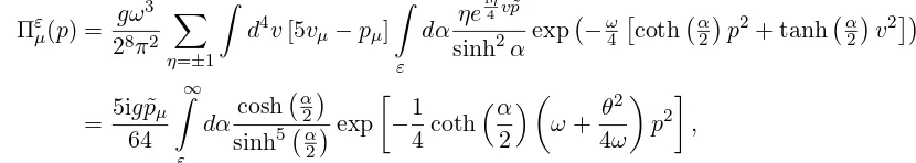
Loop calculations. The simplest graphs one may construct are the (one-point) tadpoles, consisting of just one vertex and one internal propagator. They consist of two graphs which are depicted in Fig.3. According to the Feynman rules, their sum is straightforwardly given by
Πµ(p) = 2ig
We may now transform to “long and short” variables
u=k−k′, v=k+k′ ⇒ k= v+u
2 , k
′ = v−u 2 ,
with functional determinant 161. Moreover, we make use of
sin
and plug in the explicit expression for the Mehler kernel (2.34). Altogether this leads to
Πεµ(p) = gω
Na¨ıvely, one could simply integrate out α and discover a divergence structure of higher degree than expected, since it still contains a “smeared out” delta function. To make this clear, consider the usual commutative propagator, which depends on a second momentum only through a delta function, i.e.G(k, k′)∝G(k)δ4(k−k′). In the present case, due to the breaking of translational invariance, the delta function is replaced by something which might be described by a smeared out delta function, which is contained in the Mehler kernel, and hence one cannot simply split that part off. However, by integrating over one external momentum one can extract the divergence one is actually interested in. In some sense one can interpret this procedure as an expansion around the usual momentum conservation. This is the general procedure we will use to calculate the Feynman graphs. The 1-point tadpoles however are an exception: since they have only one external momentum, integrating the latter out would equally mean to setp= 0. (One can see this by noticing that the integrand is antisymmetric in p, and the integration over the symmetric interval from −∞ to ∞ would thus give zero.) With this procedure we would just hide the divergences. In conclusion, one can state that the integration over an external momentum is applicable for graphs with more than one external leg.
For the 1-point graphs, we use the trick of coupling an external field to the graph and expanding it around p= 0:
Z d4p
After smearing out the graph by coupling it to an external field, an integration overpis allowed. All terms of even order are zero for symmetry reasons. Of the other terms, we now show that only the first two, namely orders 1 and 3, diverge in the limit ε→0:
• order 1: With the external field, we obtain a counter term of the form
• order 3: We get the counter term
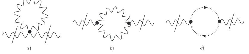
a) b) c)
Figure 4. Gauge boson self-energy – amputated graphs.
describe nature, we must have started with a wrong vacuum. Furthermore, since we get addi-tional counter terms of mathematical structure which were not initially present in the original action, we certainly need a new theory. Apparently this is the case here because equations (2.37) and (2.38) reveal counter terms linear inAµ. Ultimately this means that we will have to consider
a whole new model, which will be the induced gauge theory, but more on that in Section 2.4. Two-point functions at one loop level. Here we analyze the divergence structure of the gauge boson self-energy at one-loop level. The relevant graphs are depicted in Fig. 4.
As explained in the previous paragraph, we do not need to couple an external field and expand around it in this case. The notion of long and short variables has proven to be very useful and we will use it again here. In order to be able to calculate the three graphs, we use the following simplifications:
• For the cosine we use
cos
kp˜ 2
= X
η=±1
1 2exp
iη
2kp˜
.
• We approximate the hyperbolic functions of the Mehler kernel:
cothα 2
≃ 2
α, tanh α
2
≃ α
2, sinh(α)≃α
for the dangerous regionα= 0, where the kernel has a quadratic pole, in order to extract the divergent parts of our Feynman graphs.
• We will, in addition to the inner momenta, integrate over the external momentum p′ in order to reveal the divergence structure of the general result without the “smeared out delta function” of the Mehler kernel.
• For the parameter integrals α (one per Mehler kernel) we perform a useful change of variables, which can be found e.g. in [178, page 15].
In this form, we can easily sum up all three graphs Fig. 4a), b) and c). The sum yields the final result
Πdivµν(p) = g
2δ
µν 1−34Ω2
4π2ω ε1 +Ω2 4
3 +
3g2δ
µνΩ2
8π2p˜21 +Ω2 4
2 +
2g2p˜
µp˜ν
π2(˜p2)21 +Ω2 4
2
+ logarithmic UV divergence. (2.39)
In the limit Ω→0 (i.e. ω→ ∞), this expression reduces to the usual transversal result
lim
Ω→0Π div
µν(p) =
2g2 π2
˜ pµp˜ν