E l e c t ro n ic
J o u r n
a l o
f P
r o b
a b i l i t y
Vol. 7 (2002) Paper no. 21, pages 1–21. Journal URL
http://www.math.washington.edu/~ejpecp/ Paper URL
http://www.math.washington.edu/~ejpecp/EjpVol7/paper21.abs.html
THE NOISE MADE BY A POISSON SNAKE
Jon Warren
Department of Statistics, University of Warwick Coventry, CV4 7AL, United Kingdom
Abstract: The purpose of this article is to study a coalescing flow of sticky Brownian motions on [0,∞). Sticky Brownian motion arises as the weak solution of a stochastic differential equation, and the study of flow reveals the nature of the extra randomness that must be added to the driving Brownian motion. This can be represented in terms of Poissonian marking of the trees associated with the excursions of Brownian motion. We also study the noise, in the sense of Tsirelson, generated by the flow. It is shown that this noise is not generated by any Brownian motion, even though it is predictable.
Keywords and phrases: stochastic flow, sticky Brownian motion, coalescence, stochastic differential equation, noise.
AMS subject classification (2000): 60H10, 60J60.
1
INTRODUCTION
Suppose that ¡
Ω,(Ft)t≥0,P
¢
is a filtered probability space satisfying the usual conditions, and that¡
Zt;t≥0¢
is a continuous, adapted process taking values in [0,∞) which satisfies the stochastic differential equation
Zt=x+ Z t
0
1(Zs>0)dWs+θ Z t
0
1(Zs=0)ds, (1.1)
where ¡
Wt;t ≥ 0¢
is a real-valued Ft-Brownian motion and x ≥ 0 and θ ∈ (0,∞) are constants. We say that Z is sticky Brownian motion with parameter θ started from x. Sticky Brownian motion arose in the work of Feller [6] on strong Markov processes taking values in [0,∞) that behave like Brownian motion away from 0. The parameterθdetermines the stickiness of zero: the cases (which we usually exclude) θ = 0 and θ =∞ correspond respectively to Brownian motion absorbed or instantaneously reflected on hitting zero. For
θ ∈ (0,∞) sticky Brownian motion can be constructed quite simply as a time change of reflected Brownian motion so that the resulting process is slowed down at zero, and so spends a non-zero amount of (real) time there. However here our interest will be focused on it arising as a solution of the stochastic differential equation (1.1). This equation does not admit a strong solution, in order to construct Z it is necessary to add to the driving Brownian motion W some extra ‘randomness’. The nature of this randomness was first investigated in [15]. More recently it has been shown (Warren, [16], and Watanabe, [17], following Tsirelson, [13]) that the filtration (Ft)t≥0 cannot be generated byany Brownian
motion.
The main object of study in this paper is a coalescing flow on R+ which we denote by
¡
Zs,t; 0 ≤s≤t <∞¢
, where eachZs,t is an increasing function from R+ to itself. We may
describe the flow rather informally in terms of the motion of particles. For any t and x
the trajectoryh7→Zt+h(x) describes the motion of a particle which starts at timetfrom a positionx. We shall be concerned with a flow in which this motion is determined by a sticky Brownian motion. Away from zero, particles move parallel to each other- which means that the SDEs (similar to equation (1.1)) which describe their trajectories are all driven by the same Brownian motion W. Particles collide while visiting zero and thereafter they move together- and the mapZs,t is typically neither injective nor surjective.
The stochastic differential equation (1.1) was studied in [15]. There it was shown that the solution is weak, and that for each t, assuming Z0 = 0, the conditional distribution of Zt given the entire path of the driving Brownian motion W is given by:
P¡Zt≤z|σ(Ws;s≥0) ¢
= exp(−2θ(Wt+Lt−z)) z∈[0, Wt+Lt], (1.2) whereLt= sups≤t(−Ws).
An interpretation of (1.2) was given in [15] which we can summarise loosely as follows. Define a processξ via
ξt=Wt+ sup s≤t ¡
−Ws¢ t≥0. (1.3)
ξ is then a Brownian motion reflected from zero. Each excursion ofξ from zero gives rise to a rooted tree. Each timet determines a path in the tree corresponding to the excursion of
ξ which straddlest. This path starts from the root of the tree and is of lengthξt. If times
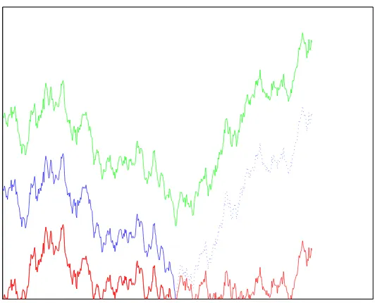
Figure 1: The trajectories of three particles in a typical realization of the flow. The upper particle never hits zero and its trajectory is a translate of the driving Brownian motion. The middle particle has started from a critical height- it just hits zero and from then on follows the same trajectory as the lowest particle which was started from zero. The dotted line shows the path that would be taken by the middle particle if the boundary were not sticky.
we add marks to these trees according to a Poisson point process of intensity 2θ. We can then construct the sticky Brownian motionZ from these marked trees via, for eacht≥0,
Zt= (
0 if the path corresponding tot is not marked,
ξt−ht otherwise,
(1.4)
whereht is the distance along the path corresponding tot from the root to the first mark. Notice that not all the marks carried by the trees are used in constructing the processZ in this way.
In this paper the description of the previous paragraph is extended to the flow¡
Zs,t;s≤t¢ of sticky Brownian motions. By replacing the single sticky Brownian motion by an entire flow we make natural use of all the marks on the trees. A discrete version of the correspondence between a flow and a family of marked trees is illustrated in Figures 2 and 3.
Section 2 of the paper details the construction of the flow. We begin with a process ¡
Xt;t≥
0¢
, taking values in R∞ which solves an infinite family of stochastic differential equations. FromX we are able to construct the flow in a pathwise manner.
In Section 3 we show that a generalization of (1.4) holds for the processX. There exists a family of marked trees such that the componentsX(1), X(2), . . . , X(k), . . . ofX satisfy
Xt(k)= (
0 if the path corresponding tot carries fewer thank marks,
ξt−h(tk) otherwise,
(1.5)
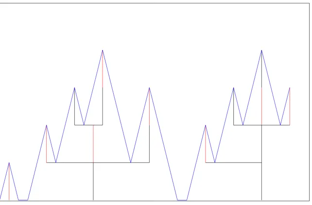
Figure 2: Three typical trajectories for a discrete version of the flow. As in Figure 1 the dashed line is to illustrate the effect of the sticky boundary.
closely related construction involving Poisson marking of trees is described by Aldous and Pitman [3].
In the final section we consider the flow as a noise, in the sense of Tsirelson [11] and [12]. The flowZ has independent stationary increments, in that, for any 0≤t0 ≤t1 ≤. . .≤tn the random mapsZt0,t1, Zt1,t2, . . . Ztn−1,tn are independent and fors≤tandh >0 the maps
Zs,t andZs+h,t+h have the same distribution. We will writeFs,tfor theσ-algebra generated by ¡
Zu,v;s ≤ u ≤ v ≤ t ¢
. Following Tsirelson the doubly indexed family ¡
Fs,t;s ≤ t ¢
is called a noise. It is a non-white noise because, as we shall see, there is no Brownian motion whose increments generate it.
2
CONSTRUCTING THE FLOW
Let R∞ denote the space of real-valued sequences with the product topology. We will denote (for reasons shortly to become clear) the canonical process on the spaceC¡
R+,R∞
. Often we use the notation
Xt(0)=Wt+ sups≤t(−Ws).
Theorem 1. Let θ ∈ (0,∞). There exists a unique probability measure P on C¡
R+,R∞¢
such that the canonical process ¡
Xt;t≥0)satisfies the following.
• The first component, W, is a Brownian motion starting from 0 with respect to the filtration generated by X.
• Fork≥1, the processes X(k) are non-negative and the following SDEs are satisfied: Xt(1)=
Proof. We begin by proving that P is unique. Let P(n) denote the restriction of P to the
σ-algebra F(n) generated by W, X(1), . . . , X(n). Since the union of such σ-algebras is an
algebra generating the entire Borel σ-algebra, it suffices to prove that eachP(n) is unique. Let, for any k≥1,
and denote their right-continuous inverses by α(k) and α(k+) respectively. We shall see
shortly thatA(∞k) =A∞(k+) =∞ with probability one, and so we may define, for any k≥1
V, Theorem 1.9). Hence if we can recover W, X(1), . . .,X(n) from them, the measure P(n)
will be determined uniquely. Now, we may write,
Xt(k) =B(k+)
A(tk+)+θA
(k)
t .
Since the lefthandside is non-negative, and A(k) grows only when it is zero, we recall that
the Lemma of Skorokhod (see [9], Chapter VI, Lemma 2.1) tells us that,
θA(tk)=S(k)
A(tk+), where we denote,
Su(k)= sup h≤u ¡
−Bh(k+)¢
.
Note that,
At((k−1)+)=At(k)+A(tk+)= 1
θS
(k)
A(tk+)+A
(k+)
t .
When k = 1 we may take the lefthandside to be given by A(0+)t = t. We can now check the earlier claim thatA(∞k)=A(∞k+) =∞. If, for some k, we had A(∞k+) <∞ then repeated
application of the preceeding equation would give A(0+)∞ < ∞- a falsehood. So we deduce
thatA(∞k+)=∞, but then we haveA∞(k)=S∞(k)/θ=∞ with probability one.
Denote by σ(k) the inverse of the continuous, strictly increasing function:
u7→ 1 θS
(k)
u +u. Then, we find that,
(*) Bt((k−1)+) =B(k+)
σ(tk) +B
(k)
t−σ(tk), and
(**) A(tk+)=σ(k)
A((tk−1)+)
.
These two relations hold even fork= 1 provided that we takeB(0+)t =Wtand A(0+)t =t. Now for any fixednwe can use (*) to recoverB(0+),. . .,B(n+) fromB(1),. . .,B(n),B(n+).
Moreover we can then use (**) to obtain A(1+), . . . , A(n+), and then, finally, we obtain
X(1), . . . , X(n), since
(***) Xt(k)=B(k+)
A(tk+)+S
(k)
A(tk+).
More precisely we are able to write, for any finite set of timest1, t2, . . . , tm, the m(n+
1)-tuple Wt1, X
(1)
t1 , . . . , X
(n)
t1 , . . . , . . . , Wtm, X
(1)
tm, . . . , X
(n)
tm as a jointly measurable function of
B(1),. . . ,B(n),B(n+), and this determinesP(n) on a generatingπ-system. This completes the proof of uniqueness.
To prove existence we construct, for each n the probability measure P(n) on ³
C¡
R+,R∞
¢
sequence of measures is consistent (by virtue of the uniqueness property just obtained), and we may take Pto be its projective limit.
Fix n ≥ 1. To construct W, X(1), . . . , X(n) we start with n+ 1 independent Brownian
motions denoted byB(1), . . . , B(n), B(n+)and, as in the proof of uniqueness, define, in turn,
B((n−1)+), B((n−2)+), . . . B(0+), by means of (*). Then, starting fromA(0+)t =t, we define via (**) increasing processes A(1+), . . . A(n+), and finally we use (***) to obtain the processes
X(1), . . . , X(n) and take W = B(0+). We must show that the processes so constructed
satisfy the appropriate SDEs, and thatW is a Brownian motion. We do so via an inductive argument.
Call the common valueA(tk) and note that this identifies the second term on the righthand-side of (***). It remains to identify the first term as a stochastic integral against W. Write Wt = Mt+Nt where Nt = B(k+) The first integral must be identically zero because the zero set of the integrand supports the measuredMtdMtwhile the second integral is simplyB(k+)
A(tk+)
. Applying the above arguments fork= 1,2, . . . , n we deduce that all the necessary SDEs are satisfied.
The remaining issue is to verify thatW is a Brownian motion with respect to the filtration generated by W, X(1), . . . , X(n). Suppose thatB(k+) is a Brownian motion with respect to
But B((k−1)+), having quadratic variation process t, is thus a G(k−1)
t -Brownian motion by L´evy’s characterization. If we apply this argument successively, firstly for k= n and G(n)
the natural filtration of B(n+) then for k = n−1, . . . ,2,1 we find that W = B(0+) is a
G(0)-Brownian motion. But the processesW, X(1), . . . , X(n)are allG(0)-adapted and we are
finished.
In the following we will work with the probability space given by this theorem, and with respect to the filtration denoted by ¡
Ft ¢
t≥0, the smallest right-continuous and P-complete
filtration to whichXis adapted. Since we want to construct the flowZfromXin a pathwise manner we need to restrict ourselves to a subset of C¡
R+,R∞
¢
on which X is sufficiently well behaved. Our first task is to identify such a subset.
For eachtlet ˆNtdenote the smallestk≥0 such thatXt(k+1) is zero, or be infinity if no such
k exists. As we shall see the process ¡ˆ
Nt;t ≥ 0 ¢
must be treated with respect; it is very singular. For anys≤tlet ˆNs,t = inf{Nˆh :s≤h≤t}.
Lemma 2. The following hold with probability one.
• For every t ≥ 0 the sequence ¡
Proof. We continue to use notation as introduced in the proof of the preceeding theorem. We will show that, for allu and k,
for all t, and with equality only if both sides are 0. Recall that above, is constant on each component of the set
and hence
occurring fort belonging toS is zero.
Let us prove the second assertion of the lemma: that ˆNs,t is finite for all s < t with probability one. On applying Itˆo’s formula we find that, for anyλ >0, and any k≥1,
exp© is a bounded martingale. Taking expectations, and lettingt→ ∞we calculate that:
E
we deduce that, with probability one, for all t,
∞
has measure zero, and a complement dense inR+.
It is not true that with probability one ˆNtis finite for allt. For eachk, the set{t: ˆNt> k} is open and dense, and thus by virtue of Baire’s Category Theorem the set{t: ˆNt=∞}= ∩k{t: ˆNt> k}is dense.
We now describe a result that will eventually lead to the independent increments property of the flow. If W(1) and W(2) are independent Brownian motions starting from zero and
t0 some fixed time, then the process W defined by
Wt= (
Wt(1) ift≤t0,
and obtained by splicing¡ a Brownian motion. A more complicated procedure is given in the following lemma which generalizes this construction.
Lemma 3. Suppose we are given two independent processesX(1)andX(2)each distributed according to the law given by Theorem 1. Fix somet0, and construct a processX as follows.
For each x≥0 let
Then the process X is also distributed according to the law determined by Theorem 1.
Proof. As remarked previouslyW is a Brownian motion, and indeed it is a Brownian motion with respect to the filtration generated by X since any incrementWu−Wt is independent of ¡
Xs; 0 ≤ s ≤ t¢
. Note also that the times Tk are stopping times with respect to this filtration.
( this may be empty-it does not matter). Fors belong-ing to this interval we have Xs(1)> Xs(2) > . . . > Xs(m)>0, and so, for anyk=m+r > m,
Notice how to recover ¡
Xt(1); 0≤t≤t0
¢ and ¡
Xt(2);t≥0¢
fromX. The former is simply the restriction of X to times t ≤ t0. While W(2) is given by Wt(2) = Wt+t0 −Wt0 the
recovery of X(r)(2) for r ≥ 1 is more involved. Since T
m = inf{t ≥ t0 : Xt(m) = 0} if
t0 ≤t < Tm thenXt(m)>0 and ˆ
Nt= inf{k:Xt(k+1)= 0} ≥m. Also ˆNTm+1 ≤m sinceX
(m+1)
Tm+1 = 0, and so fort∈[Tm+1, Tm) we have
ˆ
Nt0,t= inf{Nˆh :t0≤h≤t}=m.
Consequently we have
X( ˆNt0,t+r)
t =X
(r)
t−t0(2) r≥1.
The special caser = 1 deserves attention:
X( ˆNt0,t+1)
t =X
(1)
t−t0(2)
which as t≥t0 varies is a sticky Brownian motion starting from zero at timet=t0. This
is the key to the construction of the flow fromX.
Theorem 4. Define for all 0≤s < t <∞, functions Zs,t:R+7→R+, by
Zs,t(x) = (
Xt( ˆNs,t+1) for 0≤x≤Us,t,
Wt−Ws+x for Us,t< x.
where sups≤h≤t ¡
Ws−Wh ¢
is denoted by Us,t. We complete the definition ofZ by takingZt,t
to be the identity for all t.
Then with probability one Z possesses the properties of a flow: for all 0≤s≤t≤u <∞, Zs,u=Zt,u◦Zs,t.
For all x∈R+ and any s≥0,
t7→Zs,t(x) is continuous as t≥svaries. Moreover this trajectory satisfies the stochastic differential equation,
Zs,t(x) =x+ Z t
s
1(Zs,u(x)>0)dWu+θ Z t
s
1(Zs,u(x)=0)du.
The doubly indexed process ¡
Zs,t; 0 ≤ s ≤ t < ∞¢
has independent and stationary in-crements: for any 0 ≤ t0 ≤ t1 ≤ . . . ≤ tn the random maps Zt0,t1, Zt1,t2, . . . Ztn−1,tn are
independent and fors≤tandh >0 the mapsZs,t andZs+h,t+h have the same distribution.
Proof. Fix s < t < u. We evaluate the composition Zt,u ¡
Zs,t(x)¢
in four distinct and exhaustive cases. First note the following estimate,
(*) Xt( ˆNs,t+1)≤Wt−Ws+Us,t.
(**) Nˆs,u= min ©ˆ
Ns,t,Nˆt,u ª
.
Let
T = inf{h≥t:Xh( ˆNs,t+1)= 0}.
CASE 1. Suppose that x > Us,t and Wt −Ws +x > Ut,u. These conditions may be interpreted as saying that a particle started from x at time s does not reach zero by time
u. Then,
Zt,u¡Zs,t(x)¢=Zt,u¡Wt−Ws+x¢ =Wu−Ws+x. CASE 2. Suppose thatx ≤Us,t and X( ˆ
Ns,t+1)
t > Ut,u. This time the particle starting from
xat time shits zero before timetbut then does not visit zero during the interval [t, u]. We have T > u, and so for 1≤k≤Nˆs,t+ 1, andh∈[t, u], we have Xh(k) >0, so (recall always Lemma 2) ˆNt,u≥Nˆs,t+ 1 and whence by virtue of (**) ˆNs,u= ˆNs,t and,
Zt,u ¡
Zs,t(x)¢ =Zt,u
¡
Xt( ˆNs,t+1)) =Xt( ˆNs,t+1)+Wu−Wt=Xu( ˆNs,t+1) =Xu( ˆNs,u+1).
CASE 3. Suppose that x≤Us,t and Xt( ˆNs,t+1)≤Ut,u. The particle starting from xat time
svisits 0 during both intervals [s, t] and [t, u]. Then,t≤T ≤u, and so ˆNt,u ≤Nˆs,t, whence, using (**) again, ˆNt,u= ˆNs,u. Thus,
Zt,u¡Zs,t(x)¢=Zt,u¡Xt( ˆNs,t+1)) =X
( ˆNt,u+1)
u =Xu( ˆNs,u+1).
CASE 4. Suppose thatx > Us,tandWt−Ws+x≤Ut,u, so that the particle starting fromx at timesvisits 0 during the interval [t, u] but not during [s, t]. Combining these inequalities with that denoted by (*) above, Xt( ˆNs,t+1) ≤Ut,u, so t ≤T ≤u and and we may argue as for the preceding case that ˆNt,u = ˆNs,u. Thus
Zt,u¡Zs,t(x)¢=Zt,u¡Wt−Ws+x) =Xu( ˆNt,u+1) =Xu( ˆNs,u+1).
Finally note that x > Us,u if and only if CASE 1 holds, and so we have demonstrated the required composition property.
ConstructXas in the preceding lemma from two independent copiesX(1) andX(2) taking the splicing time t0 to be equal tos, then we commented following Lemma 3 that
Xt( ˆNs,t+1) =Xt(1)−s(2),
and it is also the case that
Us,t= sup
0≤h≤t−s ¡
−Wh(2)¢
=U0,t−s(2).
By virtue of Lemma 2 we can now deduce equation (*) above since
Xt(1)−s(2)≤Xt(0)−s(2) =Wt−Ws+Us,t.
We can also prove that Z has stationary, independent increments from this splicing. The mapZs,t can be written in terms ofX(2) as
Zs,t(x) = (
Xt(1)−s(2) for 0≤x≤U0,t−s(2),
Thus Zs,t is determined from X(2) in the same way that Z0,t−s is determined from X and so has the same law as Z0,t−s. The construction also shows that Zs,t is independent of ¡
Zu,v; 0≤u≤v≤s¢
, this being determined byX(1).
Finally note thatt7→Xt(1)−s(2) is fort≥sa sticky Brownian motion starting from zero and this is the same as t7→Zs,t(0). More generally
Zs,t(x) = (
x+Wt−Ws s≤t≤τ,
Zs,t(0) t≥τ
whereτ = inf{t≥s:x+Wt−Ws ≤0}, from which we may easily deduce thatt7→Zs,t(x) is, for t≥s, a sticky Brownian motion starting at time sfrom x, and that this trajectory satisfies the SDE as claimed.
Lemma 5. We may recover the processX from the flow: for each t,
©
Zs,t(0) : 0≤s < t ª
=©
Xt(k):k≥1ª
.
Proof. To see this note first that the inclusion ©
Zs,t(0) : 0≤s < tª ⊆©
Xt(k):k≥1ª
.
follows from the very definition of Zs,t(0) as Xt(k) for some k. This inclusion is in fact an equality as the following argument shows. For eachk≥1 let
g(tk)= sup{s≤t:Xt(k)= 0},
then Xh(k) = Wh −Wg(k)
t
for h ∈ [gt(k), t]. Now, using the fact that the Xt(k) take distinct values for differentk unless equal to zero, we see that:
ˆ
N
gt(k),t
= inf©
r :Xh(r+1) = 0 for some h∈[g(tk), t]ª
=k−1,
unless gt(k)=t and Xt(k) = 0. It follows that Zg(k)
t ,t
(0) =Xt(k) for allk such that Xt(k)>0. Finally note that if, for somekwe haveXt(k)= 0 thenZs,t(0) = 0 also forssufficiently close tot. Thus regardless of the value ofXt(k)there is always somes < twithZs,t(0) =Xt(k). The maps Zs,t were expected to have a simple form on the basis of the verbal description given in the introduction. For an initial position x sufficiently large the motion is simply a ‘translate’ of W. Whereas for all values x less than or equal to some critical level, the corresponding particles have reached zero between times s and t and coalesced. We can identify the mapZs,t with a point
¡
Xs,t, Us,t, Vs,t ¢
∈R3+ where
Us,t= sup s≤h≤t
(Ws−Wh), (2.1a)
Vs,t= sup s≤h≤t
(Wt−Wh), (2.1b)
Xs,t=Zs,t(0). (2.1c) Notice that, equation (*) from the proof of Theorem 4 can be written
and in fact this holds simultaneously for all s≤twith probability one. When we compose such maps we obtain via this identification a semigroup on ©
(x, u, v) ∈ R3+ : x ≤ v}; the
mapz associated with (x, u, v) being
z(ξ) = (
x ifξ ≤u,
v−u+ξ ifξ > u. (2.3)
Thus when we compose the maps associated with z1 = (x1, u1, v1) and z2 = (x2, u2, v2) we
obtain the map associated withz3 = (x3, u3, v3) =z2◦z1 where
u3 =u1+ (u2−v1)+ (2.4a)
v3 =v2+ (v1−u2)+ (2.4b)
x3 =x21(u2≥x1)+ (x1+v2−u2)1(u2<x1). (2.4c)
Using this identification of each mapZs,twith a point inR3+we can investigate the continuity
of (s, t) 7→ Zs,t. Discontinuities are caused by jumps in Xs,t which in turn are caused by jumps in ˆNs,t. For a pair of timess0< t0 letk= ˆNs0,t0+ 1. Then if r < k,X
(r)
h >0 for all
h∈[s0, t0], and in fact by continuity allhin some larger open interval containing [s0, t0]. If
there exists h0 ∈(s0, t0) with Xh(k0)= 0 then ˆNs,t = ˆNs0,t0 for all pairs s, t sufficiently close
tos0, t0. The alternative is that the onlyh∈[s0, t0] such thatXh(k)= 0 areh=s0 orh=t0
or both. In these cases (s, t)7→ Nˆs,t has a simple discontinuity at (s0, t0). However not all
such discontinuities in ˆN cause discontinuities in (s, t) 7→ Xs,t = Zs,t(0). It is only if the only h∈[s0, t0] such thatXh( ˆNs0,t0+1) = 0 ish=s0 thatXs,t has a point of discontinuity at (s0, t0) which is of the form:
lim
h,k→0,h≥0Xs−h,t+k exists and equals Xs,t (2.5a)
lim
h,k→0,h>0Xs+h,t+k exists . (2.5b)
Another place to worry about the continuity of (s, t)7→Xs,t is on the diagonal s=t. Here the behaviour of (s, t) 7→ Nˆs,t is particularly bad. But the inequality Xs,t ≤ Vs,t assuages our concerns.
3
LOOKING AT THE FLOW BACKWARDS
In this section we study the flow¡
Zs,t;s≤t¢
by fixingtand lettingsdecrease. This reveals certain random variables which have a Poisson distribution and leads to a verification of the description of the R∞-valued process X in terms of marked trees which was given in the introduction. Recently Watanabe [19] has also made a similar study of the flowZ in which the dual flow is described in terms of elastic Brownian motions. Let us define, for s < t, a random set Ξs,t via
Ξs,t={Zh,t(0) :s≤h < t}. (3.1) Recall from Theorem 4 or Lemma 5 that the flow Z is constructed from the R∞-valued processX in such a way thatZs,t(0) is equal toXt(k) for a certain random k. Thus
Ξs,t⊆ {Xt(k) :k= 1,2, . . .}, (3.2)
The principal result of this section is the description of the law of Ξs,t conditional on the driving Brownian motion¡
Wt;t≥0¢ .
Theorem 6. For fixed s < t, the law of Ξs,t conditional on ¡
Wt;t ≥ 0¢
is given, by the following.
• 0∈Ξs,t with probability one;
• Ξs,t\ {0} is distributed as a Poisson point process of intensity 2θ on(0, Vs,t].
In proving this theorem it is helpful to extend the flow to negative time. Thus suppose ¡
Zs,t;−∞ < s ≤ t < ∞¢
is a flow defined for all time with stationary independent incre-ments, and whose restriction to positive time is the flow constructed in Theorem 4. Suppose also that Z possess the regularity properties (2.5). As in the introduction let Fs,t be the
σ-algebra generated by ¡
Zu,v;s≤u≤v≤t¢ which we complete to contain all events with zero probability.
Lemma 7. Suppose thatT is a finite stopping time with respect to the filtration ¡ F−t,0
¢ t≥0
then
¡
Zs−T,t−T;−∞< s≤t≤0 ¢law
= ¡
Zs,t;−∞< s≤t≤0¢
,
and is moreover independent of F−T,0.
Proof. We mimic the usual proof of the strong Markov property. Suppose the stopping time
T only takes values in a discrete set of times, then, by virtue of the stationarity of the flow and the fact that F−∞,−ti and F−ti,0 are independent, the result holds forT. An arbritary
stopping time is the limit of a decreasing sequence of such elementary stopping times. Using this fact we deduce the result for an arbitrary finiteT noting that ash↓0, for anys≤t≤0,
Zs−(T+h),t−(T+h)→Zs−T,t−T,
by equation (2.5).
For a flow which is defined for all negative time we extend the driving Brownian motionW
to negative time by the device of considering the doubly indexed process ¡
Ws,t;−∞< s≤ t <∞¢
defined by
Ws,t=Zs,t(x) for sufficiently largex.
For non-negative s and t this is just the increment Wt−Ws of the Brownian motion W. The definitions ofUs,t and Vs,t can be extended to negative times via:
Us,t = sup h∈[s,t]
¡ −Ws,h
¢
and Vs,t = sup h∈[s,t]
¡
Wh,t ¢
(3.3)
We may also define a random set Ξ−∞,0 to be{Zs,0(0) :−∞< s <0}.
Lemma 8. Ξ−∞,0\ {0} is a Poisson point process on (0,∞) with intensity2θ and is
inde-pendent of ¡
Ws,t;−∞< s≤t <∞¢
.
Proof. For x ≥0 let −Tx = sup{s≤0 : Vs,0 > x}. Then x 7→ Tx is right-continuous, and each Tx is a¡F−t,0¢t≥0-stopping time by virtue ofF−t,0 being complete.
We define a right continuous counting process¡
N(x);x≥0¢ via
N(x) =n¡
wherenS counts the number of points belonging to the set S. Now fix somex and notice that V−Tx,0 =x. If−Tx≤s <0 then
Zs,0(0)≤Vs,0 ≤V−Tx,0=x.
On the other hand if s < −Tx then Zs,0(0) = Z−Tx,0 ◦Zs,−Tx(0), which is either equal to
Z−Tx,0(0) or strictly greater thanx. From this we deduce two facts. Firstly that
¡
On applying the previous lemma we deduce thatN is a process with independent identically distributed increments, and since it is constant except for positive jumps of size one, it must be a Poisson process of with some rate that remains to determine.
Before discussing the rate of N we first prove that it is independent of ¡
Ws,t;−∞ < s ≤ t < ∞¢
. In fact because of the independence of flow before and after time 0 it is enough to show that N is independent of ¡
Ws,t;−∞ < s ≤t ≤0¢
. It follows from Lemma 2 and stationarity that for each fixeds <0 with probability one, the strict inequality holds
Zs,0(0)< Vs,0.
Nevertheless there exist random s at which equality holds: the times −Tx for x ∈ Ξ−∞,0
in fact. By Fubini’s Theorem, with probability one, the Lebesgue measure of the set of these exceptional s for which equality holds is zero. Now consider an interval of the form [−Tx,−Tx−] for which Tx 6=Tx−= limǫ↓0Tx−ǫ. Forsbelonging to such an interval
Zs,0(0) =Z−Tx−,0◦Zs,−Tx−(0) =Z−Tx−,0(0).
This latter value cannot be equal to x, for if it was then Zs,0(0) = x = Vs,0 for all s in
the interval and the interval would then have to have length zero. Notice that if s <−Tx or −Tx− < s then Zs,0(0) cannot be equal to 0 either, and so we have shown that any x
such that Tx− < Tx cannot belong to Ξ−∞,0 and is not the time of a jump of the process
¡
N(x);x≥0¢
. Butx such thatTx−< Tx are exactly the local times at which the reflecting Brownian motion ¡
W−t,0 +V−t,0;t ≥ 0¢ makes excursions from zero. It follows from a
well-known property of Poisson processes (see [9], Chapter XII, Proposition 1.7) that N is independent of the Poisson point process of excursions from zero made by this reflecting Brownian motion and hence from the reflecting Brownian motion itself. Finally we note that we can recover ¡
Ws,t;−∞< s≤t≤0 ¢
from this reflecting Brownian motion and the proof of independence is complete.
where we have used the resolvent of Brownian motion and the fact that V0,t has the same law as |Bt|. This shows that β = 2θ.
Proof of Theorem 6. We have 0∈Ξs,t unless ˆNt =∞ which according to Lemma 2 occurs only for a set ofthaving Lebesgue measure zero. Thus by stationarity for any fixedsandt
the probability that 0∈Ξs,tis one. By Fubini’s Theorem it follows 0∈Ξs,twith probability one having conditioned onW ( except for a null set of possible values forW.)
We consider the extended flow defined for negative time. By stationarity and Lemma 8 Ξ−∞,t\ {0}={Zs,t(0) :−∞< s < t} \ {0}
is distributed as a Poisson point process with rate 2θ on (0,∞) and is independent of the white noise (Ws,t;s ≤ t) and hence of the Brownian motion (Wt;t ≥ 0) = (W0,t;t ≥ 0). Finally
Ξs,t= Ξ−∞,t∩[0, Vs,t], and Vs,t is measurable with respect toW.
Corollary 9. The law of Zs,t depends only on h=t−s and is given by ¡
Zs,t(0), Us,t, Vs,t ¢ law
= ¡
(U Rh−T)+,(1−U)Rh, U Rh ¢
(3.4)
where U is a variable uniformly distributed on [0,1], T is an exponential random variable with mean 1/(2θ), Rh is distributed as
√
hR1 for R1 the modulus of a standard Gaussian
variable in R3, and the three variables U, T and Rh are independent.
Proof. The marginal law of (Us,t, Vs,t) which depends just on the BMW is very well known see for example [20]. The exponentially distributed contribution describing the conditional law of Zs,t(0) is a consequence of Theorem 6 above, since Zs,t(0) > x if and only if Ξs,t contains a point in (x, Vs,t].
We turn now to an examination of the joint law of Ξ0,t1 and Ξ0,t2 when t1< t2. It is at this
point that the tree structure discussed in the introduction becomes evident.
Proposition 10. For fixed t1 < t2, the joint law of Ξ0,t1 \ {0} and Ξ0,t2 \ {0} conditional
on¡
Wt;t≥0¢
is given by the following.
1. IfV0,t1 ≤Ut1,t2 thenΞ0,t1\ {0} andΞ0,t2\ {0}are independent Poisson point processes
of intensity2θ on(0, V0,t1]and (0, V0,t2]respectively.
2. If V0,t1 > Ut1,t2 thenΞ0,t2 is composed of two pieces, one derived from Ξ0,t1, and the
other independent of it:
(a) the restriction ofΞ0,t2 to(Vt1,t2, V0,t2]is equal to the translation of the restriction
of Ξ0,t1 to (Ut1,t2, V0,t1]by Wt2 −Wt1, that is,
Ξ0,t2|(Vt1,t2,V0,t2]= (Wt2−Wt1) + Ξ0,t1|(Ut1,t2,V0,t1];
(b) the restriction of Ξ0,t2\ {0} to(0, Vt1,t2]and Ξ0,t1 \ {0} are independent Poisson
Proof. First observe that Ξ0,t1\{0}and Ξt1,t2\{0}are by virtue of Theorem 6, conditionally
onW, distributed as Poisson point processes of rate 2θon (0, V0,t1] and (0, Vt1,t2] respectively.
Moreover they are conditionally independent since they are measurable with respect to the independent σ-algebras: σ¡
Zu,v; 0≤u≤v≤t1
¢
and σ¡
Zu,v;t1≤u≤v≤t2
¢
respectively. Considers < t1 and suppose first that Zs,t1(0)> Ut1,t2 then
Zs,t2(0) =Zt1,t2(Zs,t1(0)) =Zs,t1(0) +Wt2−Wt1.
On the other hand ifZs,t1(0)≤Ut1,t2 then
Zs,t2(0) =Zt1,t2(Zs,t1(0)) =Zt1,t2(0).
Now suppose V0,t1 ≤ Ut1,t2 then since for 0 ≤ s < t1, Zs,t1(0) ≤ V0,t1, we have Zs,t2(0) =
Zt1,t2(0). Thus
Ξ0,t2 \ {0}={Zs,t2(0) : 0≤s < t2} \ {0}
={Zs,t2(0) :t1≤s < t2} \ {0}= Ξt1,t2 \ {0}.
In view of our opening observation that Ξ0,t1 and Ξt1,t2 are independent, statement 1 of the
proposition is proved.
Suppose instead thatV0,t1 > Ut1,t2 then we have
Ξ0,t2 \ {0}={Zs,t2(0) : 0≤s < t2} \ {0}
={Zs,t2(0) : 0≤s < t1 such thatZs,t1(0)> Ut1,t2} ∪ {Zs,t2(0) :t1≤s < t2} \ {0}
={Zs,t1(0) +Wt2 −Wt1 : 0≤s < t1 such thatZs,t1(0)> Ut1,t2} ∪Ξt1,t2 \ {0},
where the first set is supported on (Vt1,t2, V0,t2] = (Ut1,t2+Wt2−Wt1, V0,t1+Wt2−Wt1] and
the second set is supported on (0, Vt1,t2]. Since Ξ0,t1 and Ξt1,t2 are independent, statement
2 of the proposition is proved.
This proposition can be easily extended (by induction onn) to a similar statement concern-ing the joint law of Ξ0,t1,Ξ0,t2, . . . ,Ξ0,tn when t1 < t2 < . . . < tn: each Ξ0,tk is made from two pieces, one derived from Ξ0,tk−1, which may be empty, and one from Ξtk−1,tk which is independent of Ξ0,t1,Ξ0,t2, . . . ,Ξ0,tk−1.
We will now re-interpret Proposition 10 in terms of the marked trees as described in the introduction. Recall that the excursions of the reflecting Brownian motion ξ from zero determine a family of rooted trees to which we add marks according to a Poisson point process of intensity 2θ. The random set Ξ0,t\ {0} determines the position of the marks on the path corresponding to timet. Recall that this path has lengthξt=Wt+sups≤t(−Ws). If
x∈Ξ0,t\{0}then there is a mark on the path at a distanceξt−xfrom the root. Part 1 of the proposition covers the case when the two timest1andt2are straddled by different excursions
ofξ, and the paths corresponding to the times are disjoint. Part 2 of the proposition covers the case when the two timest1 and t2 are straddled by a single excursion ofξ. In this case
the two corresponding paths co-incide from the root for a distanceIt1,t2 = infh∈[t1,t2]ξh and
part 2(a) of the proposition guarantees that Ξ0,t1 and Ξ0,t2 determine marks in the same
places along this common part of the paths. Then after a distance It1,t2 from the root the
We can re-cast these results in terms of a snake process of the type considered by Le Gall [8], with the motion process being a Poisson counting process. As a consequence the SDEs displayed in the statement of Theorem 1 specify the generator of the this snake process. Compare with the work of Dhersin and Serlet [4].
For eachtwe construct a path Nt: [0,∞)7→Z+∪ {∂} via
Nt(y) = (
∂ ify ≥ξt,
n(Ξ0,t∩[ξt, ξt−y)) ify < ξt,
(3.5)
where nS counts the number of elements of a set S. The following proposition is a conse-quence of Proposition 10.
Proposition 11. ¡
Nt;t≥0 ¢
is a path-valued Markov process such that conditional on the lifetime process (ξt;t≥0):
• y7→Nt(y) is a Poisson counting process with rate 2θ on[0, ξt) for each t;
• Nt1(y) =Nt2(y) on[0, It1,t2) for all t1 < t2;
• the Poisson processesy7→Nt2(It1,t2+y)−Nt2(It1,t2) on[0, ξt2−It1,t2) andy 7→Nt1(y)
on[0, ξt1) are independent for all t1 < t2.
4
THE FLOW AS A NOISE
A probability space ¡
Ω,F,P¢
together with a doubly indexed family of sub-σ-algebras ¡
Fs,t;−∞ ≤s≤t≤ ∞¢
and a group of measure preserving shifts¡
θt;t∈R¢ satisfying: • For anyh and any s < t, we have θ−1h Fs,t=Fs+h,t+h.
• For anys < tandu < v with the intervals (s, t) and (u, v) disjoint, the twoσ-algebras Fs,t and Fu,v are independent.
• For anys < t < utheσ-algebra Fs,u is generated by Fs,t andFt,u.
is called anoiseby Tsirelson, [11] and [10]. The concept has being around in various forms for some time, for example see Feldman [5]. The most familiar example is that of white noise-obtained by considering the increments of a Brownian motion. Any stochastic flow with independent stationary increments gives rise to such an object, but often the corresponding noise is going to be the white noise associated with some driving Brownian motion.
We now consider the flow of sticky Brownian motions we have constructed as a noise. Recall that for each s ≤ t the σ-algebra Fs,t is generated by the random maps Zu,v for
s ≤ u ≤ v ≤ t. We refer to a process B as a Fs,t- Brownian motion if it is a Brownian motion in law, and if for all 0 ≤ s≤ t the increment Bt−Bs is measurable with respect to Fs,t. Of course the driving Brownian motion W is an Fs,t- Brownian motion. Now we define the linear component of the noise to be the family ofP-completeσ-algebras, denoted by ¡
Fs,tlin, s≤t ¢
, generated by the increments of allFs,t-Brownian motions, thus Fs,tlin=σ
¡
Bv−Bu;s≤u≤v≤t, B is aFs,t−Brownian motion ¢
. (4.1)
In particularFlin
Theorem 12. For every 0≤s≤t,
Fs,tlin =Fs,tW.
Proof. SupposeB is an Fs,t- Brownian motion. Fixs < t, and thenFW
s,t being contained in Fs,t is independent of F0,s which contains σ(Bs) andF0W,s. Thus
E£
Bs|F0W,t ¤
=E£
Bs|F0W,s∨ Fs,tW ¤
=E£
Bs|F0W,s ¤
.
Similarly
E£Bt−Bs|F0W,t ¤
=E£Bt−Bs|F0W,s∨ Fs,tW ¤
=E£Bt−Bs|Fs,tW ¤
.
It follows that
E£
Bt|F0W,t ¤
−E£
Bs|F0W,s ¤
=E£
Bt−Bs|Fs,tW ¤
.
Using this we deduceBt−E £
Bt|F0W,t ¤
is an¡ F0,t
¢
t≥0- martingale which is orthogonal to the
Brownian motion W, and by virtue of the following proposition identically zero. But this means that the increment Bt−Bs isFs,tW-measurable, and we are done.
The following proposition is a consequence of the uniqueness result of Theorem 1 and the general theory of martingale representations, presented, for example, in Chapter V of [9]. Proposition 13. W has the Ft- predictable representation property.
Thus we have obtained a noise with a nonlinear component: for we know from Theorem 6 thatFs,tW is strictly contained inFs,t and thus, in light of the above, Fs,t6=Fs,tlin.
This example of a noise also provides an affirmative answer to the question asked by Tsirelson in [10]: can a predictable noise generate a non-cosy filtration. This is because we know that the filtration¡
F0,t;t≥0¢ is non-cosy from [16].
Finally we note that this example of a noise is also time-asymmetric: in view of the martin-gale representation property just given all martinmartin-gales in the filtration¡
F0,t ¢
t≥0 are
contin-uous whereas in the reverse filtration¡
F−t,0¢t≥0 there are many discontinuous martingales.
References
[1] D.J. Aldous,The continuum random tree III.Annals of Probability.21:1, 248-289,(1993).
[2] D.J. Aldous, Recursive self-similarity for random trees, random triangulations and Brownian excursion.Annals of Probability. 22:2, 527-545,(1994).
[3] D.J. Aldous and J. Pitman,The standard additive coalescent.Annals of Probability.26:4,
1703-1726,(1998).
[4] J.S. Dhersin and L. Serlet, A stochastic calculus approach for the Brownian snake. Canadian Journal of Mathematics.52:1, 92-118,(2000).
[5] J. Feldman, Decomposable processes and continuous products of probability spaces. Journal of Functional Analysis,8, 1-51,(1971).
[7] F.B. Knight,Essentials of Brownian motion and diffusion.Volume 18 of Mathematical Surveys. American Mathematical Society, (1981).
[8] J.F. Le Gall, A class of path-valued Markov processes and its applications to superprocesses. Probability Theory and Related Fields,95:1, 25-46, (1993).
[9] D.Revuz and M.Yor,Continuous martingales and Brownian motion.Springer, Berlin, (1999).
[10] B. Tsirelson,Within and beyond the reach of Brownian innovation. Documenta Mathematica, extra volume ICM 1998, III:311-320, (1998).
[11] B. Tsirelson,Unitary Brownian motions are linearizable.MSRI preprint 1998-027, (1998).
[12] B. Tsirelson,Scaling limit, noise, stability.Lecture Notes in Mathematics (to appear), (2002).
[13] B. Tsirelson,Triple points: From non-Brownian filtrations to harmonic measures.Geom. Funct. Anal.7:1096-1142, (1997).
[14] B. Tsirelson and A.V. Vershik, Examples of nonlinear continuous tensor products of measure spaces and non-Fock factorizations.Reviews in Mathematical Physics10:1, 81-145, (1998).
[15] J. Warren, Branching Processes, the Ray-Knight theorem, and sticky Brownian motion.S´em. de Probabilit´es XXXI, Lecture notes in Mathematics 1655, 1-15. Springer, (1997).
[16] J. Warren, On the joining of sticky Brownian motion. S´em. de Probabilit´es XXXIII Lecture notes in Mathematics 1709, 257-266. Springer, (1999).
[17] S. Watanabe,The existence of a multiple spider martingale in the natural filtration of a certain diffusion in the plane.S´em. de Probabilit´es XXXIII, Lecture notes in Mathematics 1709, 277-290. Springer, (1999).
[18] S. Watanabe, Killing operations in superdiffusions by Brownian snakes.Trends in probability and related analysis, Taipei, 177-190. World Sci. Publishing, (1999).
[19] S.Watanabe,Stochastic flows in duality and noises.Preprint, (2001).