Electronic Journal of Qualitative Theory of Differential Equations 2011, No. 8, 1-31;http://www.math.u-szeged.hu/ejqtde/
Properties of the Lindemann Mechanism in Phase Space
Matt S. Calder
∗and David Siegel
†Department of Applied Mathematics, University of Waterloo
200 University Avenue West, Waterloo, Ontario N2L 3G1, Canada
Abstract
We study the planar and scalar reductions of the nonlinear Lindemann mechanism of unimolecular decay. First, we establish that the origin, a degenerate critical point, is globally asymptotically stable. Second, we prove there is a unique scalar solution (the slow manifold) between the horizontal and vertical isoclines. Third, we determine the concavity of all scalar solutions in the nonnegative quadrant. Fourth, we establish that each scalar solution is a centre manifold at the origin given by a Taylor series. Moreover, we develop the leading-order behaviour of all planar solutions as time tends to infinity. Finally, we determine the asymptotic behaviour of the slow manifold at infinity by showing that it is a unique centre manifold for a fixed point at infinity.
Key words. Lindemann, Unimolecular decay, Slow manifold, Centre manifold, Asymp-totics, Concavity, Isoclines, Differential inequalities, Saddle node
AMS subject classifications. Primary: 80A30; Secondary: 34C05, 34E05
1
Introduction
A unimolecular reaction occurs when a single molecule undergoes a chemical change. For unimolecular decay (or isomerization) to occur, a certain amount of energy must be sup-plied externally, namely the activation energy. For some time, there was debate concerning just how the molecules became activated. Frederick Lindemann suggested [15] in 1922 that unimolecular decay involves two steps, namely the activation/deactivation by collision step and the reaction step. Cyril Norman Hinshelwood made further contributions [12] to the
∗Corresponding author. Email: [email protected] ∗Research partially supported by an Ontario Graduate Scholarship. †Email: [email protected]
Lindemann model in 1926 and, consequently, the Lindemann mechanism is occasionally re-ferred to as the Lindemann-Hinshelwood mechanism. For general references on unimolecular reactions and the Lindemann mechanism, see, for example, [2, 8, 11, 18].
Suppose that the reactant A is to decay into the product P. Then, according to the (nonlinear, self-activation) Lindemann mechanism, A is activated by a collision with itself producing the activated complexB. This activation can also be reversed. The complex then decays into the product. Symbolically,
A+A ⇋k1
k−1
A+B, B k2
→P, (1)
where k1, k−1, and k2 are the rate constants.
1.1
Differential Equations and Common Approximations
Using the Law of Mass Action, the concentrations of A and B in (1) satisfy the planar reduction
da
dτ =k−1ab−k1a
2, db
dτ =k1a
2
−k−1ab−k2b, (2)
where τ is time. The traditional initial conditions are a(0) =a0 and b(0) = 0. However, we will allow the initial condition forbto be arbitrary. Note thatdp/dτ =k2band (traditionally)
p(0) = 0. Since the differential equations (2) do not depend on the differential equation for
p, we need only consider the differential equations for a and b.
There are two common approximations for the planar reduction. The Equilibrium Ap-proximation (EA) and the Quasi-Steady-State ApAp-proximation (QSSA), which have proved successful for the Michaelis-Menten mechanism of an enzyme-substrate reaction [17], have also been applied to the Lindemann mechanism. See, for example, §2.2 of [11] and pages 122–126 and 313–317 of [18]. These approximations are frequently employed to simplify more complicated networks in chemical kinetics which may involve, for example, inhibition or cooperativity effects. For the EA, one assumesda/dτ ≈0 for sufficiently large time. This yields
b(τ)≈ k1
k−1 a(τ).
The QSSA, on the other hand, assumes db/dτ ≈0 for sufficiently large time. This yields
b(τ)≈ k1a(τ) 2
k2+k−1a(τ) .
are experimentally observed to be second-order. However, when a(τ) is large (the high-pressure regime), the kinetics are observed to be first-order. This is apparent from the QSSA above since if the quasi-steady-state assumption holds,
b(τ)≈
(
(k1/k2)a(τ)2, whena(τ) is small (k1/k−1)a(τ), when a(τ) is large
which implies that the rate of the reaction, namely the ratek2b(τ) that the product is formed, is first-order for largea(τ) and second-order for small a(τ).
It will be useful for us to convert the planar reduction to dimensionless form. Define
t:=k2τ, x:=
which are all dimensionless. Thus, t, x, and y are, respectively, a scaled time, reactant concentration, and complex concentration. Moreover, the parameter ε >0 measures how slow the deactivation of the reactant is compared to the activation. Traditionally, one may want to consider ε to be small. In our analysis, the size of ε does not matter.
It is easy to verify that, with the above rescaling, the planar reduction (2) becomes
˙
x=−x2+εxy, y˙ =x2−(1 +εx)y, (3)
where ˙ =d/dt. Observe that the system (3) is a regular perturbation problem. Occasionally, we will need to refer to the vector field of this planar system. Hence, define
g(x) :=
where x:= (x, y)T. Moreover, we will be working with the scalar reduction
y′
= x
2−(1 +εx)y
−x2+εxy , (5)
where ′
= d/dx, which describes solutions of the planar reduction (3) in the xy-plane by suppressing the dependence on time. We will need to refer to the right-hand side of the scalar reduction. Hence, define the function
1.2
Discussion
The Lindemann mechanism has been explored mathematically by others. For example, the planar system (3) has been treated as a perturbation problem in [22, 24]. Furthermore, Simon Fraser has used the Lindemann mechanism [9, 10] as an example in his work on the dynamical systems approach to chemical kinetics. Finally, properties of the Lindemann mechanism have been explored mathematically in [7].
The focus of this paper is the detailed behaviour of solutions to the planar reduction (3) in phase space. That is, we perform a careful phase-plane analysis to reveal important details that a common phase-plane analysis would miss. Equivalently, we are studying solutions of the scalar reduction (5). It is worth reiterating that our analysis does not depend on the size of the parameterε (which is traditionally treated as being small). In§2, we present the basic phase portrait in the nonnegative quadrant. Moreover, we establish that the origin is a saddle node and is globally asymptotically stable with respect to the nonnegative quadrant. In §3, we describe the isocline structure which we exploit in later sections. For example, the isocline structure plays an important role in determining the concavity and asymptotic behaviour of solutions. In§4, we prove that there is a unique slow manifoldMbetween the horizontal and vertical isoclines. To this end, we use a nonstandard version of the Antifunnel Theorem. In §5, we determine the concavity of all solutions, excluding the slow manifold, in the nonnegative quadrant by analyzing an auxiliary function. In §6, we use the Centre Manifold Theorem to show that all scalar solutions are given by a Taylor series at the origin. Moreover, we establish the leading-order behaviour of planar solutions as t → ∞. This is nontrivial due to the fact that the origin is a degenerate critical point. In§7, we show that all planar solutions must enter and remain in the region bounded by the horizontal isocline and the isocline for the slope of the slow manifold at infinity. In§8, we single out properties of the slow manifold. These properties include concavity, monotonicity, and asymptotic behaviour at the origin and at infinity. Finally, in §9, we state some open problems.
2
Phase Portrait
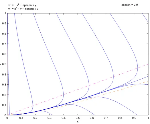
A computer-generated phase portrait for the planar reduction (3), restricted to the physically relevant and positively invariant nonnegative quadrantS, is given in Figure 1. In this paper, we will develop precise mathematical properties of the phase portrait. Equivalently, we develop results on solutions of the scalar reduction (5).
The horizontal and vertical isoclines for the planar system (3), which are found by re-spectively setting ˙y= 0 and ˙x= 0, are given by
y=H(x) := x 2
1 +εx and y =V(x) := x
ε. (7)
x ’ = − x2 + epsilon x y
y ’ = x2 − y − epsilon x y
epsilon = 2.0
0 0.1 0.2 0.3 0.4 0.5 0.6 0.7 0.8 0.9 1 0
0.1 0.2 0.3 0.4 0.5 0.6 0.7 0.8 0.9 1
x
y
Figure 1: A phase portrait for (3) for parameter value ε= 2.0 along with the isoclines.
H(0) = 0 =V(0), both H and V are strictly increasing, and V(x)> H(x) for all x >0. It appears from the phase portrait that the region between the isoclines,
Γ0 :={(x, y) : x >0, H(x)≤ y≤V(x)},
acts like a trapping region for (time-dependent) solutions of the planar reduction. Moreover, the origin appears to be globally asymptotically stable.
Theorem 2. Consider the planar system (3).
(a) The region Γ0 is positively invariant.
(b) Let x(t) be the solution with initial condition x(0) =x0, where x0 ∈ {x∈S : x >0}.
Then, there is a t∗
≥0 such that x(t)∈Γ0 for all t≥t∗.
(c) Let x(t) be the solution with x(0) =x0, where x0 ∈S. Then, x(t)→0 as t→ ∞.
Proof:
(a) It follows from the definition (4) of the vector field g that g•ν <0 along V and H,
(b) We will break the proof into cases.
Case 1: (x0, y0)∈Γ0. Since Γ0 is positively invariant, x(t)∈Γ0 for all t≥0.
Case 2: x0 >0 and y0 > V(x0). Suppose, on the contrary, thatx(t) does not enter Γ0. It follows that y(t)> V(x(t)) for all t≥0. Using the differential equation (3), we know ˙x(t)>0 and ˙y(t)<0 for allt ≥0. Now, we see from the definition (6) of the function f that
˙
y(t) ˙
x(t) =f(x(t), y(t)) =−1−
y(t)
εx(t)y(t)−x(t)2 <−1 for all t≥0.
Note thatεxy−x2 >0 since y > V(x) =x/ε and x, y >0. Thus,
˙
y(s)<−x˙(s) for all s≥0.
Integrating with respect to s from 0 to t and rearranging, we obtain
y(t)≤y0−[x(t)−x0] for all t≥0.
Let (x1, V(x1)) be the point of intersection of the vertical isocline y=V(x) and the straight line y =y0−(x−x0). Obviously, x1 > x0. Since x(t) is monotone increasing and bounded above byx1, we see that there is anxb∈[x0, x1] such that
x(t)→bxast→ ∞. Similarly, sincey(t) is monotone decreasing and bounded below byV(x0), we see that there is ayb∈[V(x0), y0] such thaty(t)→ybast→ ∞. Thus, the ω-limit set is ω(x0, y0) = {(bx,by)}. Since ω(x0, y0) is invariant and (0,0) is the only equilibrium point of the system, bx= 0 andyb= 0. This is a contradiction.
Case 3: x0 >0 and 0≤y0 < H(x0). This case is proved in a manner similar to Case 2.
(c) If x0 = 0, the solution of (3) is x(t) = (0, y0e
−t
)T. This clearly satisfies x(t)→0 as
t→ ∞. Thus, we can assume x0 >0 and, by virtue of part (b), we can assume further that (x0, y0)∈Γ0. It follows from the differential equation (3) and the fact that Γ0 is positively invariant that ˙x(t)≤0 and ˙y(t)≤0 for allt≥0. Since both x(t) andy(t) are decreasing and bounded below by zero, by the Monotone Convergence Theorem we know that there are xb and ybsuch that x(t)→bx and y(t)→ybas t→ ∞. Thus, the ω-limit set is ω(x0, y0) ={(x,b yb)}. Since ω(x0, y0) is invariant and (0,0) is the only equilibrium point of the system, xb= 0 and by= 0.
are strictly decreasing. In terms of the Lindemann mechanism (1), Theorem 2 tells us that after sufficient time the concentrations of A and B will be strictly decreasing. Moreover, experimentally it is an easy matter to determine in which of these three regions a planar solution lies.
Remark 4. We have shown that the origin for the planar system (3) is globally asymptoti-cally stable (with respect to the nonnegative quadrant) for all values of the parameterε >0. In terms of the Lindemann mechanism (1), this means that A (and B) will be completely converted (as time tends to infinity) into the product P for all initial conditions and values of the rate constants.
The Jacobian matrix at the origin for the planar system (3) is diag (0,−1). Thus, the origin is a nonhyperbolic fixed point. The Hartman-Grobman Theorem, unfortunately, can-not be applied here. Using Theorem 65 in §9.21 of [1], the origin is a saddle node which consists of two hyperbolic sectors and one parabolic sector. As we will effectively show later,
S is contained in the parabolic sector.
3
The Isocline Structure
The horizontal and vertical isoclines, along with all isoclines between them, will be very useful. If we solve f(x, y) = cfor y, we obtain y=F(x, c), where
F(x, c) := x 2
K(c) +εx, c=6 −1, x6=−ε −1
K(c), (8)
and
K(c) := 1
1 +c, c6=−1. (9)
That is, y =F(x, c) is the isocline for slope c. Note that K(c) is a hyperbola with vertical asymptote atc=−1. Note also that each isocline, forc∈R\ {−1}, has a vertical asymptote atx=−ε−1
K(c).
Remark 5. The interior of the region Γ0 corresponds to 0< c <∞ and 0< K(c)<1.
Remark 6. Two exceptional isoclines arey =V(x) (the vertical isocline) and y= 0 which correspond, respectively, to
lim
c→∞F(x, c) = x
ε and clim→−1F(x, c) = 0.
Claim 7. Let c∈R\ {−1} and let w(x) := F(x, c) be the isocline for slope c. Then, the derivative of w satisfies
lim
x→∞w ′
(x) =ε−1
. (10)
Furthermore, w is concave up for all x >−ε−1
K(c) and satisfies the differential equation
x2w′
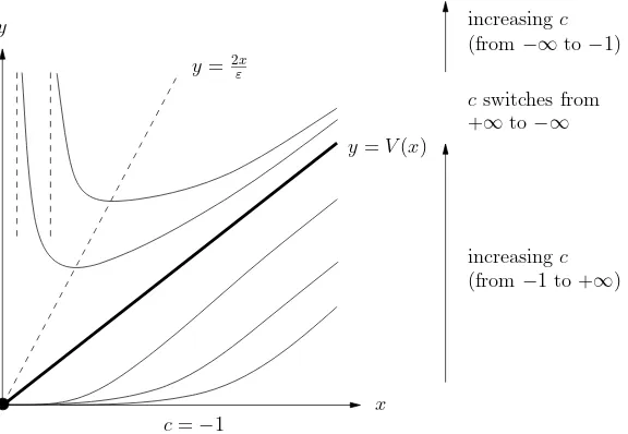
increasingc (from−1 to +∞)
increasingc (from−∞to−1)
cswitches from +∞to−∞
x c=−1
y
y=2x ε
y=V(x)
Figure 2: Sketch of the isocline structure of (5). The isoclines above the vertical isocline have zero slope along the liney = 2x/ε.
Proof: The proof is straight-forward and omitted.
Remark 8. The vertical isocline satisfies the limit (10) and the differential equation (11). The isocline w(x) = 0 (the isocline for slope −1) also satisfies the differential equation but does not satisfy the limit.
The isocline structure is sketched in Figure 2. We will often appeal to the isocline structure. For example, if a scalar solution of (5) is above the line y= 0 and below the horizontal isocline y=H(x), we know that−1< y′
(x)<0.
4
Existence and Uniqueness of the Slow Manifold
It appears from the given phase portrait, Figure 1, that there exists a unique solution to (5) that lies entirely in the region between the horizontal and vertical isoclines. To prove this, we will need to use a nonstandard version of the Antifunnel Theorem. See, for example, Chapters 1 and 4 of [13].
Definition 9. Let I = [a, b) or I = (a, b) be an interval (where a < b≤ ∞) and consider the first-order differential equation y′
=f(x, y) over I. Let α, β ∈C1(I,R) be functions satisfying
α′
(x)≤f(x, α(x)) and f(x, β(x))≤β′
(a) The curves α and β satisfying (12) are, respectively, a lower fence and an upper fence. If there is always a strict inequality in (12), the fences are strong. Otherwise, the fences are weak.
(b) If β(x)< α(x) on I, then the set Γ is called an antifunnel, where
Γ :={(x, y) : x∈I, β(x)≤y≤α(x)}.
Theorem 10 (Antifunnel Theorem, p.196 of [13]). Let Γ be an antifunnel with strong lower and upper fences α and β, respectively, for the differential equation y′
=f(x, y) over the interval I, where I = [a,∞) or I = (a,∞). Suppose that there is a function r such that
r(x)< ∂f
∂y(x, y) for all (x, y)∈Γ and xlim→∞
α(x)−β(x)
exp Rax r(s)ds = 0.
Then, there exists a unique solution y(x) to the differential equation y′
=f(x, y) which sat-isfies β(x)< y(x)< α(x) for all x∈I.
Remark 11. The standard version of the Antifunnel Theorem applies to antifunnels that are narrowing. That is, where α(x)−β(x)→0 as x→ ∞. This version applies to, for example, the Michaelis-Menten mechanism [4].
4.1
Existence-Uniqueness Theorem
We want to show that there is a unique scalar solution that lies entirely in the region Γ0. However, the vertical isocline is not a strong lower fence since “f(x, V(x)) = ∞.” This turns out to be a fortunate obstacle.
Suppose that we want the isocline
w(x) := x 2
r+εx, 0< r <1
to be a strong lower fence for the differential equation (5) for all x >0. Note that the condition on r restricts the isocline to being between the horizontal and vertical isoclines. Note also that
f(x, w(x)) = K−1
(r) for all x >0.
Since w is concave up and satisfies the limit (10), we know that w′
(x)< ε−1
for all x >0. Hence,
ε−1
≤K−1
(r) =⇒ w′
(x)< f(x, w(x)) for all x >0.
Since we want the isocline that will give us the thinnest antifunnel, we choose
α(x) := x 2
K(ε−1
Note thatα(x) is the isocline for slope ε−1
and
K ε−1
= ε
1 +ε.
Hence, define the region
Γ1 :={(x, y) : x >0, H(x)≤y≤α(x)}.
We will show that Γ1 indeed has a unique scalar solution. First, we need a claim.
Claim 12.
(a) Suppose that x >0 and H(x)≤y < V(x). Then,
∂f
∂y(x, y)> ε
2,
where f is as in (6).
(b) Let y1(x) and y2(x) be two scalar solutions to (5) satisfying
H(x)≤y1(x)≤y2(x)< V(x) for all x∈[a, b],
where 0< a < b. If we define u(x) := y2(x)−y1(x), then
u(x)≥u(a)eε2(x−a)
for all x∈[a, b].
Proof:
(a) Using (7),
εx2
1 +εx ≤εy < x and 0< x−εy≤x− εx2 1 +εx.
Rearranging, we have
0< 1 +εx x ≤
1
x−εy and 0<
1
x +ε
2
≤ 1
(x−εy)2.
Thus, using the definition (6) of f we have
∂f
∂y(x, y) =
1
(x−εy)2 ≥
1
x +ε
2
(b) We will use an adaptation of the method used to prove uniqueness in the Antifunnel Theorem. By the Fundamental Theorem of Calculus,
u′
(x) =
Z y2(x)
y1(x)
∂f
∂y(x, y)dy for all x∈[a, b],
where f is given in (6). Since∂f(x, y)/∂y > ε2 for allx∈[a, b], for all s∈[a, b] we have
u′(s)≥ε2u(s) =⇒ d
ds
e−ε2(s−a)u(s)≥0.
If we integrate with respect to s from a to x and then solve for u(x), we obtain the conclusion.
Theorem 13.
(a) There exists a unique solution y =M(x) (the slow manifold) contained in Γ1 for the
scalar differential equation (5).
(b) The solution y =M(x) is also the only solution that lies entirely in Γ0.
Proof:
(a) We have already established that α is a strong lower fence. To show that H is a strong upper fence, observe
f(x, H(x)) = 0< H′
(x) for all x >0.
Moreover, α(x)> H(x) for all x >0. By definition, Γ1 is an antifunnel. We know from Claim 12 that ∂f(x, y)/∂y > ε2 inside Γ
1. Hence, we can apply the Antifunnel Theorem with r(x) :=ε2. To see why, observe that
Z ∞
0
r(x)dx=∞, lim
x→∞[α(x)−H(x)] =
1
ε2(1 +ε), and xlim→∞
α(x)−H(x)
exp R0x r(s)ds = 0.
Therefore, there is a unique solution y=M(x) to (5) that lies in Γ1 for all x >0.
(b) Using (7), it is quickly verified that
V(x)−H(x) = 1
ε2 +O
1
x
as x→ ∞.
Since Γ1is contained in Γ0, we know thatM(x) is contained in Γ0 for allx >0. Suppose, on the contrary, that there is a second solution y(x) contained in Γ0 for all x >0. We know, by virtue of Claim 12, thatu(x) :=|y(x)− M(x)| satisfiesu(x)→ ∞asx→ ∞. This is impossible.
Remark 14. We are referring to the unique solution between the horizontal and vertical isoclines as the slow manifold. However, all scalar solutions in Γ0 are technically slow man-ifolds (and, as it turns out, centre manman-ifolds). This is because, as functions of time, the solutions approach the origin in the slow direction.
Remark 15. There is no isocline w(x) such that w(x)> H(x) and w(x) is a strong upper fence for allx >0. To see why this is the case, supposew(x) :=F(x, c), wherec >0, satisfies
w′
(x)> f(x, w(x)) for all x >0. This is impossible, since f(x, w(x)) =c for all x >0 and
w′
(x)→0 as x→0+.
Proposition 16. Letybe a solution to (5) lying insideΓ1 forx∈(0, a), wherea >0. Then,
we can extend y(x) and y′
(x) to say y(0) = 0 and y′
(0) = 0.
Proof: Observe that
lim
x→0+α(x) = 0 and xlim→0+
α(x)
x = 0.
Since
0< y(x)< α(x) for all x∈(0, a),
the Squeeze Theorem establishes y(0) = 0. Now,
0< y(x)−y(0) x−0 <
α(x)
x for all x∈(0, a).
Thus, y′
(0) = 0 by the Squeeze Theorem again and the definition of (right) derivative.
4.2
Nested Antifunnels
The region Γ1 is the thinnest antifunnel for x >0 with isoclines as boundaries. However, we can find thinner antifunnels than Γ1 which are valid for different intervals. For an iso-cline w(x) :=F(x, c), where 0< c < ε−1
, to be a strong lower fence on an interval, we need
w′
(x)< f(x, w(x)). Solving the equationw′
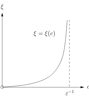
(x) = f(x, w(x)), as we shall see, givesx=ξ(c), where
ξ(c) :=
K(c)
ε
1
√
1−εc −1
, c∈ 0, ε−1
. (14)
ξ
c ε−1
ξ = ξ(c)
Figure 3: Graph of the functionξ(c) for arbitraryε >0.
Claim 17.
(a) The function ξ(c) satisfies
lim
c→0+ξ(c) = 0, lim
c→(ε−1)−
ξ(c) =∞, and ξ′
(c)>0 for all c∈ 0, ε−1
. (15)
(b) The function ξ(c) is analytic for all c∈(0, ε−1
). Furthermore, ξ(c)has analytic inverse ξ−1
(x) defined for all x >0.
Proof: The proof is routine, tedious, and omitted.
Proposition 18. Let c∈(0, ε−1
) and w(x) :=F(x, c).
(a) The isocline w satisfies
w′
(x)
< f(x, w(x)), if 0< x < ξ(c) =f(x, w(x)), if x=ξ(c)
> f(x, w(x)), if x > ξ(c)
.
(b) The slow manifold satisfies
Proof:
(a) Note that f(x, w(x)) =c for all x >0. If we set w′
(x) =c, we obtain
ε(1−εc)x2+ 2K(c) (1−εc)x−cK(c)2 = 0.
This has two roots, one negative and one positive. The positive root is given byx=ξ(c) with ξ(c) as in (14). It is a routine matter to confirm that w′
(x)< f(x, w(x)) when 0< x < ξ(c) and that w′
(x)> f(x, w(x)) when x > ξ(c).
(b) It follows from the Antifunnel Theorem.
5
Concavity
In this section, we will establish the concavity of all scalar solutions, except for the slow manifold, in the nonnegative quadrant. The concavity of the slow manifold will be established later. These results will be obtained by using an auxiliary function. Moreover, we will construct a curve of inflection points which approximates the slow manifold.
5.1
Establishing Concavity
Let y be a solution to (5) and consider the function f given in (6). If we differentiate
y′
(x) =f(x, y(x)) and apply the Chain Rule, we obtain
y′′
(x) =p(x, y(x))h(x, y(x)), (16)
where
p(x, y) := 1
x2(εy−x)2 and h(x, y) :=x
2f(x, y) +y(εy
−2x). (17)
The functionp(x, y) is positive everywhere except along the vertical isocline and forx= 0, where it is undefined. We will be considering the functions h(x, y) andp(x, y) along a given solutiony(x) so we will abuse notation by writing h(x) :=h(x, y(x)) andp(x) :=p(x, y(x)). For a given x >0 with y(x)6=V(x), it follows from (16) and the fact thatp(x)>0 that the sign of h(x) is the same as the sign of y′′
(x). Furthermore, if we differentiate h(x) with respect to xand apply (16), we see that the function h has derivative
h′
(x) =x2p(x)h(x) + 2y(x) [εy′
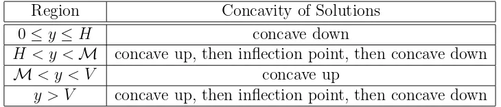
Region Concavity of Solutions
0≤y≤H concave down
H < y < M concave up, then inflection point, then concave down
M< y < V concave up
y > V concave up, then inflection point, then concave down
Table 1: A summary of the concavity of solutions of (5) in the nonnegative quadrant.
Claim 19. Let y be a solution to (5) and let x0 >0 with y(x0)6=V(x0). Consider the
isocline through the point (x0, y(x0)), which is given by w(x) :=F(x, y′(x0)). Then,
h(x0) =x0[y
′
(x0)−w
′
(x0)].
Furthermore,
y′′
(x0)>0⇐⇒y
′
(x0)> w
′
(x0) and y
′′
(x0)<0⇐⇒y
′
(x0)< w
′
(x0).
Proof: The first part follows from (11) and (17). The second part follows from the first.
The concavity of all solutions in all regions of the nonnegative quadrant (but not at the origin) can be deduced using the auxiliary function h, properties of scalar solutions we have already developed, elementary results like Rolle’s Theorem and the Intermediate Value Theorem, and the following easy-to-verify lemma. Table 1 summarizes the results we will state more precisely in this section.
Lemma 20. LetI be one of the intervals[a, b], (a, b),[a, b), and(a, b]. Suppose thatφ∈C(I)
is a function having at least one zero in I.
(a) If I = (a, b] or I = [a, b], then the function φ has a right-most zero in I. Likewise, if I = [a, b) or I = [a, b], then the function φ has a left-most zero inI.
(b) If φ∈C1(I) and φ′
(x)>0 for every zero of φ in I, then φ has exactly one zero in I.
Proposition 21. Letybe a solution to (5)lying belowH with domain[a, b], where0< a < b, y(a) = H(a), and y(b) = 0. Then, y is concave down on [a, b].
Proposition 22. Let y be a solution to (5)lying above H and below M with domain (0, a], where a >0 and y(a) = H(a). Then, there is a unique x1 ∈(0, a) such that y′′(x1) = 0.
Moreover, y is concave up on (0, x1) and concave down on (x1, a].
Proof: Leth be as in (17) defined with respect to the solution y. Now, we know y′
(a) = 0 and, by Proposition 16, we can extendy′
(x) continuously and writey′
(0) = 0. By Rolle’s The-orem, there is an x1 ∈(0, a) such that y
′′
(x1) = 0 and henceh(x1) = 0. To show the unique-ness ofx1, suppose thatx2 ∈(0, a) is such thath(x2) = 0. Now, sinceH(x2)< y(x2)< α(x2), by virtue of the isocline structure 0< y′
(x2)< ε
−1
. Moreover, we can see from (18) that
h′
(x2)<0. By Lemma 20, we can conclude x2 =x1. Finally, by continuity we can conclude that h(x)>0 on (0, x1) and h(x)<0 on (x1, a] since h(a) =y(a) [εy(a)−2a]<0.
Proposition 23. Let y be a solution to (5) strictly between M and V with domain (0, a), where a >0 and y(a−) =V(a). Then, y is concave up on (0, a).
Proof: Omitted in the interest of space.
Proposition 24. Let y be a solution to (5) lying above V with domain (0, a), where a >0, y(0+) =∞, and y(a−) =V(a). Then, there is a unique x1 ∈(0, a) such that y′′(x1) = 0.
Moreover, y is concave up on (0, x1) and concave down on (x1, a).
Proof: Omitted in the interest of space.
5.2
Curve of Inflection Points
We know from Table 1 that solutions to the scalar differential equation (5) can only have inflection points between H and M or above V. We can construct a curve of inflection points, between H and M, which is close to the slow manifold.
It is easily verified that
h(x, y) = ε
2y3−(3εx)y2+ (2x2−εx2 −x)y+x3
εy−x ,
where h is as in (17). Thus, there are three curves along which solutions have zero second derivative, given implicitly by
ε2y3−(3εx)y2+ 2x2−εx2−xy+x3 = 0.
x
1 0.8 0.6 0.4 0.2 0
y 2
1.5
1
0.5
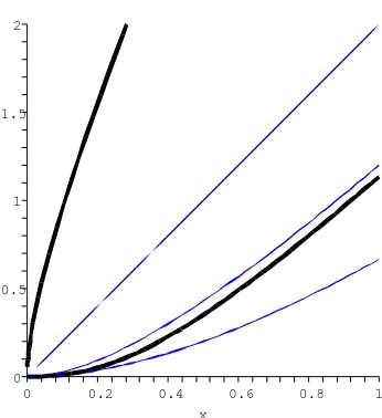
0
Figure 4: The two thick curves are curves along which solutions of (5) have inflection points, for parameter valueε= 0.5. The thin curves are the horizontal, α, and vertical isoclines. We will show later that the slow manifold lies between the lower thick curve and the middle thin curve.
Recall that, for a fixed c∈(0, ε−1
), the isocline w(x) :=F(x, c) switches from being a strong lower fence to being a strong upper fence at x=ξ(c) and y=F(ξ(c), c), where F is defined in (8) andξ is defined in (14). As it turns out,
Y(x) :=F x, ξ−1
(x), x >0 (19)
will be a curve of inflection points between H and M. Note that H(x)< F(x, c)< α(x) for all x >0 and c∈(0, ε−1
), which follows from the isocline structure. Moreover, note 0< ξ−1
(x)< ε−1
for all x >0. Thus, H(x)<Y(x)< α(x) for all x >0.
Claim 25. Suppose that x0 >0andH(x0)< y0 < α(x0). Define the slope c:=f(x0, y0)and
isocline w(x) :=F(x, c). Then, the isocline w satisfies
w′
(x0)
> f(x0, y0), if H(x0)< y0 <Y(x0) =f(x0, y0), if y0 =Y(x0)
< f(x0, y0), if Y(x0)< y0 < α(x0)
.
Proof: Note that 0< c < ε−1
and y0 =w(x0). We will only show the third case since the other two cases are similar. Assume that Y(x0)< y0 < α(x0). Appealing to the iso-cline structure, we know ∂f(x, y)/∂y >0 if x >0 and H(x)< y < α(x). Consequently,
f(x0, y0)> f(x0,Y(x0)). Since c=f(x0, y0) and ξ−1(x0) =f(x0,Y(x0)), we can conclude
c > ξ−1
(x0). Since ξ is strictly increasing, x0 < ξ(c). By virtue of Proposition 18, we can conclude w′
Claim 26. The curve y=Y(x) is analytic for all x >0.
Proof: We know thatξ−1
(x) is analytic and 0< ξ−1
(x)< ε−1
for allx >0. Since F(x, c) is analytic if x >0 and 0< c < ε−1
, we see from the definition (19) that Y(x) is analytic for
allx >0.
Proposition 27. The function h, defined in (17), satisfies
h(x, y)
<0, if x >0, H(x)< y <Y(x) = 0, if x >0, y=Y(x)
>0, if x >0, Y(x)< y < α(x)
.
Proof: Let x0 >0 and H(x0)< y0 < α(x0) be fixed. Consider the slope c:=f(x0, y0) and isocline w(x) :=F(x, c). We know from Claim 19 that
h(x0, y0) =x0[f(x0, y0)−w
′
(x0)].
The result follows from Claim 25.
Proposition 28. The curve y =Y(x) satisfies
H(x)<Y(x)<M(x) for all x >0.
Proof: We know already thatH(x)<Y(x)< α(x) for allx >0. We know from our results on concavity (see Table 1) that h(x, y)>0 if x >0 and M(x)< y < α(x), where h is the function defined in (17). By continuity, we can conclude h(x,M(x))≥0 for all x >0. It follows from Proposition 27 that Y(x)≤ M(x) for all x >0.
To establish a strict inequality, let h be defined along the solution y=M(x). Assume, on the contrary, that there is an x0 >0 such that h(x0) = 0. Using (18), h
′
(x0)<0. This
contradicts the fact that h(x)≥0 for all x >0.
5.3
Slow Tangent Manifold
linearization matrixA(x) :={gij(x)}2i,j=1, where gij(x) :=∂gi(x)/∂xj, which has character-istic equation
λ2−τ λ+ ∆ = 0, where τ :=g11+g22 and ∆ :=g11g22−g12g21.
For notational brevity, we are suppressing the dependence on x.
Claim 29. Suppose 4∆ < τ2 and g
126= 0. Then, A has real distinct eigenvalues and
asso-ciated distinct eigenvectors given, respectively, by
λ±:=
τ±√τ2−4∆
2 and v± :=
1
σ±
, where σ± :=
λ±−g11 g12
.
Proof: The proof is routine.
Proposition 30. Suppose that g1 6= 0, g12= 06 , and 4∆< τ2 at some fixed point (a, b) and
let y(x)be the scalar solution through (a, b). Then, y′′
(a) = 0 if and only ifg k v+ or g k v− at (a, b).
Proof: First, note that σ± is the slope of the eigenvector v±. If we differentiate the scalar
differential equation and manipulate the resulting expression, we obtain
y′′ = −g12[(g2/g1)−σ+] [(g2/g1)−σ−]
g1
.
The conclusion follows.
For the specific planar and scalar systems (3) and (5), we have
A=
−2x+εy εx
2x−εy −εx−1
, τ =−(ε+ 2)x+εy−1, and ∆ = 2x−εy.
To apply Proposition 30, we need to verify that g1 6= 0, ∂g1/∂y 6= 0, and τ2 >4∆ in the relevant regions. Trivially, g1 6= 0 (except along the vertical isocline) and g12>0 for x >0. To show thatτ2 >4∆ for x >0, observe
τ2−4∆ =ε2
y− (ε+ 2)x−1 ε
2
+ 4εx ≥4εx >0.
This establishes that Y is a tangent manifold. To establish that Y is indeed a slow tangent manifold, we note that (as can be shown) λ− < λ+ <0, σ− <0< σ+, and g2/g1 >0 for
every x∈Γ1. We have thus demonstrated the following.
6
Behaviour of Solutions Near the Origin
In this section, we establish the full asymptotic behaviour of scalar solutionsy(x) asx→0+. Moreover, we will obtain the leading-order behaviour of planar solutions x(t) as t→ ∞.
6.1
Scalar Solutions
We will begin by attempting to find a Taylor series solution. Consider the differential equa-tion (5), which can be rewritten
εxyy′
−x2y′
−x2 +y+εxy= 0. (20)
Assume that y(x) is a solution in Γ0 of the form
y(x) =
∞
X
n=0
bnxn (21)
for undetermined coefficients {bn}
∞
n=0. If we substitute the series (21) into (20) and then solve for the coefficients, we obtain
b0 = 0, b1 = 0, b2 = 1, b3 = 2−ε,
and bn= (n−1−ε)bn−1−ε
n−2
X
m=2
(n−m)bmbn−m for n≥4. (22)
We will use centre manifold theory to show that the series (21) is fully correct for each solution inside the trapping region Γ0. However, we must first show that each solution is a centre manifold. That is, we must show that each solution y(x) satisfies y(0) = 0 and
y′
(0) = 0. Proposition 16 already established that this is true for y(x) inside Γ1.
Proposition 32. Letybe a solution to (5) lying insideΓ0 forx∈(0, a), wherea >0. Then,
we can extend y(x) and y′
(x) to say y(0) = 0 and y′
(0) = 0.
Proof: These limits have already been established if yis the slow manifold or ifylies below the slow manifoldM. Hence, we will assume that
M(x)< y(x)< V(x) for all x∈(0, a).
Let c:=y′
(a/2). We know from Table 1 that y is concave up on (0, a/2). Since M(x)>0 for x∈(0, a/2), we thus have
where F is the function given in (8). Note that
lim
x→0+F(x, c) = 0 and xlim→0+
F(x, c)
x = 0.
It follows from the Squeeze Theorem that we can takey(0) = 0. Now, observe that
0< y(x)−y(0) x−0 <
F(x, c)
x .
Again by the Squeeze Theorem, we see that we can take y′
(0) = 0.
Theorem 33. Lety(x)be a scalar solution to (5)lying insideΓ0 and consider the coefficients
{bn}
Proof: The Centre Manifold Theorem guarantees that there is a solution u(x) to (5) such that
n=2 since they are gen-erated uniquely by the differential equation. Since y(x) is a centre manifold, it follows from centre manifold theory that
y(x)−u(x) =O xk as x→0+
for anyk ∈ {2,3, . . .}. See, for example, Theorem 1 on page 16, Theorem 3 on page 25, and properties (1) and (2) on page 28 of [5]. The conclusion of the theorem follows.
Remark 34. For analytic systems of ordinary differential equations for which the Centre Manifold Theorem applies, if the Taylor series for a centre manifold has a nonzero radius of convergence, then the centre manifold is unique. Since all solutions y to (5) lying inside Γ0 are centre manifolds, we can conclude that the Taylor series
P∞
n=2bnxn has radius of convergence zero.
Remark 35. We know from Theorem 2 that any planar solutionx(t) withx0 >0 eventually enters the region Γ0 and approaches the origin as t→ ∞. Now, it follows from Theorem 33 that, ast → ∞, the corresponding scalar solution satisfies
y(x) =x2+O x3 as x→0+.
If we revert to the original dimensional quantities for the Lindemann mechanism (1), this means
6.2
Planar Solutions
We can use the isoclines to extract the leading-order behaviour of planar solutions as time tends to infinity.
Proof: Letc >0 be fixed and arbitrary. We know from Theorem 2, Table 1, and the isocline structure that there exists a T ≥0 such that
H(x(t))≤y(t)≤F(x(t), c) for all t≥T, (23)
whereb :=ε/K(c) andK is the function defined in (9). Note that the solution of the initial value problem
where W is the Lambert W function [6]. A simple comparison argument applied to (24) establishes
ϕ(t;ε, T, x(T))≤x(t)≤ϕ(t;b, T, x(T)) for all t≥T. (25)
A standard property of the Lambert W function is
W(t) = ln(t)−ln(ln(t)) + o(ln(ln(t))) as t→ ∞.
Consequently, it can be shown
W et=t
With a little manipulation, it can be verified that
for any a, u0 >0 and t0 ≥0. It follows from (25) that
This yields the desired conclusion forx(t). The conclusion fory(t) follows from the conclusion
for x(t) and Theorem 33.
Remark 37. The horizontal isocline, explicitly given in (7), satisfies
H(x)≡ x 2
1 +εx =x
2
−εx3+O x4 as x→0+.
It follows from the differential equation (3) for y(t), Theorem 33, and Proposition 36 that, for any planar solution with x0 >0,
˙
Phrasing this in terms of the original dimensional quantitiesa(τ) andb(τ) for the Lindemann mechanism (1),
That is, provided the decaying molecule A is initially present (a0 >0), the QSSA is valid after sufficiently much time for all values of the rate constants and initial concentrations.
It is possible to derive the expression forx(t) in Proposition 36 without appealing to the isocline structure and concavity. To achieve this, we will note thatx(t) satisfies the integral equation and then twice utilize the following easy-to-verify lemma.
We know from Theorems 2 and 33 that
x(t) = o(1), y(t) = o(1), and y(t)
x(t)+ 1 = 1 + o(1) as t→ ∞. It follows from Lemma 38 that
Z t By virtue of the integral equation (26),
1
(Note that the constant term−1/x0 in the integral equation is absorbed into the error term o(t).) To take this one step further, observe now that
y(t)
which follows from Theorem 33, and so by Lemma 38 we have
Z t
Remark 39. Using Theorem 33 and Proposition 36, we have the updated estimate
y(t)
It follows from the Fundamental Theorem of Calculus and the estimate (27) that, for any
a >0, Rat u′
(s)ds=ra+ o(1) as t→ ∞ for some constant ra. Again by the Fundamen-tal Theorem of Calculus, u(t) =c+ o(1) as t → ∞, where c:=ra+u(a). (Note that the constant ccannot depend on the choice of a.) Thus,
Z t
0
y(s)
x(s)ds= ln(t) +c+ o(1) as t→ ∞.
Consequently, the error terms in Proposition 36 for x(t) and y(t), respectively, can be im-proved to be, in terms of c,
7
All Solutions Must Enter the Antifunnel
Earlier, in Theorem 2, we showed that all solutionsx(t) to the planar system (3), except for the trivial solutions, eventually enter the trapping region Γ0. Here, we show that Γ1 is itself a trapping region.
Theorem 40. Let x(t) be the solution to (3)with x(0) =x0, where x0 ∈ {x∈S : x >0}.
(a) There is a t∗
≥0 such that x(t)∈Γ1 for all t ≥t∗.
(b) Define the region
Γ2 :={(x, y) : x >0, Y(x)≤ y≤α(x)}.
Then, there is a t∗
≥0 such that x(t)∈Γ2 for all t≥t
∗ .
Proof:
(a) We know from Theorem 2 that x(t) eventually enters and stays in Γ0. Let y(x) be the corresponding scalar solution to (5). Then, we can say y′
(0) = 0. Appealing to the isocline structure, this means that x(t) has entered Γ1. Furthermore, since g•ν <0
along the horizontal andα isoclines which form the boundaries of the region in question, we see that Γ1 is positively invariant.
(b) It follows from Table 1, Proposition 27, and the previous part of the theorem.
8
Properties of the Slow Manifold
In this section, we will highlight some properties of the slow manifold.
Proposition 41. The slow manifold y=M(x)satisfies
0< H(x)<Y(x)<M(x)< α(x) for all x >0 and lim
x→0+M(x) = 0.
Proof: The first part follows from Theorem 13 and Proposition 28. The second part follows
from the Squeeze Theorem.
Proof: It follows from Propositions 27 and 41 thath(x,M(x))>0 for all x >0, where his the function defined in (17). Since sgn(M′′
(x)) = sgn(h(x,M(x))), it must be that the slow
manifold is concave up for all x >0.
Proposition 43. The slope of the slow manifold y=M(x) satisfies
0<M′
(x)< ε−1
for all x >0, lim
x→0+M
′
(x) = 0, and lim
x→∞M
′
(x) =ε−1 .
Proof: The first part is a consequence of Proposition 41 and the isocline structure. The first limit is a special case of Proposition 32. To prove the second limit, let c∈(0, ε−1
). It follows from Proposition 18 and the isocline structure that
c <M′
(x)< ε−1
for all x > ξ(c),
where ξ is the function defined in (14). Applying (15) and the Squeeze Theorem gives the
second limit.
Remark 44. The justification which Fraser provides in [9] (just before Theorem 1) that
M′
(x)→ε−1
asx→ ∞ is incorrect. The error is that the distance between the horizontal and vertical isoclines does not tend to zero as x tends to infinity. Thus, the asymptotic behaviour of M′
(x) need not be the same as the asymptotic behaviour of H′
(x) and V′
(x).
Proposition 45. Asymptotically, the slow manifold can be written
M(x)∼
∞
X
n=2
bnxn as x→0+,
where the coefficients {bn}
∞
n=2 are as in (22).
Proof: Since the slow manifold is contained entirely in Γ0, we can apply Theorem 33.
Corollary 46. The slow manifold satisfies
M(x) =H(x) +O x3 as x→0+.
Moreover, this statement would not be true if we replaceH(x)with any other isoclineF(x, c).
Proof: It follows from a comparison of the asymptotic expansions for M(x), H(x), and
F(x, c).
to find a series in integer powers of x. Third, we will prove definitively that the resulting series is indeed fully correct.
Let c∈(0, ε−1
). We know from Proposition 18 that
F(x, c)<M(x)< α(x) for all x > ξ(c),
Assume that we can write
M(x) =
for undetermined coefficients {ρn}
∞
n=−1. Based on the above analysis using isoclines, we
expect ρ−1 =ε −1
and ρ0 =−ε−1(1 +ε)
−1
. If we substitute (28) into (20) and solve for the coefficients, we obtain
Proposition 47. Asymptotically, the slow manifold can be written
M(x)∼
where the coefficients {ρn}
∞
Proof: To prove the result, we will apply the Centre Manifold Theorem to a fixed point at infinity. Consider the change of variables
X :=x−1
and Y :=y−r(x), where r(x) :=ρ−1x+ρ0+ρ1x −1
,
with the coefficients ρ−1,ρ0, andρ1 being given in (29). If we differentiate the new variables
with respect to time and use the differential equation (3), we obtain a planar differential equation ˙X =G(X), where X:= (X, Y)T. Now, the system ˙X=G(X) is not polynomial. However, the system ˙X=Gb(X), whereGbi :=XGi(fori= 1,2), is polynomial. Importantly, the two systems ˙X=G(X) and ˙X =Gb(X) both have the same scalar reduction. Now, the system ˙X=Gb(X) is in the canonical form for the Centre Manifold Theorem with lineariza-tion matrix diag (0,−1−ε). By the Centre Manifold Theorem, there is aC∞
centre manifold at the origin (X, Y) = (0,0). It can be shown that the origin is a saddle node (a degenerate saddle) with the physically relevant portion of the phase portrait X ≥0 consisting of two hyperbolic sectors and a unique solution (the centre manifold) approaching the origin. We know from our analysis that this unique solution is indeed the slow manifold.
Since the centre manifold isC∞
, the slow manifold can be writtenM(X)∼P∞n=2ρbnXn as X →0+ in the new coordinates for some coefficients {ρb
n}
∞
n=2. Upon reverting back to original coordinates and observing that the coefficients in (29) are generated uniquely from
the differential equation, the conclusion follows.
Corollary 48. The slow manifold satisfies
M(x) =α(x) +O
Proof: It follows from a comparison of the asymptotic expansions for M(x), α(x), and
F(x, c).
Remark 49. Consider any isocline y=F(x, c), where c≥0 and F(x, c) is the function defined in (8) which satisfies
F(x, c) =
Observe that the leading-order behaviour is the same for any slope cbut the following term (the constant term) distinguishes each isocline. In terms of the dimensional variables for the Lindemann mechanism (1), the leading-order behaviour is (k1/k−1)a. This is the same as
one obtains by applying the QSSA for the so-called high-pressure regime. However, as we know from the phase portrait and Corollary 48, planar solutions approach the slow manifold with α(x) being the best isocline approximation to M(x) for largex. Moreover, observe
This explains why the QSSA has been known to be unreliable in the high-pressure regime when k1 is large (or, equivalently, when ε is small).
9
Open Questions
It would be nice to extend Proposition 36 to include more terms. In particular, it is desirable to have the lowest-order term which depends on the initial condition. Forx(t), it is expected that the initial condition x0 first appears in the 1/t2 term since this is the case whenε = 0, which has
x(t) = x0 1 +x0t ∼
∞
X
n=1
(−1)n+1
xn−1
0 tn
as t→ ∞.
More generally, we would like to develop an iterative procedure to extract as many terms as possible from the asymptotic expansion of a solution of a nonlinear differential equation which approaches a degenerate critical point in the direction of a centre manifold.
Acknowledgements
This paper is primarily based on the majority of Part III of [3], which is one of the authors’ (Calder) Ph.D. thesis written under the supervision of the other author (Siegel). Moreover, this paper parallels the authors’ paper [4], which dealt with the Michaelis-Menten mechanism, in many ways with a number of crucial differences in the methods and details. Notable topics covered in this paper and not the former paper include a detailed proof of global asymptotic stability, nested antifunnels, the construction of the curve of inflection points, and the leading-order behaviour of planar solutions as time tends to infinity.
References
[1] A. A. Andronov, E. A. Leontovich, I. I. Gordon, and A. G. Maire, Qualitative Theory of Second-Order Dynamic Systems, John Wiley and Sons, New York, 1973.
[2] S. W. Benson, The Foundations of Chemical Kinetics, McGraw-Hill, New York, 1960.
[3] M. S. Calder,Dynamical Systems Methods Applied to the Michaelis-Menten and Linde-mann Mechanisms, Ph.D. Thesis, Department of Applied Mathematics, University of Waterloo, 2009.
[5] J. Carr, Applications of Centre Manifold Theory, Springer-Verlag, New York, 1981.
[6] R. M. Corless, G. H. Gonnet, D. E. Hare, D. J. Jeffrey, and D. E. Knuth,On the Lambert W function, Adv. Comput. Math., 5 (1996), pp. 329–359.
[7] S. M. T. de la Selva and E. Pi˜na, Some mathematical properties of the Lindemann mechanism, Rev. Mexicana F´ıs, 42 (1996), pp. 431–448.
[8] W. Forst, Unimolecular Reactions: A Concise Introduction, Cambridge University Press, New York, 2003.
[9] S. J. Fraser, The steady state and equilibrium approximations: a geometric picture, J. Chem. Phys., 88 (1988), pp. 4732–4738.
[10] S. J. Fraser, Slow manifold for a bimolecular association mechanism, J. Chem. Phys., 120 (2004), pp. 3075–3085.
[11] R. G. Gilbert and S. C. Smith, Theory of Unimolecular and Recombination Reactions, Blackwell Scientific Publications, Oxford, 1990.
[12] C. N. Hinshelwood, On the theory of unimolecular reactions, Proc. R. Soc. Lond. A, 113 (1926), pp. 230–233.
[13] J. H. Hubbard and B. H. West,Differential Equations: A Dynamical Systems Approach,
Part I: Ordinary Differential Equations, Springer-Verlag, New York, 1991.
[14] H. G. Kaper and T. J. Kaper,Asymptotic analysis of two reduction methods for systems of chemical reactions, Phys. D, 165 (2002), pp. 66–93.
[15] F. A. Lindemann, S. Arrhenius, I. Langmuir, N. R. Dhar, J. Perrin, and W. C. McC. Lewis, Discussion on “the radiation theory of chemical action”, Trans. Faraday Soc., 17 (1922), pp. 598–606.
[16] U. A. Maas and S. B. Pope, Simplifying chemical kinetics: intrinsic low-dimensional manifolds in composition space, Combust. Flame, 88 (1992), pp. 239–264.
[17] L. Michaelis and M. L. Menten, The kinetics of the inversion effect, Biochem. Z., 49 (1913), pp. 333–369.
[18] J. W. Moore and R. G. Pearson, Kinetics and Mechanism, Wiley-Interscience, New York, 1981.
[19] M. Okuda, A new method of nonlinear analysis for threshold and shaping actions in transient states, Prog. Theor. Phys., 66 (1981), pp. 90–100.
[21] M. Okuda,Inflector analysis of the second stage of the transient phase for an enzymatic one-substrate reaction, Prog. Theor. Phys., 68 (1982), pp. 1827–1840.
[22] W. Richardson, L. Volk, K. H. Lau, S. H. Lin, and H. Eyring,Application of the singular perturbation method to reaction kinetics (Lindemann scheme), Proc. Natl. Acad. Sci. USA, 70 (1973), pp. 1588–1592.
[23] M. R. Roussel,A Rigorous Approach to Steady-State Kinetics Applied to Simple Enzyme Mechanisms, Ph.D. Thesis, Department of Chemistry, University of Toronto, 1994.
[24] H. K. Shin and J. C. Giddings, Validity of the steady-state approximation in unimolec-ular reactions, J. Phys. Chem., 65 (1961), pp. 1164–1166.