Full Terms & Conditions of access and use can be found at
http://www.tandfonline.com/action/journalInformation?journalCode=ubes20
Download by: [Universitas Maritim Raja Ali Haji] Date: 11 January 2016, At: 22:19
Journal of Business & Economic Statistics
ISSN: 0735-0015 (Print) 1537-2707 (Online) Journal homepage: http://www.tandfonline.com/loi/ubes20
Uniform Inference in Predictive Regression Models
Willa W. Chen , Rohit S. Deo & Yanping Yi
To cite this article: Willa W. Chen , Rohit S. Deo & Yanping Yi (2013) Uniform Inference in Predictive Regression Models, Journal of Business & Economic Statistics, 31:4, 525-533, DOI: 10.1080/07350015.2013.818008
To link to this article: http://dx.doi.org/10.1080/07350015.2013.818008
Published online: 23 Oct 2013.
Submit your article to this journal
Article views: 236
Uniform Inference in Predictive Regression
Models
Willa W. C
HENDepartment of Statistics, Texas A&M University, College Station, Texas 77843 ([email protected])
Rohit S. D
EONew York University, 44 W 4th St., New York, NY 10012 ([email protected])
Yanping Y
ISchool of Statistics and Management, Shanghai University of Finance and Economics, 200433 Shanghai, People’s Republic of China ([email protected])
The restricted likelihood has been found to provide a well-behaved likelihood ratio test in the predictive regression model even when the regressor variable exhibits almost unit root behavior. Using the weighted least squares approximation to the restricted likelihood obtained in Chen and Deo, we provide a quasi restricted likelihood ratio test (QRLRT), obtain its asymptotic distribution as the nuisance persistence parameter varies, and show that this distribution varies very slightly. Consequently, the resulting sup bound QRLRT is shown to maintain size uniformly over the parameter space without sacrificing power. In simulations, the QRLRT is found to deliver uniformly higher power than competing procedures with power gains that are substantial.
KEY WORDS: Efron curvature; REML; Sup bound.
1. INTRODUCTION
The basic predictive regression model is given by
Yt =η+βXt−1+ut
Xt =μ+αXt−1+vt
ut
vt
∼iid N(0, ), (1.1)
whereX0=0 andα∈(0,1]. In this model, it is well known
that carrying out inference onβusing standard procedures, such ast-statistics or the usual likelihood ratio test, is problematic, particularly when the nuisance autoregressive parameterα in the regressorXtis close to unity, as is often the case in
empiri-cal applications. Chen and Deo (2009a) showed that the reason why the standard inference procedures fail is primarily due to the presence of the nuisance intercept parameterμand not as much due to the autoregressive parameterα,as was generally thought. Hence, they proposed using the restricted likelihood (RL), which is the exact likelihood of any linear transformation of the data (Yt, Xt) that eliminate the intercepts ηandμ(the
linear transformations are not unique, though the RL is unique up to a multiple). Chen and Deo (2009a) showed that the RL possesses low Efron curvature, due to which it yields a well behaved restricted likelihood ratio test (RLRT). When the au-toregressive parameterαis in the stationary region, they show that the error in theχ2distribution approximation to that of the
RLRT is very small and, more importantly, does not depend on
α, that is, the distribution of the RLRT is second-order pivot with respect toα. As a consequence, the deviation of the RLRT distribution fromχ2would not be expected to be substantial as
αapproached unity, an expectation that was supported in their simulations. This finding suggests that a sup-bound approach to inference forβ based on the distribution of the RLRT across different configurations ofαwill result in a testing procedure that, while maintaining correct size, will not result in a
substan-tial power loss. However, Chen and Deo (2009a) did not obtain the limiting distribution of the RLRT whenαis close to the unit root. As a consequence, the current theory does not allow for uniform inference over the entire parameter space ofα.
In this article, we consider the weighted least squares approx-imate restricted likelihood (WLSRL) of vector autoregressive (VAR) processes (Chen and Deo2010) which approximates the exact RL and has the virtue of yielding an explicit weighted least squares estimator of the AR coefficient matrix. Chen and Deo (2010) showed that this WLSRL estimator is asymptoti-cally equivalent to the exact RL maximum likelihood estimator and shares its superior bias properties. We obtain the limiting distribution of the WLSRL estimators of the predictive regres-sion model (1.1) under three scenarios for the AR coefficient
α,viz. stationarity, moderate deviations from unity and local to unity. We then obtain the asymptotic distribution of the result-ing quasi-RLRT (QRLRT), based on the WLSRL, under these scenarios. Since the WLSRL approximates the RL, the discus-sion above suggests that this limiting distribution also should not vary too much asαvaries. Indeed, we find in simulations that the resulting sup-bound test based on the QRLRT maintains size over the entire parameter space without significant power loss and has uniformly higher power than the Jansson Mor-eira (2006) test, with power gains that can be substantial. The asymptotic distribution of the QRLRT is also obtained under local alternatives allowing for varying degrees of persistence in the autoregressive parameter.
In the next section, we introduce the WLSRL for the predic-tive regression model and obtain the limiting distributions of
© 2013American Statistical Association Journal of Business & Economic Statistics
October 2013, Vol. 31, No. 4 DOI:10.1080/07350015.2013.818008
525
526 Journal of Business & Economic Statistics, October 2013
the resulting WLSRL estimators, comparing them to the lim-iting distributions of the usual ordinary least squares (OLS) estimators. In Section3, we obtain the limiting distribution of the QRLRT under the three scenarios mentioned above forαand define the sup-bound test procedure for inference onβ, which yields uniform inference over the entire nuisance parameter space. We also obtain the limiting distribution of the QRLRT under various specifications of local alternatives forβ. Finally, in Section4we evaluate finite sample performance of the sup-bound QRLRT test through a simulation study and compare its performance to the procedure of Jansson and Moreira (2006). All proofs are relegated to the appendix at the end.
2. WEIGHTED LEAST SQUARES APPROXIMATED LIKELIHOOD
Though the RL of AR processes is known to have good prop-erties (see Chen and Deo2009a,2009b,2012), it is difficult to use it in vector AR series, since optimizing the RL is not easy due to its nonlinear nature. Hence, Chen and Deo (2010) obtained a weighted least squares approximation to the RL of vector AR processes, which yields weighted least squares estimators that are easy to compute and which share the good properties of the exact RL estimators. LettingZt =(Yt, Xt)′,the predictive
regression model (1.1) implies thatZtis a bivariate AR process,
allowing us to use Chen and Deo (2010) to obtain the WLSRL ofZt,as follows.
We start by defining some notation. Fort=2, . . . , nand any time seriesξt, we will denote the corresponding sample mean
corrected series and its lag series as,
ξt,μˆ =ξt−
Furthermore, denote the series with the first observation sub-tracted as example, such consistent estimators can be obtained from OLS estimation of model (1.1). From Lemma 1 of Chen and Deo (2010), the WLSRL of model (1.1) based on the observations (Yt, Xt)′,t=1, . . . , nis given by
The objective functionQOLSis the usual least squares function
which uses the sample mean corrected data. The second term,
QW, in the WLSRL function Qn(α, β) serves as a correction,
with the magnitude of correction depending on its weight func-tionWn, which in turn depends onα. Lemma 2 in the Appendix
shows how this weight functionWn changes asα=1−c/ kn
varies. When kn≪√n, the sample mean X is a consistent
estimator ofμ (Giraitis and Phillips2012) and so estimators based on sample mean corrected data will behave well. In this situation, as Lemma 2 shows, the weight functionWnis
asymp-totically negligible and the WLSRL behaves approximately like the OLS function. However, whenkn≫
√
n, the sample mean is not a consistent estimator ofμ(Giraitis and Phillips2012) but the weight functionWnis nonnegligible. As a matter of fact, it
results in a correction termQW which is such that the WLSRL
estimator ofαis asymptotically the same as the OLS estima-tor computed withXt,d =Xt−X1, and so achieves location
invariance without depending on the sample mean.
LettingZt =(Yt, Xt)′, the WLSRL estimator of (β, α)′is the
The next theorem gives the limiting distribution of the WLSRL estimator. The parameterρ =Corr(ut, vt) will play an
impor-tant role in all of our theoretical results.
Theorem 1. Under the model in (1.1), the WLSRL estimator given in (2.3) has the following limiting distributions:
(i) Ifα∈(−1,1) andαis fixed,
where
Jc(r)=
1
0
e−(r−u)cdW(u), Jc,μ(r)=Jc(r)−
r
0 Jc(s)ds
andW(r) is Brownian Motion that is independent from
Z ∼N(0,1).
The result above shows that regardless of the value ofα, the limiting distribution of the WLSRL estimator ofαis identical to that of the OLS estimator ofαin a model without intercept. It is well known that whenαis close to unity, this distribution is markedly different from that of the OLS estimator in the model with an intercept, with significantly smaller bias and variance. In the next section, we study the QRLRT for testing the hypothesis thatβ =0.
3. THE QUASI-RESTRICTED LIKELIHOOD RATIO TEST
As pointed out in the Introduction, the WLSRL approximates the exact RL of a vector AR process, and hence can be used to construct a quasi-RL ratio test to test any hypothesis on the parameters in the coefficient matrix. In the predictive regression context, one is interested in testing the null hypothesis of no predictability, that is, in testing H0:β=0. To compute the
corresponding QRLRT for this hypothesis, one needs to first obtain the constrained estimate of the nuisance parameter α
under the hypothesisβ =0. This constrained estimator is the minimizer ofQn(0, α) and is given by
ˆ
αWLS0 = ⎧ ⎨ ⎩σˆ
22
n
t=2
Xt2−1,μˆ + wˆ22 n−1
n
t=2 Xt−1,d
2⎫⎬
⎭ −1
×
n
t=2
Xt−1,μˆ( ˆσ21Yt,μˆ +σˆ22Xt,μˆ)+
1
n−1
×
n
s=2 Xs−1,d
n
t=2
ˆ
w21Yt,d+wˆ22Xt,d , (3.1)
where ˆσijand ˆw
ijare the (i, j)th entries of ˆ−1andWn,
respec-tively. The following lemma provides the asymptotic distribu-tion of this constrained estimator whenαlies in different parts of the parameter space.
Lemma 1. Whenβ=0, we get
(i) Ifα∈(−1,1) andαis fixed, √
nαˆ0WLS−α−−−→
D
N0, (1−α2)(1−ρ2)
(ii) Ifα=1−c/ kn, wherekn=nλ, λ∈(0,1),
nkn
ˆ
α0WLS−α−−−→
D
N0, 2c(1−ρ2
)
(iii) Ifα=1−c/n,
nαˆwls0 −α−−−→
D
(1−ρ2g
c,ρ)
Jc(λ)dW(λ)
J2
c(λ)dλ
+ρg 1/2
c,ρ
1−ρ2g
c,ρ Z
J2
c(λ)dλ
,
where Jc(r),W(r), andZ are defined as in Theorem 1
and
gc,ρ =
1−Jc2(λ)dλ−1( Jc(λ)dλ)2
1−ρ2J2
c(λ)dλ
−1
(Jc(λ)dλ)2
.
A QRLRT statistic for testing H0:β =0 based on the
WLSRL may now be defined as
n=Qn
0,αˆ0WLS−Qn( ˆβWLS,αˆWLS), (3.2)
and the next theorem provides its asymptotic distribution.
Theorem 2. For the QRLRT defined above, we have, under
H0:β =0,
(i) Ifα∈(−1,1) andαis fixed,n−−−→
D χ
2 1.
(ii) If α=1−c/ kn, where kn=nλ, λ∈(0,1), n−−−→ D
χ2 1.
(iii) Ifα=1−c/n,n−−−→
D c,ρ, where
c,ρ :=
ρgc,ρ1/2τc+
1−ρ2g
c,ρZ
2 ,
τc =
Jc(λ)dW(λ)
J2
c(λ)dλ
,
andZ∼N(0,1) is independent fromτcandgc,ρ is
de-fined as in Lemma 1.
Remark 1. By its definition, 0< gc,ρ ≤1 and the equality
holds only if|ρ| =1.
Remark 2. The random variableτcis the limiting distribution
of thet-statistic for testingαin a local-to-unity AR(1) process with zero mean. Asc→ ∞,τc−→DN(0,1) (Bobkoski1983;
Phillips 1987) and, from Phillips (1987), gc,ρ −→p 1. Thus
c, ρ −→D χ12, asc→ ∞.
Remark 3. Larsson (1995) showed that |P(τ2
c > x)−
P(χ2
1 > x)| =o(1) asx → ∞. Thus the right tail ofc,ρshould
be very close to that of aχ2 1.
Remark 4. Note that the limiting distribution of QRLRT in Theorem 2 above is obtained under the assumption of the null hypothesisH0:β =0, which is the commonly considered
hy-pothesis of no predictability. If one wished to test an arbitrary value of β, say H0:β=b for some b=0, then one would
simply replace the Yt values by Yt−bXt−1 and then test the H0:β =0. Hence, there is no loss of generality in focusing on
the null value of 0 forβ.
The theorem above shows that the QRLRT distribution changes depending on the value of the nuisance parameterα. Hence, to have a test that controls size over the entire nuisance parameter space, one would have to work with the sup-bound critical value, with the supremum taken over all possible values ofα; see, for example, Cavanagh, Elliot, and Stock (1995). More specifically, for a givenρand level of significanceδ, define
qρ,δ=sup
c≥0{
qρ,δ(c) :P(c,ρ > qρ,δ(c))=δ}.
528 Journal of Business & Economic Statistics, October 2013
Table 1. P(c,ρ> qρ,0.05) in percentageδ=5%
ρ/c 0 1 3 5 7 9 χ2
1
0.98 5% 4.66% 4.31% 4.21% 4.16% 4.16% 4.13%
0.75 5% 4.57% 4.16% 4.01% 3.94% 3.95% 3.91%
0.50 5% 4.78% 4.55% 4.47% 4.43% 4.42% 4.40%
NOTE: Based on 1,000,000 replications simulated from the distribution of(c, ρ). Each replication of(c, ρ) is generated by approximating the relevant stochastic integrals in it using 32,768 (215) observations from a Gaussian white-noise.
Since, as pointed out in Remark 2, the local-to-unity limiting distribution of the QRLRT transitions to the limiting chi-square distribution asc→ ∞, the results of Theorem 2 imply that
lim
n→∞supα
Pβ=0(n> qρ,δ)≤δ α∈(−1,1].
Thoughρ is not known, it is trivial to obtain a consistent esti-mator of it and hence ofqρ,δ, which we denote byqρ,δˆ . We thus
get the following theorem:
Theorem 3. For testingH0:β =0,
lim
n→∞supα
Pβ=0(n> qρ,δˆ )≤δ α∈(−1,1].
Theorem 3 defines our sup-bound test, which maintains size over the nuisance parameter space, with qρ,δˆ as the required sup-bound critical value. This sup-bound critical value can be easily found by simulation and, as a matter of fact, we found in our extensive simulation study that for a givenδandρ,qρ,δ(c)
is monotone decreasing inc, that is,
qρ,δ=sup
c≥0{
qρ,δ(c) :P(c,ρ > qρ,δ(c))=δ} =qρ,δ(0).
This phenomenon of the sup-bound occurring at the unit root was also noticed in the sup-bound tests considered in Cavanagh, Elliot, and Stock (1995).
In general, the drawback of a sup-bound test is that the test can be too conservative if the null distribution changes a great deal over the nuisance parameter space (see Cavanagh, Elliot, and Stock1995), resulting in significant power losses. However, Remark 3 above shows that the distributions of the QRLRT for different values of αlook quite similar in the right tail. As a consequence, the sup-bound test for the QRLRT should not be expected to be very conservative.Table 1below demonstrates this by computing the tail probability ofc,ρbeyond sup-bound
critical valuesqρ,0.05for different values ofcandρatδ=5%. It
is seen that though the sup-bound test can become conservative, it is not very undersized, suggesting that any power losses will not be significant. This is indeed found to be the case in our simulation study presented in Section4.
In the next theorem, we establish the limiting distributions of the QRLRT statistic under the local alternatives Ha:β=
b/sn, wheresn=√n,√nknandnforαthat is fixed, deviates
moderately from unity and is local to unity, respectively.
Theorem 4. For the QRLRTn, we have
(i) Ifαis fixed andβ=b/√nthen
n−−−→
D χ
2 1{b
2/
(1−α2)},
a noncentralχ2
1with noncentrality parameterb2/(1−α2).
(ii) If α=1−c/ kn, where kn=nλ, λ∈(0,1), and β =
b/√nkn, then
n−−−→
D χ
2 1{b
2/
(2c)}
a noncentralχ2
1 with noncentrality parameterb2/(2c).
(iii) If α=1−c/n and β =b/n, then n−−−→
D c,ρ(b),
where
c,ρ(b)=
ρg1c,ρ/2τc+
1−ρ2g
c,ρZ
+bgc,ρ1/2 J2
c(r)dr
2
whereZ,τc,andgc,ρare defined as in Theorem 2.
3.1 The AR(p) Regressor Case
The above results in Theorem 2 for the QRLRT also extend easily to the more general case where the regressor series follows an AR(p) process. Most specifically, let
Yt =η+βXt−1+ut (3.3)
Xt =μ+α1Xt−1+ · · · +αpXt−p+vt.
Letting α=!pi=1αi and γ =(γ1, . . . , γp−1), where γs =
−!pj=sαj, we can rewriteXt in the Dickey-Fuller form,
Xt =μ+αXt−1+γ1∇Xt−1· · · +γp−1∇Xt−p+1+vt.
The expressions of the WLSRL Qn(β, α, γ) along with the
WLSRL estimator ( ˆβ,αˆWLS,γˆWLS′ )′and the constrained estimator
underH0:β =0, ( ˆαWLS0 ,γˆ
0′
WLS)′ are given by Equations (A.1),
(A.2), and (A.3) in Appendix A. The proof of the following theorem is similar to that of Theorem 2, except it is much more lengthier, we thus omit it.
Theorem 5. LetQn(β, α, γ) be the WLSRL objected
func-tion under model3.3, ( ˆβ,αˆWLS,γˆWLS′ )′ be the WLSRL
estima-tor and ( ˆα0
WLS,γˆ
0′
WLS)′be the WLSRL estimator under constraint
β=0. Then the QRLRT
n=Qn
0,αˆWLS0 ,γˆWLS0 −Qn( ˆβWLS,αˆWLS,γˆWLS)
has the same limiting distributions as stated in Theorem 2.
We now turn toward studying the finite sample size and power of our procedure through simulations.
4. SIMULATION STUDY
In this section, we carry out Monte Carlo studies to compare the size and power of our sup-bound-based QRLRT test given
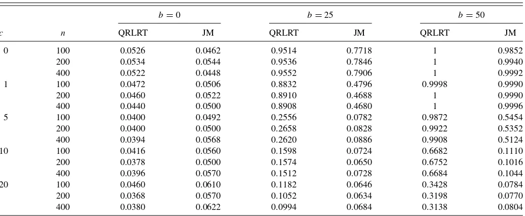
Table 2. Rejection rates for testingH0:β=0. Trueβ=
b√1−ρ2
n ,ρ= −0.98,α=1− c
n, nominal size=5%, 5000 replications
b=0 b=25 b=50
c n QRLRT JM QRLRT JM QRLRT JM
0 100 0.0526 0.0462 0.9514 0.7718 1 0.9852
200 0.0534 0.0544 0.9536 0.7846 1 0.9940
400 0.0522 0.0448 0.9552 0.7906 1 0.9992
1 100 0.0472 0.0506 0.8832 0.4796 0.9998 0.9990
200 0.0460 0.0522 0.8910 0.4688 1 0.9990
400 0.0440 0.0500 0.8908 0.4680 1 0.9996
5 100 0.0400 0.0492 0.2556 0.0782 0.9872 0.5454
200 0.0400 0.0500 0.2658 0.0828 0.9922 0.5352
400 0.0394 0.0568 0.2620 0.0886 0.9908 0.5124
10 100 0.0416 0.0560 0.1598 0.0724 0.6682 0.1110
200 0.0378 0.0500 0.1574 0.0650 0.6752 0.1016
400 0.0396 0.0570 0.1512 0.0728 0.6684 0.1044
20 100 0.0460 0.0610 0.1182 0.0646 0.3428 0.0784
200 0.0368 0.0570 0.1052 0.0634 0.3198 0.0770
400 0.0380 0.0622 0.0994 0.0684 0.3138 0.0804
in Theorem 3 with the test proposed in Jansson and Moreira (2006) (henceforth, JM). The data were generated from
Yt =βXt−1+ut
Xt =αXt−1+vt
α=1−c
n
ut
vt
iid ∼N
0,
1 ρ
ρ 1
,
where the intercept in each equation was set to zero without loss of generality, since our test is location invariant. As mentioned earlier in Section 3, initial simulation results showed that for a given pair (ρ, δ), the sup-bound critical value was qρ,δ(0),
that is, the supremum, overc, of the critical value was attained atc=0. Hence, for each replication, we first estimatedρ and then usedqρ,δˆ (0) as the critical value for our test. Furthermore,
since Chen and Deo (2010) reported that the iterated WLSRL estimates, obtained by using the first step WLSRL estimates in the weight functionWn, have better finite sample behavior, we
computed the QRLRT using these iterated WLSRL estimates. InTable 2, we compare our test procedure with JM’s condi-tional test forρ= −0.98. This large negative value ofρ was chosen to reflect the kind of values observed empirically (see Chen and Deo 2006). Simulation studies not reported here for
other values ofρ yielded results similar in nature to those re-ported here for ρ= −0.98. The sample sizen was set to be 100, 200, and 400 withc=0,1,5,10,and 20. Following JM’s set-up, the parameterβwas set to beb
√ 1−ρ2
n , whereb=0,25,
and 50. The rejection rates whenb=0 correspond to the size of the tests and whenb=25 and 50, to the power against lo-cal alternatives. Not surprisingly, it is seen from the table that the size of our test is slightly below the nominal level whenc takes large value, since QRLRT is asymptotically conservative. However, despite the conservative size, the power of our test is uniformly higher than that of the JM test, with the power gains being very substantial at times.
In Table 3, we provide, for comparison, simulation results for the configuration presented in Table II on page 702 of JM. Following the settings in Table II of JM, the correlationρ is set to −0.5 and 0.5, while the sample size is set atn=1000 with 500 replications. Once again, it is seen that the QRLRT maintains size while delivering power that is either identical to or higher than that of the JM test, with several power gains being very substantial.
Table 3. Rejection rates for testingH0:β=0. Trueβ=
b√1−ρ2
n ,α=1− c
n, nominal size=5%,n=1000, 500 replications
c c=0 c=5 c=10 c=15
ρ b QRLRT JM QRLRT JM QRLRT JM QRLRT JM
–0.5 0 0.040 0.054 0.042 0.058 0.056 0.042 0.046 0.066
5 0.488 0.424 0.186 0.102 0.138 0.076 0.112 0.080
10 0.892 0.826 0.620 0.338 0.438 0.180 0.316 0.154
15 0.990 0.946 0.904 0.702 0.772 0.392 0.646 0.230
0.5 0 0.062 0.046 0.052 0.036 0.064 0.018 0.058 0.022
5 0.398 0.412 0.196 0.132 0.150 0.054 0.114 0.040
10 0.728 0.602 0.504 0.220 0.372 0.122 0.300 0.088
15 0.908 0.720 0.746 0.274 0.622 0.196 0.508 0.082
530 Journal of Business & Economic Statistics, October 2013
APPENDIX A: MODEL WITH AN AR (p) REGRESSOR
We start by defining some notation. For t =p+1, . . . , n
and any time seriesζt, we will denote the corresponding sample
mean corrected series and its lag series as,
ζt,μˆ =ζt−
Furthermore, denote the series with the first observation subtracted as, ζs,d =ζs−ζ1, s=1, . . . , n, as before. Define tively, the WLSRL estimator
( ˆβWLS,βˆWLS,γˆWLS′ )
the WLSRL estimator underH0:β0is given by
Throughout this appendix, we will use the summation nota-tion!t for
!n
t=2unless stated otherwise.
Proof of Theorem 1. Without loss of generality, we will prove forβ =0. Following from Phillips (1987), Phillips and Magdalinos (2007), and Giraitis and Phillips (2012),
Using the matrix inversion formulas and letting
ηn=
With detailed algebraic calculation and writingut =ρvt+et,
( ˆβWLS, αˆWLS−α0)′=(Sn+ρˆTn, Tn)′+Rn′, (B.2)
Corollary 2. The theorem follows from Giraitis and Phillips (2012), the theorem follows from Phillips (1987) and Phillips
and Magdalinos (2007).
Proof of Lemma 1. The restricted estimate ofαin (3.1) is
ˆ
The remainder term R0
n=Op(1/n) ifλ∈[0,1/2] andR0n=
Op(1/ kn√n) if λ∈[1/2,1]. The limiting distribution of
( ˆα0WLS−α0follows from from (B.4) and Lemma 3.
Proof of Theorem 2. We will prove only forQ, the proof
ofLwill follow by the same proof in combination with Lemma 2 and Corollary 2. For algebraic convenience, we use the fol-lowing notations:
by (B.1), Lemma 2 and Corollary 2. With a Taylor expansion of
Qn,
532 Journal of Business & Economic Statistics, October 2013
The limiting distribution of n follows from Lemmas 4
and 5 .
Proof of Theorem 4. Let βn=b/√nkn and ˆαβ be the
WLSRL estimator ofαfor fixedβ. Now,
0= ∂Qn(β0,α, βˆ 0)
We get, from the above equation,
ˆ
with β0 being replaced by βn, thus, together with the above
equation,
Plugging the above equations into (B.5) and ignoring the smaller order terms,
The theorem follows from Lemmas 4 and 5 .
Lemma 2. LetWn(ρ, β, α) be defined as (Corollary2.2) and
Proof. With a few algebraic steps,
Wn(ρ, β, α)=
and the determinant ofW−1
n (ρ, β, α),
The lemma follows immediately.
Corollary 1. LetWn(ρ, β, α) be defined as2.2, then the
ex-pressions ofWnin Lemma 2 hold for any value ofβ.
Corollary 2. Let ˆρ be a consistent estimate ofρ and ˆβ be a consistent estimate ofβ. Furthermore, let ˆαbe a consistent estimate of α such that n(1+λ)/2
Lemma 3. Let w22 be the (2,2)th entry of Wn(α, β, ρ) in
(2.2),
t
Xt−1,μˆvt,μˆ +
w22*!s,tXs−1,dXt,d −α
!
sXs−1,d
2+
n−1
=
!
tXt−1,μˆvt,μˆ +Op(nλ), λ∈[0,1/2]
!
tXt−1vt+Op(√n), λ∈[1/2,1]
and
t
X2t−1,μˆ +w22 !
sXs−1,d
2
n−1
=
!
tX2t−1,μˆ +Op(n2λ), λ∈[0,1/2]
!
tX
2
t−1+Op(n1/2+λ), λ∈[1/2,1]
.
Proof. The lemma follows from Lemma 2 that w22 = O(n−1+2λ
), when λ∈[0,1/2] andw22 =1+o(1), whenλ∈
(1/2,1], and the fact that
s,t
Xs−1,dXt,d −α
s
Xs−1,d
2
=
s
(Xs−X1)
t
{vt−(1−α)X1}
and
s
Xs−1,d
2 =
s
Xs−1 2
−(n−1)X1
×
s
Xs−1+(n−1)2X21.
Lemma 4. Letet =ut−ρvt and
Sn= !
tXt−1,μˆet,μˆ !
tXt2−1,μˆ ,
then
nknSn−−−→ D
⎧ ⎪ ⎪ ⎪ ⎪ ⎪ ⎪ ⎨ ⎪ ⎪ ⎪ ⎪ ⎪ ⎪ ⎩
N(0,(1−ρ2)(1−α2)), αis fixed, kn=1
N(0,2c(1−ρ2)), α=1−c/ kn, kn=nλ, λ∈(0,1)
Jc,μ2 (r)dr −1/2
α=1−c/n .
1−ρ2Z,
Proof. Sinceet,μˆ is independent ofXt−1,μˆ, !
tXt−1,μˆet,μˆ
(1−ρ2)!
tXt2−1,μˆ
--Xt−1,μˆ ⇒Z.
When α is fixed, n−1!
tX
2
t−1,μˆ →p (1−α2)−1. When
α=1−c/nλwithλ
∈(0,1), (nkn)−1
!
tX
2
t−1→p 1/2cfrom
Phillips and Magdalinos (2007), and (n−1)−1!
tXt−1= Op(k2n/n) from Giraitis and Phillips (2012), thus
1
nkn
t
X2t−1,μˆ = 1 nkn
t
X2t−1(1+op(1))−→p
1 2c.
Furthermore, when α=1−c/n, n−2!
tX
2
t−1,μˆ ⇒
Jc mu(r)2dr.
Lemma 5. Letw22be the (2,2)th entry ofWn,and
Tn= !
tXt−1,μˆvt,v+nw−221
!
s,tXs−1,d(Xt,d−α0Xt−1,d)
!
tXt2−1,μˆ +
w22
n−1 !
sXs−1,d
2 ,
then
nknTn−−−→ D
×
⎧ ⎪ ⎪ ⎨ ⎪ ⎪ ⎩
N(0,(1−α2)), α is fixed, k
n=1
N(0,2c), α=1−c/ kn, kn=nλ, λ∈(0,1)
Jc(r)2dr τc, α=1−c/n .
Proof. The lemma follows from Lemma 3, Phillips (1987), and Phillips and Magdalinos (2007).
ACKNOWLEDGMENTS
Chen’s research was supported by NSF grant DMS-1007652.
[Received January 2013. Revised June 2013.]
REFERENCES
Bobkoski, M. J. (1983), “Hypothesis Testing in Nonstationary Time Series,” Ph.D. Thesis, The University of Wisconsin. [527]
Cavanagh, C. L., Elliott, G., and Stock, J. H. (1995), “Inference in Models With Nearly Integrated Regressors. Trending Multiple Time Series,”Econometric Theory, 11, 1131–1147. [527,528]
Chen, W., and Deo, R. (2009a), “Bias Reduction and Likelihood Based Almost-Exactly Sized Hypothesis Testing in Predictive Regressions Using the Re-stricted Likelihood,”Econometric Theory, 25, 1143–1179. [525,526] ——— (2009b), “The Restricted Likelihood Ratio Test at the Boundary in
Autoregressive Series,”Journal of Time Series Analysis, 30, 618–630. [526] ——— (2010), “Weighted Least Squares Approximate Restricted Likelihood Estimation for Vector Autoregressive Processes,”Biometrika, 97, 231–237. [525,526,529,530]
——— (2012), “The Restricted Likelihood Ratio Test for Autoregressive Pro-cesses,”Journal of Time Series Analysis, 33, 325–339. [526]
Giraitis, L., and Phillips, P. C. B. (2012), “Mean and Autocovariance Function Estimation Near the Boundary of Stationarity,”Journal of Econometrics, 169, 166–178. [526,531,533]
Jansson, M., and Moreira, M. (2006), “Optimal Inference in Regression Models With Nearly Integrated Regressors,”Econometrica, 74, 681–714. [525,529] Larsson, R. (1995), “The Asymptotic Distributions of Some Test Statistics in Near-Integrated AR Processes,”Econometric Theory, 11, 306–330. [527] Phillips, P. C. B. (1987), “Towards a Unified Asymptotic Theory for
Autore-gression,”Biometrika, 74, 535–547. [527,531,533]
Phillips, P. C. B., and Magdalinos, T. (2007), “Limit Theory for Moderate Deviations From a Unit Root,”Journal of Econometrics, 136, 115–130. [531,533]