Full Terms & Conditions of access and use can be found at
http://www.tandfonline.com/action/journalInformation?journalCode=ubes20
Download by: [Universitas Maritim Raja Ali Haji] Date: 12 January 2016, At: 17:34
Journal of Business & Economic Statistics
ISSN: 0735-0015 (Print) 1537-2707 (Online) Journal homepage: http://www.tandfonline.com/loi/ubes20
Do Leading Indicators Lead Peaks More Than
Troughs?
Richard Paap, Rene Segers & Dick van Dijk
To cite this article: Richard Paap, Rene Segers & Dick van Dijk (2009) Do Leading Indicators
Lead Peaks More Than Troughs?, Journal of Business & Economic Statistics, 27:4, 528-543, DOI: 10.1198/jbes.2009.07061
To link to this article: http://dx.doi.org/10.1198/jbes.2009.07061
Published online: 01 Jan 2012.
Submit your article to this journal
Article views: 138
View related articles
Do Leading Indicators Lead Peaks
More Than Troughs?
Richard PAAP, Rene SEGERS, and Dick
VANDIJK
Econometric Institute and Tinbergen Institute, Erasmus University Rotterdam, NL-3000 DR Rotterdam, The Netherlands (paap@ese.eur.nl;rsegers@ese.eur.nl;djvandijk@ese.eur.nl)
We develop a novel Markov switching vector autoregressive model to investigate the possibility that lead-ing indicators have different lead times at business cycle peaks and at troughs. In this model, coinci-dent and leading indicators share a common Markov state process, but their cycles are nonsynchronous, with the nonsynchronicity varying across regimes. An application shows that on average the Conference Board’s Composite Leading Index leads the Composite Coincident Index by nearly 1 year at peaks but by only 1 quarter at troughs. Allowing for asymmetric lead times yields improved real-time dating and forecasting of business cycle turning points.
KEY WORDS: Bayesian inference; Business cycle; Leading indicator; Markov switching; Real-time data.
1. INTRODUCTION
Reliable leading indicators of the business cycle are of great importance for policy makers, firms, and investors. Thus it is not surprising that economists have embarked on an intensive quest for such leading indicators, beginning with the initial at-tempts ofMitchell and Burns (1938)for the U.S. economy. This research has provided much insight into the construction, use, and evaluation of leading indicators (seeMarcellino 2006for a recent survey).
Reliability of a leading indicator variable includes such as-pects as consistency and timeliness. Consistency refers to the property that a leading indicator should systematically give an accurate indication of the future course of the economy and should not produce false turning point signals too frequently, for example. Timeliness means that to be useful, a leading indi-cator variable should have a considerable lead time with respect to business cycle turning points. Most of the currently popular leading indicator variables are believed to have a lead time of between 6 and 18 months. At the same time, many of these vari-ables appear to have a considerably longer lead time at business cycle peaks than at troughs; for example, the Composite Index of Leading Indicators (CLI) currently published by The Con-ference Board has led cyclical downturns in the economy by 8–20 months and upturns by 1–10 months in the post-World War II period (The Conference Board 2001).
In this article we develop a formal approach to investigate whether leading indicator variables have different lead times at peaks and at troughs. For this purpose, we propose a novel Markov switching vector autoregressive model in which eco-nomic growth and leading indicator variables share a common nonlinear cycle determined by a single Markov process, but such that their regime-switching is not exactly synchronous with the length of the displacement or lead/lag time varying across the different regimes. We follow a Bayesian approach for estimating the model parameters, obtaining posterior results through flexible Markov chain Monte Carlo techniques. The ad-vantage of a Bayesian analysis of the model is that it allows us to treat the lead/lag times as unknown parameters. We can use their posterior distributions to conduct statistical inference on the asymmetry of the lead/lag structure at peaks and troughs.
We provide an empirical application involving the Confer-ence Board’s monthly Composite Coincident Index (CCI) and CLI over the period January 1959–June 2007. We find that on average the CLI leads CCI by nearly 1 year at peaks but by only 1 quarter at troughs. This suggests that in terms of timeli-ness, the CLI is most useful for signaling oncoming recessions. The posterior results provide convincing evidence favoring the presence of a nonsynchronous common cycle with asymmetric lead times. The Bayes factor relative to an alternative specifi-cation with equal lead times at cyclical downturns and upturns is very large. This also applies to models with synchronous cy-cles and with independent cycy-cles in the different variables. In addition, the CLI is more consistent and more timely in terms of signaling oncoming recessions when embedded in the gen-eral model specification. To examine the practical usefulness of allowing for asymmetric lead times, we conduct a business cycle dating and forecasting exercise for the period December 1988–July 2007, using real-time data for both the CLI and CCI. We find that allowing for asymmetric lead times leads to more timely and precise identification of peaks and troughs for the 1990–1991 and 2001 recessions, as well as more accurate out-of-sample forecasts of turning points and CCI growth rates.
The article is organized as follows. In Section2we introduce our novel Markov switching vector autoregressive model. We also describe (nested) alternative specifications, which allow for a nonsynchronous common cycle but with identical lead times at all possible regime switches, for a synchronous common cy-cle, and for independent cycles. To facilitate model interpreta-tion, we focus on the bivariate case, in which both economic growth (or the coincident indicators) and the leading indica-tors are represented by a single variable. We provide details of the Bayesian approach for parameter estimation and infer-ence in Section3. In Section4we discuss the empirical results based on estimating the different model specifications over the complete sample period. In Section5we consider the real-time
© 2009American Statistical Association Journal of Business & Economic Statistics October 2009, Vol. 27, No. 4 DOI:10.1198/jbes.2009.07061
528
performance of the alternative cycle representations in terms of identifying peaks and troughs and also with respect to fore-casting turning points and CCI growth. Finally, we conclude in Section6.
2. MODEL SPECIFICATION
Our point of departure is the assumption that the cycles in both the coincident indicator of aggregate economic activity (which can be an index as well as an individual measure, such as industrial production or GDP) and the leading indicator con-sist of two regimes (although extensions to multiple regimes are possible, as discussed later), designated “recession” and “expansion,” which are characterized by different mean growth rates of these variables. To make this precise, lety1,tandy2,t
de-note the growth rates of the coincident and leading indicators, respectively, in periodt. Consider the unobserved binary ran-dom variabless1,t ands2,t, wheresj,t takes value 0 in the case
whereyj,tis in expansion and 1 in the case whereyj,tis in the
re-cession regime. The mean growth rate conditional on the state
sj,t is denoted as μj,sj,t ≡E[yj,t|sj,t], for j=1,2, where
typi-callyμj,1<0< μj,0 such that recessions and expansions cor-respond to periods with negative and positive average growth, respectively. The properties of s1,t ands2,t determine the
re-lationship between the cyclical behavior of the coincident and leading indicators; we return to these properties in detail later. For the moment, it is sufficient to say that they are assumed to be homogeneous first-order Markov processes. Finally, assum-ing first-order autoregressive dynamics in the demeaned growth rates, we arrive at the specification
y1,t−μ1,s1,t =φ1,1
andt2. We can write this model in vector notation as
The Markov switching vector autoregressive (MS-VAR) model in (3) obviously needs to be completed by specifying the exact dynamic properties ofs1,t ands2,t. We consider four
different specifications, which allow for varying degrees of in-terrelation between the cycles in the coincident and leading indicators. First, an extreme viewpoint would be to assume that
these cycles are completely independent. In this case, the state vectors s1,t and s2,t can be defined as two independent
first-order, two-state homogeneous Markov processes with transi-tion probabilities
Pr[sj,t=0|sj,t−1=0] =pj and
(5) Pr[sj,t=1|sj,t−1=1] =qj, j=1,2.
Second, the opposite extreme would be to assume that the variablesy1,tandy2,tshare a common business cycle, which is
obtained by imposing
s2,t=s1,t for allt. (6)
Consequently, a single underlying Markov process with tran-sition probabilitiespandq can be used to model the business cycle. (SeeKrolzig 1997,Paap and van Dijk 2003, andChauvet and Hamilton 2006for extensive treatments of this model spec-ification.)
Third, a more subtle approach, as proposed byHamilton and Perez-Quiros (1996), is to assume that although the coincident and leading indicators share the same business cycle, the cycle of the leading indicators leads or lags the cycle of the coincident variable byκperiods, that is,
s2,t=s1,t+κ forκ∈Z. (7)
Note that positive values of κ correspond to the situation in which the cycle of y2,t leads the cycle of y1,t by κ periods,
whereas negative values correspond to a lag of|κ|periods. We may treat the lead timeκ as an unknown parameter to be esti-mated.
As discussed in Section1, stylized facts demonstrate that on average, leading indicators have a longer lead time when en-tering a recession than when enen-tering an expansion. To capture this phenomenon, we consider a new specification of the state parameters accompanying the MS-VAR model (3) such thats2,t
leadss1,t byκ1periods at peaks and byκ2periods at troughs. This can be formalized by definings2,tas
s2,t=
To demonstrate that this specification indeed gives rise to the desired asymmetric lead times, consider the case where
κ1≤κ2. Defining s2,t as the product from s1,t+κ1 to s1,t+κ2
essentially implies that recessions in y2,t start κ1 periods be-fore recessions iny1,tand endκ2periods earlier. Consequently, recessions in y2,t are |κ2−κ1| periods shorter than reces-sions in y1,t. In contrast, if κ1> κ2, then recessions in y2,t
are|κ1−κ2|periods longer than recessions iny1,t. Obviously,
lengthening the recession periods is equivalent to shortening the expansions; for that reason, we defines2,tin (8) in terms of the
product over(1−s1,t)in this case.
Note that the specification ofs2,t in (8) embeds the
specifi-cations with a synchronous common cycle (κ1=κ2=0) and with a nonsynchronous common cycle with symmetric lead/lag times at peaks and troughs (κ1=κ2) as special cases. This facil-itates testing for the degree of interrelation between the two cy-cles. The four specifications of the state vectorssj,tforj=1,2
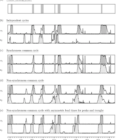
discussed earlier are given in Table1.
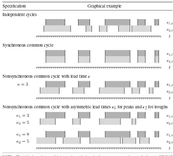
Table 1. Possible cycle interrelationships
Specification Graphical example
Independent cycles
Synchronous common cycle
Nonsynchronous common cycle with lead timeκ
Nonsynchronous common cycle with asymmetric lead timesκ1for peaks andκ2for troughs
NOTE: The table shows four possible types of specifications for the processess1,tands2,tin the bivariate MS-VAR
model (3), with different types of relationship between the cycles iny1,tandy2,t: (a) independent cycles as implied by (5),
(b) a synchronous common cycle as in (6), (c) a nonsynchronous common cycle with identical lead/lag timeκat peaks and troughs as in (7), and (d) a nonsynchronous common cycle with different lead/lag timesκ1at peaks andκ2at troughs as in
(8). The dark- and light-gray-shaded areas correspond to recession periods iny1,tandy2,t, respectively.
The bivariate MS-VAR(1) model in (3) may be extended in several directions to make it more realistic and useful in em-pirical practice. First, we may want to consider multiple coin-cident indicator variables, based on the original idea of Burns and Mitchell (1946, p. 3) that the business “cycle consists of expansions (and recessions) occurring at about the same time in many economic activities.” We also may use the information in the recession indicator of the National Bureau of Economic Research (NBER) as inIssler and Vahid (2006), although the relatively large publication lag of this indicator makes it less useful for forecasting. Similarly, including multiple leading in-dicator variables may be beneficial, because different recessions have different sources and characteristics and thus may be sig-naled by different leading indicators (see, e.g.,Stock and Wat-son 2003). This may be accommodated by taking yj,t to be a
(mj×1)vector forj=1,2, such that the model includes m1 coincident indicators and m2 leading indicators. In the event that bothm1>1 andm2>1, clearly defining the relationships between the states sj,t,j=1, . . . ,m1+m2 directly as in (8) may be cumbersome, because now there are m1×m2 differ-ent lead/lag times to consider. A possible solution then is to use a dynamic factor structure (as inChauvet 1998), where all coin-cident and leading indicators are related with a certain lead/lag time to a latent common factor that exhibits regime-switching behavior.
Second, the model may be extended to incorporate higher-order dynamics in the coincident and leading indicators. For
any lag orderk≥0, the general MS-VAR model reads
Y
t−MSt=1Yt−1−MSt−1+ · · ·
+kY
t−k−MSt−k+Et
=
k
i=1 iY
t−i−MSt−i+Et, (9)
or, using lag polynomial notation
(L)Zt=(I−1L− · · · −kLk)Zt=Et, (10) whereZt=Yt−MSt.
A third possible extension of the model concerns the possi-bility of multiple regimes. For example, several applications of Markov switching models to U.S. GDP have found that allow-ing for a third regime to capture the so-called “bounce-back ef-fect” (i.e., a short period of rapid recovery following recessions) considerably improves the description of the cyclical dynamics of output (see, e.g.,Sichel 1994;Boldin 1996; Clements and Krolzig 2003). In the case of multiple regimes, specifying the lead/lag structure of the regime-switches for the different vari-ables in the model may be complicated and must be done with care.
Fourth, a model specification in which the transition prob-abilities of the Markov processessj,t, for j=1,2, depend on
observed explanatory variables may be considered (see, e.g.,
Diebold, Lee, and Weinbach 1994;Filardo 1994;Diebold and Rudebusch 1996).
Fifth and finally, regime-dependent heteroscedasticity and correlations among the shocksEt may be captured by
replac-ing the assumptionEt∼N(0,)in (3) byEt|St∼N(0,St).
In the empirical application that follows, we consider another type of dynamics in the error (co)variances to accommodate the effects of the “Great Moderation,” the large and persis-tent decline in the volatility of U.S. macroeconomic time series since the mid-1980s (see, e.g.,McConnell and Perez-Quiros 2000;Sensier and van Dijk 2004;Herrera and Pesavento 2005). Specifically, we allow for a single structural break in the covari-ance matrix ofEt: whereI[·]denotes the indicator function, taking value 1 if the condition in brackets is true and 0 otherwise, and0 and1 are(2×2)covariance matrixes. We treat the break pointτ as an unknown parameter to be estimated.
3. ESTIMATION AND INFERENCE
Parameter estimation and inference on the regimes in MS-(V)AR models is commonly done using maximum likelihood coupled with the EM algorithm (see Hamilton1989,1994for details). But because we wish to conduct inference on the dis-crete lead/lag time parametersκ1 andκ2 in (8), a frequentist approach is not feasible. Thus we adopt a Bayesian approach. In Section3.1we derive the likelihood function of the model, and in Sections3.2and3.3we discuss prior specification and posterior simulation.
3.1 The Likelihood Function
We first derive the complete data likelihood function. We fo-cus on the derivation for the bivariate MS-VAR model (9) with asymmetric lead/lag structure as given in (8). The likelihood of the other specifications can be derived similarly.
FollowingHamilton (1989)andPaap and van Dijk (2003), we replaceMSt by
MSt=Ŵ0+Ŵ1⊙St, (12)
where⊙denotes the Hadamard or element-by-element product andSt is as given in (4) with (8). ThusŴ0=(μ1,0, μ2,0)′and
The conditional density ofYt for this model given the past
and current statesSt
whereEtfollows from (13). Thus the complete data likelihood
function for model (13) conditional on the firstkobservations
Ykequals
the number of transitions from state ito statej. The uncondi-tional likelihood functionL(YT|Yk,θ)can be obtained by sum-ming over all possible realizations ofs1,
L(YT|Yk,θ)= follows directly from (15). If we have separate cycles for the two series inYt, then we need to extend (15) with the likelihood
contribution of the second cycle in a straightforward manner.
3.2 Prior Specification
We opt for a prior specification that is relatively uninforma-tive compared with the information in the likelihood. For the transition probabilitiesp andq, we take independent and uni-formly distributed priors on the unit interval(0,1)
f(p)=I[0<p<1] and f(q)=I[0<q<1]. (17) Under flat priors for p and q, special attention must be paid to the priors for Ŵ0 andŴ1. It is easy to show that the like-lihood has the same value if we switch the role of the states, switchκ1withκ2, and change the values ofŴ0,Ŵ1,p, andqto Ŵ0+Ŵ1,−Ŵ1,q, andp, respectively (seeFrühwirth-Schnatter 2001). This complicates proper posterior analysis if we are in-terested in the values ofŴ0andŴ1(see alsoGeweke 2007for a discussion). FollowingPaap and van Dijk (2003), we take pri-ors forŴ0andŴ1on subspaces which identify the regimes, that is,
Thus we impose that the growth rate μ for the first series is positive ifs1,t=0 and negative ifs1,t=1 (see alsoSmith and
Summers 2005for a discussion on this issue). For the model specification with two independent cycles (or, put differently, two independent Markov processes s1,t ands2,t), we take the
priors given in (17) for both sets of transition probabilities. In that case the prior forŴ0andŴ1as given in (18) is augmented with the additional restrictions Ŵ0,2>0 and Ŵ0,2+Ŵ1,2<0 to identify the regimes of y2,t. Note that Smith and Summers
(2005)are less restrictive and only impose that the diagonal el-ements ofŴ1+Ŵ0are smaller or equal to 0 and have no further restrictions on the diagonal elements ofŴ0.
For the shift parametersκj, we take a discrete uniform prior,
periods. The same prior is used for the lead timeκ in the model specification with a nonsynchronous common cycle but equal lead times at peaks and troughs based on (7).
For the autoregressive parameters, we use flat priors,
f(i)∝1 fori=1, . . . ,k−1, (20) and forj, we take the uninformative prior
f(j)∝ |j|−3/2 (21) forj=0,1. This prior results from a standard Wishart prior by letting the degrees of freedom approach 0 (seeGeisser 1965).
Finally, for the break parameterτ, we take a discrete uniform prior,
thus not allowing for a break in the first and lastbobservations of the sample period.
The joint prior for the model parametersf(θ)is given by the product of (17)–(22).
3.3 Posterior Distributions
The posterior distribution for the model parameters of the MS-VAR model is proportional to the product of the joint prior
f(θ)and the unconditional likelihood functionL(YT|Yk,θ). To obtain posterior results, we use the Gibbs sampling algorithm ofGeman and Geman (1984)along with the data augmentation method ofTanner and Wong (1987). The unobserved state vari-ables{St}T
t=1are simulated alongside the model parametersθ (see, e.g.,Albert and Chib 1993; McCulloch and Tsay 1994;
Chib 1996;Kim and Nelson 1999).
The Gibbs sampler is an iterative algorithm, where one con-secutively samples from the full conditional posterior distribu-tions of the model parameters. This produces a Markov chain that converges under mild conditions. The resulting draws can be considered a sample from the posterior distribution (see
Smith and Roberts 1993;Tierney 1994for details). In the Ap-pendixwe derive the full conditional posterior distributions re-sulting fromf(θ)L(YT,ST|Yk,θ)for the model specification
with asymmetric lead/lag structure.
4. EMPIRICAL RESULTS
We apply the MS-VAR models proposed in Section2to
ex-amine the lead times at business cycle peaks and troughs of the CLI as issued by The Conference Board. As a measure of economic activity we consider the Conference Board’s CCI, which comprises employment, industrial production, manufac-turing and trade sales, and personal income less transfer pay-ments. Both time series are transformed to monthly growth rates. The sample period runs from January 1959–June 2007.
The estimation results reported in this section use the revised data available in July 2007. In the next section we consider out-of-sample forecasting of turning points and CCI growth rates based on real-time data.
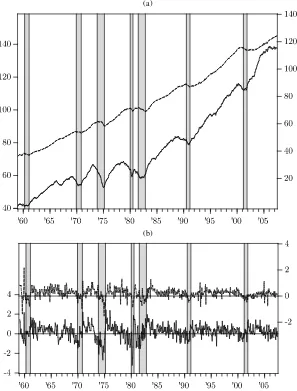
Figure 1 displays a time series plot of the log levels and monthly percentage growth rates of both series, together with the recession periods as determined by the NBER. In general, the leading index seems to have a similar cyclical pattern as the coincident index, but with turning points clearly occurring earlier. In addition, the visual evidence in Figure1already sug-gests that the CLI turning points have a longer lead time for business cycle peaks than for troughs. We apply the four dif-ferent specifications of the Markov switching model discussed in Section2to investigate formally whether this indeed is the case, and also to determine by how many periods the leading in-dicator actually is leading at peaks and troughs. In addition, for comparison, we include a linear VAR, which can be obtained from (9) by settingMSt =Mfor allt.
We estimated all five models without and with a single struc-tural break in volatility, as in (11). We found that the marginal likelihoods are clearly larger for the models with a structural break compared with the models without a structural break, pro-viding strong posterior evidence for a structural break in volatil-ity. The models with and without volatility break are quite sim-ilar in other respects, however. For those reasons, and also to save space, here we report results for the models that incorpo-rate a volatility break. Detailed results for the models that do not allow for a structural break in volatility are available on re-quest.
To perform inference, we used the Bayesian approach as dis-cussed in Section3, with the prior specifications given in Sec-tion3.2. We set the parametersc1andc2 in the priors for the lead/lag timesκ1 andκ2equal to 18, implying that we allow for a maximum nonsynchronicity of 1–1/2 years in the cycles of both series. The parameterbin the prior for the break date is set equal to 6, so that we do not allow for a break in the (co-)variances in the first and last six observations. We con-sider several specifications for the autoregressive dynamics in (9). Unreported Bayes factors based on moderately informa-tive priors onindicate that a lag orderk=1 with additional restrictionsφ1,1=φ2,1=0 is most appropriate (seeHamilton
and Perez-Quiros 1996for a similar specification). Thus only lagged CLI growth rates enter the equations for both CCI and CLI.
Posterior results of the five estimated models are shown in Table2, based on 100,000 simulations after a burn-in period of 10,000 simulations. The first panel of the table shows that in the linear VAR model, the posterior means of the average monthly growth rate of CLI and CCI are roughly equal over the sample period (0.21% and 0.20%, respectively); however, the posterior standard deviation of the growth rate of the leading index is substantially higher. In the MS-VAR models we see clear dif-ferences in the average growth rates during periods of reces-sion and expanreces-sion. Depending on the model specification, for the CCI series, the posterior means of the average growth rates are between 0.26% and 0.30% during expansions and between
−0.26% and −0.12% during recessions. The posterior mean of the probability of staying in an expansion regime is about 0.97, whereas the probability of staying in a recession regime is considerably lower, about 0.87 on average. This obviously
(a)
(b)
Figure 1. Time series plots of the CCI (- - - -) and CLI ( ), monthly observations for the period January 1959–June 2007.
reflects the fact that recessions typically last shorter than reces-sions. Based on these average transition probability estimates, the expected duration of recessions is between 7 and 8 months, compared with 33 months for expansions. Note that there is much more variability in the posterior means of the probabil-ity of staying in a recession than for the probabilprobabil-ity of stay-ing in an expansion across the different model specifications; in particular, the probability of staying in recession varies be-tween 0.83 for the asymmetric nonsynchronous cycle specifica-tion and 0.90 for the specificaspecifica-tion with independent cycles.
The fourth panel of Table2shows that in the model with a nonsynchronous common cycle (7), the posterior mean of the lead time of the CLI is around 9 months. This is considerably longer than the lead time of 1 quarter reported byHamilton and Perez-Quiros (1996). This large discrepancy can be attributed to substantial differences in methodology. In particular,Hamilton and Perez-Quiros (1996) obtained their results for quarterly GDP and CLI data on a shorter sample period using frequentist inference methods. In the novel model specification allowing for asymmetric lead/lag timesκ1andκ2, the posterior mean of the lead time is about 11.7 months at peaks and 3.8 months at troughs. This confirms the informal visual evidence in Figure1
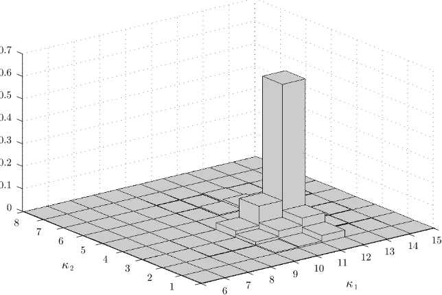
that the CLI signals oncoming recessions earlier than expan-sions. Figure2displays the posterior distribution of theκj
para-meters, forj=1,2 in this model specification, showing that the posterior mode isκ1=12 andκ2=4. The posterior probability that κ1=κ2 is only 0.02, providing complementary evidence that the lead times at the start of recessions and expansions re-ally are different.
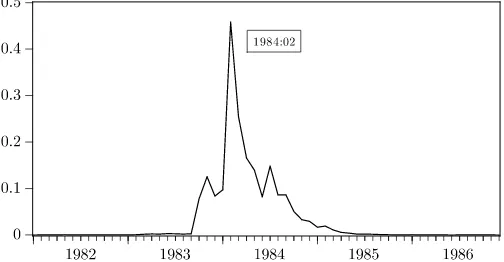
The bottom panel of the table shows that the posterior mode of the breakpoint parameterτ is 1984:02 in all model specifica-tions, which corresponds with the breakpoint estimate for GDP volatility reported by McConnell and Perez-Quiros (2000), among others. Figure 3 displays the posterior density of the break parameter for the model with an asymmetric lead/lag structure for the period January 1982–December 1986. Almost all posterior mass is located in the years 1983 and 1984. In the MS-VAR model with asymmetric lead/lag times, the posterior means of the variances are such that for CCI, the variance after the break is about 43% of the variance before the break. For the leading indicator, the reduction in variance also is very large, at 47%. The posterior means of the correlation between the CCI and CLI growth rates are 0.55 before the break and 0.40 after the break. This suggests that the strength of the co-movement between the series declined as well.
Table 2. Posterior means and standard deviations (in parentheses) of parameters in linear and MS-VAR models with volatility break
MS-VAR
Asymmetric
Independent Synchronous Nonsynchronous nonsynchronous
Linear VAR cycles common cycle common cycle common cycle
Growth rates μ1,0 0.197 (0.016) 0.304 (0.019) 0.274 (0.018) 0.281 (0.018) 0.262 (0.014)
μ1,1 −0.118 (0.042) −0.208 (0.055) −0.138 (0.063) −0.257 (0.043)
μ2,0 0.214 (0.040) 0.334 (0.037) 0.216 (0.049) 0.332 (0.051) 0.373 (0.036)
μ2,1 −0.839 (0.118) −0.039 (0.044) −0.295 (0.129) −0.296 (0.061)
Transition p1 0.972 (0.011) 0.966 (0.011) 0.964 (0.012) 0.973 (0.008)
probabilities q1 0.904 (0.038) 0.841 (0.053) 0.870 (0.044) 0.833 (0.046)
p2 0.974 (0.011)
q2 0.797 (0.080)
Dynamics φ1,2 0.105 (0.022) 0.121 (0.026) 0.096 (0.024) 0.068 (0.026) 0.047 (0.024)
φ2,2 0.376 (0.041) 0.297 (0.053) 0.394 (0.041) 0.279 (0.058) 0.217 (0.043)
Lead/lag times κ1 9.228 (2.712) 11.710 (0.637)
κ2 3.794 (0.553)
Covariance ω11,1 0.180 (0.015) 0.935 (0.576) 0.132 (0.012) 0.140 (0.014) 0.136 (0.012)
matrixes ω21,2 0.548 (0.046) 1.172 (0.791) 0.543 (0.046) 0.482 (0.050) 0.464 (0.040)
ρ1 0.413 (0.049) 0.711 (0.182) 0.478 (0.052) 0.520 (0.051) 0.547 (0.046)
ω12,1 0.069 (0.006) 0.087 (0.006) 0.051 (0.005) 0.055 (0.006) 0.060 (0.006)
ω22,2 0.255 (0.022) 0.310 (0.022) 0.261 (0.024) 0.229 (0.024) 0.220 (0.020)
ρ2 0.407 (0.051) 0.535 (0.037) 0.460 (0.057) 0.423 (0.060) 0.403 (0.054)
Most likely break date τ 1984:02 1984:02 1984:02 1984:02 1984:02
Log-marginal likelihood –671.6 −656.6 −656.7 −635.8 −622.8
NOTE: The table presents posterior means and standard deviations (in parentheses) of parameters in linear and MS-VAR models with a single structural change in the covariance matrixes [as in (11)], estimated for monthly growth rates of the CCI and CLI over the period January 1959–June 2007. The parametersρ1andρ2denote the correlation between the CCI and CLI growth rates before the break date and after the break date. The most likely break date is defined as the mode of the posterior distribution ofτ. The four specifications for the processess1,tands2,tin the bivariate MS-VAR model are such that CCI and the CLI have (a) independent cycles as implied by (5), (b) a synchronous common cycle as in (6), (c) a
nonsynchronous common cycle with identical lead/lag timeκat peaks and troughs as in (7), and (d) a nonsynchronous common cycle with different lead/lag timesκ1at peaks andκ2at
troughs as in (8). Posterior results are based on 100,000 simulations. The number of burn-in simulations is 10,000.
Figure 2. Joint posterior density of the lead/lag parametersκ1andκ2. The graph presents the joint posterior density of the lead/lag parameters κ1andκ2in the MS-VAR model with a nonsynchronous common cycle with asymmetric lead/lag timesκ1at peaks andκ2at troughs as in (8) and a single structural change in the covariance matrix as in (11), estimated for monthly growth rates of the CCI and CLI for the period January 1959–June 2007.
Figure 3. Posterior density of the variance breakpoint parameterτ. The graph presents the posterior density of the variance break dateτ
(for the period January 1982–December 1986) in the MS-VAR model with a nonsynchronous common cycle with different lead/lag timesκ1
at peaks andκ2at troughs as in (8) and a single structural change in the covariance matrix as in (11), estimated for monthly growth rates of the CCI and CLI over the period January 1959–June 2007.
The bottom panel of the table also shows the log-marginal likelihoods of the five models. Because we have proper pri-ors on the transitions probabilities, we can compare the log-marginal likelihoods of the four Markov switching models to assess the appropriateness of the different cycle specifications. The log-marginal likelihood is clearly greater for the model with asymmetric lead/lag structure than for the other models. The log-Bayes factor compared with the nonsynchronous com-mon cycle specification is 13, providing strong posterior evi-dence for the more general specification with different lead/lag times at peaks and troughs.
We judge the different model specifications on their ability to signal turning points and to identify recession periods. Figure4
shows the posterior means of the state variables sj,t,j=1,2
for the four Markov switching models. The shaded areas indi-cate “recession periods,” defined as six consecutive months in which the posterior mean ofsj,texceeds 0.5. This corresponds
with the popular rule of thumb that the economy is in recession whenever economic growth is negative during two consecutive quarters. We emphasize that we do not propose this censoring rule as a formal means to identify business cycle regimes. For that purpose, it is better to consider the posterior probabilities of the state variables1,tfor the coincident indicator directly. We
compare the posterior means ofs1,twith the business cycle
ex-pansions and recessions as implied by the NBER turning points, thus assuming that the latter are correct. It is useful to note that the CCI consists of the same four monthly series closely mon-itored by the NBER business cycle dating committee. At the same time, the NBER of course also considers other indicators of economic activity, such as real GDP.
The bottom graph in Figure4reveals that the model with an asymmetric lead/lag time at peaks and troughs as in (8) does an excellent job identifying the regimes of the business cycle. For all of the official NBER-dated recessions that occurred dur-ing the sample period, the posterior mean ofs1,t is very close
to 1. In addition, no false recession signals are given except around 1967, which corresponds with a growth rate cycle reces-sion, according to the Economic Cycle Research Institute (see
http:// www.businesscycle.com). Comparing the graphs in pan-els (b)–(d) demonstrates the advantage of allowing for different
lead times at peaks and troughs in two different ways. First, the posterior probabilities obtained from the asymmetric lead time specification allow for much sharper inference concerning the business cycle regimes. Although the other specifications also identify all recessions that occurred during the sample period, their signal is more noisy in the sense that the posterior mean of
s1,t often lingers at values between 0 and 1. This is especially
noticeable for the two most recent recessions in 1990–1991 and 2001, for which the posterior means of s1,t in panels (b)–(d)
return to 0 much later than the official troughs in March 1991 and November 2001. In contrast, panel (e) shows a clear and timely signal of the end of these recessions, as the posterior mean ofs1,t drops to 0 close to these trough dates. Second, the
model with a nonsynchronous common cycle with an asymmet-ric lead/lag structure is more timely, in the sense that it signals oncoming recessions (by showing an increase in the probabil-ity thats2,t=1) quite a bit earlier than the other specifications.
This is most obvious for the model with a synchronous common cycle, which by definition is almost not able to identify a reces-sion before it actually occurs. In the model with independent cycles in panel (b), we do see a positive lead time ofs2,t but
only for the recessions in the first part of the sample period, be-fore the break in volatility. The 1990–1991 and 2001 recessions are completely missed by the CLI in this specification. Com-paring the two nonsynchronous common cycle specifications in panels (d) and (e) shows that the difference in the lead time at peaks is not very large, as suggested already by the difference in posterior means of just 2.5 months; see Table2. However, the signal provided by the state variable of the CLI (s2,t) is again
much more convincing in the asymmetric lead time specifica-tion.
5. REAL–TIME BUSINESS CYCLE DATING AND FORECASTING
The full-sample estimation results discussed in the previ-ous section demonstrate that using the CLI within a MS-VAR model delivers an accurate description of U.S. business cycle dynamics ex post. But the practical usefulness of leading indi-cator variables hinges crucially on their ability to signal changes in the business cycle ex ante. Furthermore, because both the CCI and CLI are subject to substantial revisions after their ini-tial release, a realistic assessment of this issue requires the use of real-time data that were actually available when the forecasts were supposed to be made. Two related aspects of real-time performance are of interest. First, we consider real-time busi-ness cycle dating, as described byChauvet and Piger (2008), and examine how quickly the different models provide a reli-able signal that the business cycle regime has changed. Second, we consider genuine out-of-sample forecasting of both turn-ing points and output growth in real time. A number of pre-vious studies examining the real-time predictive ability of the CLI have yielded mixed results, depending on the choice of time series model and the coincident indicator variable(s) (see, e.g.,Diebold and Rudebusch 1991;Hamilton and Perez-Quiros 1996; Camacho and Perez-Quiros 2002; Filardo 1999, 2004;
McGuckin, Ozyildirim, and Zarnowitz 2007). Here we exam-ine whether there is any added value of allowing for different lead times at peaks and troughs for predictive accuracy.
Figure 4. Posterior recession probabilities in MS-VAR models with volatility break. The graphs present posterior recession probabilities in MS-VAR models with a single structural change in the covariance matrix as in (11), estimated for monthly growth rates of the CCI and CLI for the period January 1959–June 2007, with different types of relationships between their cycles. See Table2for definitions of the specifications for the processess1,tands2,t. The shaded areas in panel (a) are recession periods based on the NBER’s turning points. The dark- and light-gray–shaded areas in panels (b)–(e) correspond to periods of (at least) 6 consecutive months during which the posterior mean ofsj,texceeded 0.5.
Our real-time data set for the CCI and CLI consists of 223 releases, or vintages, released from January 1989–July 2007. Each vintage contains a complete time series of monthly ob-servations from January 1959 up to 1 month before the re-lease date. Except for the study ofMcGuckin, Ozyildirim, and Zarnowitz (2007), previous studies examining the real-time pre-dictive ability of the CLI used revised data as available at present for the coincident indicator or output measure, based on the idea that the revised data are closer to the truth that we (should) aim to forecast. But this comes at the cost of mak-ing the real-time experiment less realistic as revisions in output
measures are substantial (seeSwanson and van Dijk 2006for a recent assessment). Because we want to approximate the actual possibilities of a business cycle analyst as closely as possible, we make use of real-time CCI data instead.
We construct real-time estimates and forecasts of the busi-ness cycle indicator, s1,t, and the monthly CCI growth rate,
y1,t, for each vintage in the period January 1989–July 2007
as follows. Using the data release of monthT, which contains observations until month T−1, we first obtain the posterior distribution of the model parameters. Of particular interest is the posterior distribution of the state variablef(s1,t|YT−1)for
t=1,2, . . . ,T−1, because this can be used for real-time dat-ing of business cycle peaks and troughs. Next, we determine the predictive densities f(s1,T−1+h|YT−1) and f(y1,T−1+h|YT−1)
for h=1,2, . . . . Draws from these predictive densities can be easily obtained from the Gibbs output of the posterior dis-tribution. Given a draw from the posterior of the parameters and statesS1, . . . ,ST−1, we simply simulate future
observa-tions taking the model as a data-generating process. We use the means of the predictive distributions as point forecasts. This implies that the forecast fors1,T−1+h is the predictive
proba-bility thats1,T−1+h equals 1 or, put differently, the
probabil-ity that month T−1+h is part of a recession. We consider forecast horizons up toh=12 steps ahead, where it should be noted that in fact the one-step-ahead prediction is a nowcast, because it is made at the end of monthT. Finally, we remark that the out-of-sample forecasting exercise reported in this sec-tion is conducted using the models with a volatility break, as in (11). The implicit assumption is that at the start of the fore-casting period (i.e., January 1989), the business cycle analyst is aware of the volatility break and incorporates this into the model.
5.1 Business Cycle Dating Results
For a business cycle dating procedure to be useful in real time, it must strike a balance between the speed at which regime shifts are detected and the accuracy of the estimated turning point dates. The posterior distributionf(s1,t|YT−1)constructed
at the end of monthT delivers posterior probability estimates Pr[s1,t=1|YT−1]for t=1,2, . . . ,T−1. To convert these
re-cession probabilities into turning point estimates, we again can use a specific dating rule as we did in Section 4, where we considered the rule of thumb defining a recession as a period of six consecutive months where the recession probability ex-ceeds 0.5. But some business cycle analysts may be inclined to also accept weaker signals if the speed of detection is of utmost importance. Others may prefer to wait longer, to gain accuracy and certainty about the dates obtained. For this reason, instead we visualize the posterior probabilities Pr[s1,t=1|YT−1] and
leave the exact dating rule to the reader.
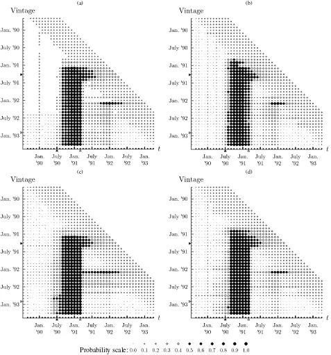
Figures5and6 display the real-time posterior probabilities Pr[s1,t =1|YT−1] obtained using the vintages before, during,
and after the recessions in 1990–1991 and 2001, respectively. In these graphs, the horizontal axis displays time, t, and the vertical axis dieplays the release date of the vintage, T−1. Thus each row in these graphs displays the values of the poste-rior probabilities of a recession over time based on the vintage released at the end of the month as indicated on the vertical axis. Recession probability Pr[s1,t =1|YT−1] values of≥0.5
are represented by black dots; values < 0.5, as white dots. The size of the dots indicates the actual value of the recession probability. If for one particular vintage, the dots change from white to black in a certain calender month and remain black consistently thereafter, then this month is considered a business cycle peak. A change from black to white similarly indicates a trough. Conversely, looking across rows reveals how this as-sessment changes across data releases. If the posterior proba-bilities based on some vintage show a particular recession for
the first time and this recession persists in the results thereafter, then the release date of the first vintage is identified as the de-tection date of the recession.
For the period before, during, and after the July 1990–March 1991 recession, all models produce a fairly stable pattern of re-cession probabilities from the July 1991 vintage onward. Con-sistent with the results for the July 2007 vintage shown in Figure4, the signals of the synchronous and the nonsynchro-nous common cycle specifications are less clear than those of the other two specifications, in the sense that no sharp regime switches are seen. It would be particularly difficult to date the trough using the synchronous cycle specification. When using the nonsynchronous cycle specification, we would be unsure about the date of the peak. Based on the asymmetric nonsyn-chronous common cycle specification, we would date the peak at September 1990, two months later than the NBER’s peak date. Our estimate of the trough exactly matches the NBER’s date, however. In terms of the speed of detection of the busi-ness cycle peak, we observe a first string of recession probabil-ities>0.5 for the data release of December 1990, four months before the NBER’s announcement of the peak. The indepen-dent cycles and the nonsynchronous common cycle specifica-tions detect the recession two months later, in February 1991. As early as June 1991, our model indicates that a trough had occurred in March. The NBER announced the end of this re-cession in December 1992, nearly one and a half years after the model’s time of detection.
The results for the March–November 2001 recession shown in Figure6demonstrate the advantage of the asymmetric non-synchronous common cycle specification more convincingly. The most prominent feature of the recession probabilities in these graphs is the false signal given by the other three cycle specifications for the period September 2002–September 2003. The increase in recession probability during this period is much less for the asymmetric nonsynchronous common cycle speci-fication. For the 2001 recession itself, the two nonsynchronous common cycle models provide a much earlier and clearer sig-nal of the peak than the independent cycles and synchronous common cycle specifications. For both nonsynchronous com-mon cycle specifications, the recession probabilities increase for the first time with the July 2001 vintage. Again the models signal this recession considerably earlier than the NBER, whose announcement of the peak came four months later, in Novem-ber 2001. The model’s timeliness is even more pronounced for the subsequent trough, which we first detect when using the March 2002 data vintage, whereas the corresponding NBER an-nouncement came only in July 2003. Concerning the dating of the turning points, based on the asymmetric lead/lag specifica-tion, we would have concluded that the recession started in Jan-uary 2001, two months earlier than the NBER’s date. The end of the recession also occurs a few months after the official trough in November 2001.
5.2 Forecasting Results
We conclude our analysis by evaluating the (relative) accu-racy of real-timeh-month-ahead forecasts of the business cycle regime and of CCI growth rates forh=1,2, . . . ,12. To
(a) (b)
(c) (d)
Probability scale:
Figure 5. In-sample estimates and out-of-sample predictions of recession probabilities in a rolling horizon: the July 1990 to March 1991 recession. The graphs present the estimated and predicted recession probabilities in a rolling horizon, where at every point in time the latest data vintage is used to compute in-sample estimates for the past and out-of-sample predictions for the next 12 months ahead. On the vertical axes, the announcement date of the July 1990 business cycle peak (April 25, 1991) and the March 1991 business cycle trough (December 22, 1992) are marked by the black and white pointers, respectively. Likewise, on the horizontal axes, the pointers mark the dates of the peak and trough itself.
ate the latter forecasts, we use the mean squared forecast error (MSFE),
MSFE(h)= 1
T2−h−T1
T2−h
t=T1−1
y1,t+h− ˆy1,t|t+h
2
, (23)
whereT1andT2correspond to the first and last data vintages considered (January 1989 and July 2007),yˆ1,t|t+h denotes the
h-step-ahead forecast made at time t+1, and y1,t+h is the
monthly CCI growth rate resulting from the release of the se-ries in July 2007. To measure the deviation between the regime variables1,tand the recessions according to the NBER turning
points, we use the turning point forecast error (TPFE),
TPFE(h)= 1
T2−h−T1
T2−h
t=T1−1
NBERt+h− ˆs1,t|t+h2
forh=1, . . . ,12, (24)
(a) (b)
(c) (d)
Probability scale:
Figure 6. In-sample estimates and out-of-sample predictions of recession probabilities in a rolling horizon: the March to November 2001 recession. The graphs present the estimated and predicted recession probabilities in a rolling horizon, where at every point in time the latest data vintage is used to compute in-sample estimates for the past and out-of-sample predictions for the next 12 months ahead. On the vertical axes, the announcement date of the March 2001 business cycle peak (November 26, 2001) and the November 2001 business cycle trough (July 17, 2003) are marked by the black and white pointers, respectively. Likewise, on the horizontal axes, the pointers mark the dates of the peak and trough itself.
where ˆs1,t|t+h denotes the h-step-ahead forecast of the state
variable made at timet+1 and NBERt+his a binary variable
that equals 1 if, according to the NBER turning points, the econ-omy is in recession at timet+h. An alternative approach to forecasting turning points based directly on the NBER turning points or a different sequence of peaks and troughs is the Qual VAR model ofDueker (2005). Extending that model to explic-itly incorporate asymmetric lead times at peaks and troughs is
an interesting challenge but is beyond the scope of the present work.
To facilitate the forecast comparison, we take the most general model specification—the asymmetric nonsynchronous common cycle model—as a reference point. The first panel of Figure7displays ratios of the TPFE(h) forh-step-ahead fore-casts of probability of recession obtained from the MS-VAR models with independent cycles, with a synchronous common
(a) (b)
Figure 7. Regime and CCI growth rate prediction error ratios. The graphs present forecasting error ratios obtained from the MS-VAR models with independent cycles, a synchronous common cycle, and a symmetric nonsynchronous common cycle relative to the asymmetric nonsynchro-nous common cycle model. (a) The TPFE(h) for forecasts of the recession probabilities, whereh=1,2, . . . ,12. (b) The MSFE(h) for forecasts of CCI growth.
cycle and a symmetric nonsynchronous common cycle relative to the asymmetric nonsynchronous common cycle model. We see that the asymmetric model outperforms the other models in forecasting turning points as all ratios exceed unity. The im-provement in forecast accuracy is especially large for short hori-zons, up to 30%. For horizons longer than 6 months, the dif-ferences are relatively small, especially with the models with independent cycles and a synchronous common cycle.
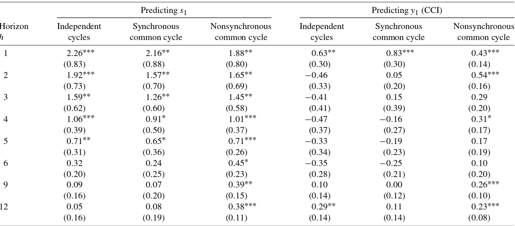
We test whether the differences in TPFEs are statistically sig-nificant using the Diebold and Mariano (1995) test of equal predictive accuracy. The results in the left panel of Table 3
for forecast horizons h=1, 2, 3, 6, 9, and 12 months con-firm the graphical evidence given in Figure 7. In particular,
the asymmetric nonsynchronous common cycle model pro-vides significantly more accurate forecasts than the other three variants for horizons up to five months. For longer horizons, only the symmetric nonsynchronous cycle specification is still significantly worse than our asymmetric lead time specifica-tion.
The second panel of Figure 7 displays the ratios of the
MSFE(h) for h=1, . . . ,12 for CCI growth forecasts for the same three models relative to the asymmetric nonsynchronous cycle model. Here the results are more mixed. For forecast hori-zons of 1 month and longer than 7 months, the novel cycle specification outperforms the other models. TheDiebold and Mariano (1995)test results displayed in the right panel of
Ta-Table 3. Testing equal predictive accuracy
Predictings1 Predictingy1(CCI)
Horizon Independent Synchronous Nonsynchronous Independent Synchronous Nonsynchronous
h cycles common cycle common cycle cycles common cycle common cycle
1 2.26∗∗∗ 2.16∗∗ 1.88∗∗ 0.63∗∗ 0.83∗∗∗ 0.43∗∗∗
(0.83) (0.88) (0.80) (0.30) (0.30) (0.14)
2 1.92∗∗∗ 1.57∗∗ 1.65∗∗ −0.46 0.05 0.54∗∗∗
(0.73) (0.70) (0.69) (0.33) (0.20) (0.16)
3 1.59∗∗ 1.26∗∗ 1.45∗∗ −0.41 0.15 0.29
(0.62) (0.60) (0.58) (0.41) (0.39) (0.20)
4 1.06∗∗∗ 0.91∗ 1.01∗∗∗ −0.47 −0.16 0.31∗
(0.39) (0.50) (0.37) (0.37) (0.27) (0.17)
5 0.71∗∗ 0.65∗ 0.71∗∗∗ −0.33 −0.19 0.17
(0.31) (0.36) (0.26) (0.34) (0.23) (0.19)
6 0.32 0.24 0.45∗ −0.35 −0.25 0.10
(0.20) (0.25) (0.23) (0.28) (0.21) (0.20)
9 0.09 0.07 0.39∗∗ 0.10 0.00 0.26∗∗∗
(0.16) (0.20) (0.15) (0.14) (0.12) (0.10)
12 0.05 0.08 0.38∗∗∗ 0.29∗∗ 0.11 0.23∗∗∗
(0.16) (0.19) (0.11) (0.14) (0.14) (0.08)
NOTE: The left panel of the table shows the difference between the TPFE(h) defined in (24) of the indicated cycle specification and the TPFE(h) of the asymmetric nonsynchronous common cycle specification. The right panel shows corresponding differences for the MSFE(h) defined by (23). Heteroscedasticity and autocorrelation consistent (HAC) standard errors are in parentheses. All numbers are×100. The superscripts∗∗∗,∗∗, and∗indicate significance at the 1%, 5%, and 10% level, respectively, of the Diebold–Mariano (1995) statistic for testing the null hypothesis that the difference in TPFE(h) or MSFE(h) is equal to 0.
ble3 indicate significant differents MSFEs for 1-month-ahead forecasts. This also holds for 12-month-ahead forecasts for the models with independent cycles and a symmetric nonsynchro-nous common cycle. At intermediate horizons, the indepen-dent cycle specification provides the most accurate forecasts, although the gain relative to the asymmetric nonsynchronous common cycle specification is not statistically significant; see Table3.
In summary, our model produces sharper and more accurate turning point estimates, particularly for business cycle peaks. Concerning the speed of detection, our model is advantageous, especially in detecting business cycle troughs. For the last two recessions, it detected troughs more than 1 year ahead of the NBER’s announcements. The model also provides more ac-curate forecasts than the other models, especially for turning points.
6. CONCLUSIONS
In this article we have presented a formal statistical approach to investigate whether the lead time of leading indicator vari-ables differs at business cycle peaks and troughs. We have pro-posed a novel MS-VAR model in which economic growth and leading indicators share a common Markov process determin-ing the state but with different lead times at switches between the different regimes for this purpose. An empirical applica-tion involving The Conference Board’s monthly CCI and CLI demonstrates the usefulness of our new model specification. For the period of January 1959–June 2007, we found that on av-erage the CLI led CCI by nearly 1 year at peaks but by only 1 quarter at troughs. Thus, in terms of timeliness, the CLI was most useful for signaling oncoming recessions. In addition, in a real-time business cycle dating and forecasting exercise for the vintages in the period of January 1989–July 2007, we found that allowing for asymmetric lead times led to more timely and precise identification of peaks and troughs for the 1990–1991 and 2001 recessions, as well as more accurate out-of-sample turning point forecasts. whereIm denotes the (m×m) identity matrix. This is a
re-gression model with parameter Ŵ0 and an error term with
unit variance. Thus the full conditional posterior distribu-tion of Ŵ0 is normal with mean (X′X)−1X′Z and
covari-e.g.,Zellner 1971, chapter III). The prior restriction for identi-fication can be easily incorporated by sampling from truncated normal distributions.
This is a regression model with parameterŴ1and an error term with unit variance. The full conditional posterior distribution ofŴ1is normal with mean(X′X)−1X′Zand covariance matrix
striction for identification can be easily incorporated by sam-pling from truncated normal distributions.
A.3 Sampling of
To sample, we note that (13) is a multivariate regression model with regression parameters i for i=1, . . . ,k. Define
Zt=(Yt−Ŵ0−Ŵ1⊙St)andZj=(Zk−j+1, . . . ,ZT−j)′. This
multivariate regression model can be written as
Z=X+e, (A.3)
T ET)′. Thus the full conditional posterior distribution of
is a matric variate normal distribution with mean(X′X)−1X′Z
and covariance matrixIm⊗(X′X)−1, seeZellner(1971,
chap-ter VIII). Here⊗denotes the Kronecker product. To sample in the case with zero restrictions on the elements of, we rewrite (A.3) in a univariate linear regression model with regression parameter vec()using the vec operator, that is,
vec(Z)=vec(I⊗X)vec()+vec(e), (A.4)
allowing us to sample the nonzero elements of vec() from a normal distribution with mean (X˜′X˜)−1(X˜′vec(Z)) and
co-variance matrix (X˜′X˜)−1, where X˜ contains the columns
of vec(I ⊗X) corresponding to the nonzero elements of
vec().
A.4 Sampling of0and1
It is easy to see from the conditional likelihood (15) and the prior specification (21) that the full conditional posterior of den-sity0and1is proportional to
where A\ B denotes the set A excluding the elements in setB. Thus the covariance matrixes0 and1 can be sam-pled from inverted Wishart distributions with scale parame-ters(τ−1
From the conditional likelihood function (15), it follows that the full conditional posterior densities of the transition parame-ters are given by
whereNi,j again denotes the number of transitions from state
ito statej. This implies that the transition probabilities can be sampled from Beta distributions with parametersN0,0+1 & N0,1+1, andN1,1+1 &N1,0+1. In the case with separate
state variables for the two series, we can sample both transition probabilities separately.
A.6 Sampling ofτ
The full conditional posterior density ofτ is given by
f(τ|sT T−ν]we can easily sample from its full conditional posterior distribution.
A.7 Sampling ofκ
If our model contains nonsynchronous cycles in both series, then we must sample one or twoκ parameters. Because theκ
parameters are discrete, we can compute the value of the pos-terior distribution forκj∈ {−cj, . . . ,cj}and scale these values
such that they add up to 1. We can now easily sample a value for κ. Note that we can sample κ1 andκ2 at once from their joint full conditional distribution.
A.8 Sampling of the States
To sample the states, we need the full conditional poste-rior density ofs1,t, denoted byf(s1,t|s1−t,θ,YT),t=1, . . . ,T,
where s−t
1 =s
T
1 \ {s1,t}. Because s1,t follows a first-order Markov process, it is easily seen that
f(s1,t|s1−t)∝f(s1,t|s1,t−1)f(s1,t+1|s1,t) (A.9)
due to the Markov property. Thus the full conditional distribu-tion ofs1,tis given by be obtained by summing over the two possible values ofs1,t.
At timet=T, the termf(s1,T+1|s1,T,θ)drops out. The firstk
states can be sampled from the full conditional distribution
f(s1,t|s−1t,θ,YT)∝f(s1,t|s1,t−1,θ)f(s1,t+1|s1,t,θ)
Sampling of the state variables can be done as follows. Take the most recent value ofsT
1 and sample the states backward in time, one after another, starting withs1,T. After each step,
re-place thetth element ofsT
1 by its most recent draw.
ACKNOWLEDGMENTS
We thank the participants of the conference on Nonlinear-ity and the Business Cycle at Washington UniversNonlinear-ity in August 2004, the Econometric Society European Meeting in Vienna in August 2006, the 17th (EC)2Meeting in Rotterdam in De-cember 2006, the conference on Growth and Business Cycles in Theory and Practice in Manchester in July 2007, and semi-nars at HEC (Montréal) and CREATES (Århus), as well as the associate editor and two anonymous referees for their helpful comments and suggestions. Any remaining errors are our own. We also thank Ataman Ozyildirim at The Conference Board for providing the real-time CLI and CCI data. Please check our websitehttp:// www.businesscycles.usfor up-to-date forecasts.
[Received March 2007. Revised January 2008.]
REFERENCES
Albert, J. H., and Chib, S. (1993), “Bayes Inference via Gibbs Sampling of Autoregressive Time Series Subject to Markov Mean and Variance Shifts,”
Journal of Business & Economic Statistics, 11, 1–15.
Boldin, M. D. (1996), “A Check on the Robustness of Hamilton’s Markov Switching Approach to the Economic Analysis of Business Cycles,”Studies in Nonlinear Dynamics and Econometrics, 1, 35–46.
Burns, A. F., and Mitchell, W. C. (1946),Measuring Business Cycles, New York: National Bureau of Economic Research.
Camacho, M., and Perez-Quiros, G. (2002), “This Is What the Leading Indica-tors Lead,”Journal of Applied Econometrics, 17, 61–80.
Chauvet, M. (1998), “An Econometric Characterization of Business Cycle Dy-namics With Factor Structure and Regime Switching,”International Eco-nomic Review, 39, 969–996.
Chauvet, M., and Hamilton, J. D. (2006), “Dating Business Cycle Turning Points,” inNonlinear Time Series Analysis of Business Cycles, eds. C. Mi-las, P. Rothman, and D. van Dijk, Boston: Elsevier, pp. 1–54.
Chauvet, M., and Piger, J. (2008), “A Comparison of the Real-Time Perfor-mance of Business Cycle Dating Methods,”Journal of Business & Eco-nomic Statistics, 26, 42–49.