Full Terms & Conditions of access and use can be found at
http://www.tandfonline.com/action/journalInformation?journalCode=ubes20
Download by: [Universitas Maritim Raja Ali Haji] Date: 12 January 2016, At: 00:21
Journal of Business & Economic Statistics
ISSN: 0735-0015 (Print) 1537-2707 (Online) Journal homepage: http://www.tandfonline.com/loi/ubes20
Testing for Serial Correlation: Generalized
Andrews–Ploberger Tests
John C. Nankervis & N. E. Savin
To cite this article: John C. Nankervis & N. E. Savin (2010) Testing for Serial Correlation:
Generalized Andrews–Ploberger Tests, Journal of Business & Economic Statistics, 28:2, 246-255, DOI: 10.1198/jbes.2009.08115
To link to this article: http://dx.doi.org/10.1198/jbes.2009.08115
Published online: 01 Jan 2012.
Submit your article to this journal
Article views: 95
View related articles
Testing for Serial Correlation: Generalized
Andrews–Ploberger Tests
John C. N
ANKERVISEssex Finance Centre, Essex Business School, University of Essex, Colchester, CO4 3SQ, U.K.
N. E. S
AVINDepartment of Economics, University of Iowa, Iowa City, IA 52242 (gene-savin@uiowa.edu)
This paper considers testing the null hypothesis that a times series is uncorrelated when the time series is uncorrelated but statistically dependent. This case is of interest in economic and finance applications. The GARCH(1,1)model is a leading example of a model that generates serially uncorrelated but statistically dependent data. The tests of serial correlation introduced by Andrews and Ploberger (1996, hereafter AP) are generalized for the purpose of testing the null. The rationale for generalizing the AP tests is that they have attractive properties for cases for which they were originally designed: they are consistent against all nonwhite-noise alternatives and have good all-round power against nonseasonal alternatives compared to several widely used tests in the literature. These properties are inherited by the generalized AP tests.
KEY WORDS: Autoregressive moving average model; Lagrange multiplier test; Nonstandard testing; Statistically dependent time series; Uncorrelatedness.
1. INTRODUCTION
As noted by Hong and Lee (2003), there has been growing in-terest in developing consistent tests for serial correlation of un-known form; examples include Andrews and Ploberger (1996, hereafter AP), Hong (1996), Chen and Deo (2004) in estimated regression residuals, Durlauf (1991), and Deo (2000) in the observed raw data. The tests assume independently and iden-tically distributed regression errors under the null except for Deo (2000), which generalizes Durlauf (1991) to allow for a re-strictive form of conditional heteroscedasticity. This paper con-siders testing the null that a times series is uncorrelated when the time series is uncorrelated but statistically dependent. For a more extensive literature review, see Francq, Roy, and Zakoian (2005).
The case of uncorrelated dependent time series is of interest in economic and financial applications because many problems such as financial (non-) predictability are related to a martingale difference sequence (MDS) hypothesis after demeaning, which implies serial uncorrelatedness but not serial independence. The GARCH(1,1)model is a leading example of a model that gen-erates serially uncorrelated but statistically dependent data. The rationale for generalizing the AP tests is that they are consistent against all nonwhite-noise alternatives and have good all-round power against nonseasonal alternatives when compared to sev-eral tests in the literature, including the Box–Pierce (1970, here-after BP) tests. The generalized AP tests inherit the properties of the AP tests in power comparisons. In our simulation ex-periments, the generalized AP tests typically have substantially better power than the generalized BP (Lobato, Nankervis, and Savin 2002) tests against nonseasonal alternatives and power equal to or better than the Deo (2000) test.
AP introduced tests of serial correlation designed for the case where the time series is generated by ARMA(1,1) mod-els under the alternative. As they noted, it is natural to consider tests of this sort because ARMA(1,1)models provide parsimo-nious representations of a broad class of stationary time series.
ARMA(1,1)models for financial returns series follow from the mean-reversion models of Poterba and Summers (1988) and the price-trend models of Taylor (2005). However, testing for serial correlation generated by an ARMA(1,1)model is a nonstan-dard testing problem because the ARMA(1,1)model reduces to a white-noise model whenever the AR and MA coefficients are equal. The testing problem is one in which a nuisance para-meter is present only under the alternative hypothesis. For the problem addressed by AP, the standard likelihood ratio (LR) statistic does not possess its usual asymptotic chi-squared dis-tribution or its usual asymptotic optimality properties. It is also possible that an ARMA(1,1)generates white noise when the AR and MA coefficients are not equal, as is the case for the all-pass filter model; see Andrews, Davis, and Breidt (2006).
The LR test has the attractive feature of being consistent against all forms of serial correlation (Potscher1990). AP show that this feature also holds for tests introduced into the lit-erature by Andrews and Ploberger (1994, 1995), namely, the sup Lagrange Multiplier (LM) and average exponential LM and LR tests. AP establish the asymptotic null distribution for the LR, sup LM, and average exponential test statistics un-der the assumption that the generating process is a condition-ally homoscedastic martingale difference sequence (MDS). The asymptotic critical values for these tests were calculated by simulation. In Monte Carlo power experiments, AP compared the finite-sample powers of the LR, sup LM, average expo-nential, BP, and other tests. The alternatives include Gaussian ARMA(1,1)models. Against this class of alternatives, the LR test was found to have very good all-around power properties for nonseasonal alternative models, especially compared to BP tests.
For serially uncorrelated but statistically dependent time se-ries, the true levels of the LR, sup LM, and average exponential
© 2010American Statistical Association Journal of Business & Economic Statistics
April 2010, Vol. 28, No. 2 DOI:10.1198/jbes.2009.08115
246
tests can differ substantially from the nominal levels when the tests use the asymptotic critical values calculated by AP. This paper generalizes a subset of the tests considered by AP so that they have the correct level asymptotically when the time series is serially uncorrelated but statistically dependent. The subset consists of LM-based tests, namely the sup LM test and the av-erage exponential LM tests. The generalization is obtained by using the true asymptotic covariance matrix of the sample auto-correlations, or a consistent estimator. The same approach has been used by Lobato, Nankervis, and Savin (2002) to generalize the BP tests to settings where the time series is serially uncor-related but statistically dependent. The asymptotic critical val-ues reported by AP remain valid for the generalized LM-based tests.
The finite-sample levels of the generalized LM-based tests with asymptotic critical values are assessed by simulation. In Monte Carlo power experiments, these tests are compared to generalized BP tests and the Deo (2000) test. The generalized AP tests typically have better level-corrected power against nonseasonal alternatives. Hence, generalized AP tests can be recommended for use in economic and finance applications. The paper reports the results of an empirical application to stock return indexes.
2. ARMA(1, 1) MODEL AND TEST STATISTICS
This section reviews the model, hypothesis, and test statistics considered by AP.
isB. They assume thatandBare such that the absolute value of the autoregressive coefficient|π+β|<1, is closed and Bcontains a neighborhood of zero. The former condition rules out unit root and explosive behavior of{Yt:t=1, . . . ,T}.
The null hypothesis is that{Yt:t=1, . . . ,T}is white noise,
and the alternative is that{Yt:t=1, . . . ,T}is serially
corre-lated. These hypotheses are given by
H0:β=0 and H1:β=0. (2)
Whenβ=0, the model (1) reduces toYt=εt, and the
parame-terπ is no longer present. The testing problem is nonstandard becauseπis not identified when the null hypothesis is true.
Let LRT(π )denote the standard LR statistic for testingH0
versusH1whenπis known under the alternative. Then the LR
statistic for the unknownπ is
LR=sup
AP proved that an asymptotically equivalent test statistic to the LR statistic (under the null and local alternatives) is the sup LM statistic
The LR and sup LM tests are shown to satisfy an asymptotic admissibility property, and as a consequence, beat any given test in terms of weighted average power against alternatives that are local to, but sufficiently distant from the null; for details, see p. 1333 of AP.
Andrews and Ploberger (1994) introduced average expo-nential tests. These tests are asymptotically optimal in the sense that they minimize weighted average power for a spe-cific weight function. The weight functions for the parameter
β are mean zero normal densities with variances proportional to a scalarc>0. The weight functionJ for the parameterπ
is chosen by the investigator. For the simulation results in AP, the function is taken to be uniform on, and similarly in this article. For each c∈(0,∞), the average exponential LM test
measure on. The average exponential LR test statistic, Exp-LRcT, is defined analogously with LMT(π )being replaced by
LRT(π ). The limiting average exponential LM test statistics as
c→0 andc→ ∞are given by
Andrews and Ploberger (1994) show that the average exponen-tial tests have asymptotic local power optimality properties.
248 Journal of Business & Economic Statistics, April 2010
3. ASYMPTOTIC AND FINITE–SAMPLE NULL DISTRIBUTIONS OF AP TEST STATISTICS
AP established the asymptotic null distribution of the test sta-tistics previously introduced. This section reviews the asymp-totic theory.
The asymptotic null distributions of the test statistics are es-tablished by showing that the sequences of stochastic processes {LRT(·):T≥1}and{LMT(·):T≥1}indexed byπ∈
con-verge weakly to a stochastic processG(·)and then by applying the continuous mapping theorem. Let⇒denote weak conver-gence of a sequence of stochastic processes and let→d denote converge in distribution of a sequence of random variables. Let {Zi:i≥0}be a sequence of iid N(0,1)random variables.
De-fine
G(π )=(1−π2)
∞
i=0 πiZi
2
forπ∈. (8)
The following theorem is proved by AP under a variety of as-sumptions.
Theorem 1.
a. LMT(·)⇒G(·),
b. supπ∈LMT(π ) d
→supπ∈G(π ), c. Exp-LM0T →d G(π )dJ(π ), d. Exp-LM∞T
d
→lnexp(12G(π ))dJ(π ), and e. parts (a)–(d) hold with LM replaced by LR.
Theorem1holds for time series where the asymptotic covari-ance matrix of the firstT−1 of the sample autocorrelations is equal to the identity matrix. A time series generated by a condi-tional homoscedastic martingale difference sequence is an ex-ample where the asymptotic covariance matrix of the sex-ample autocorrelations is the identity matrix. On the other hand, The-orem1does not hold for many models used in economics and finance, for example, a GARCH(1,1)with normal innovations. The implications of the identity matrix condition for testingH0
are explored in the next section.
From Theorem 1, the LR, sup LM, and average exponen-tial LR and LM tests are asymptotically pivotal, that is, the asymptotic distribution does not depend on any unknown pa-rameters. Hence, the asymptotic critical values for the tests can be simulated by truncating the series∞i=0πiZiat a large value
Tr. AP report simulated critical values of the tests in their
ta-ble 1. The critical values are based on the parameter space
= {0,±0.01, . . . ,±0.79,±0.80},Tr=50 and 40,000
repe-titions. They also calculate finite-sample critical values for the tests.
The LR, sup LM, and average exponential LR and LM tests are shown by AP to be consistent against all deviations from the null hypothesis of white noise within a class of weakly sta-tionary strong mixing sequences of random variables. This con-sistency property illustrates the robust power properties of the tests.
The tests introduced by AP can also be used to test whether regression errors are serially correlated. The tests are con-structed using the residuals{ ˆYt:t≤T}rather than the random
variables{Yt:t≤T};see AP for details. Provided that the
re-gressors are exogenous, the resulting LR, sup LM, and average exponential LR and LM test statistics have the same asymptotic
distributions as when the actual errors are used to construct the statistics. Thus, the asymptotic critical values previously cal-culated by AP are applicable. However, the tests are not valid when applied to the residuals of a dynamic regression model.
4. GENERALIZATION OF LM BASED TESTS
In this section, the LM-based tests considered by AP are gen-eralized such that the tests have the correct asymptotic level under the null when the asymptotic covariance matrix of the sample autocorrelations is not the identity matrix. The asymp-totic distributions of the generalized AP test statistics are based on a central limit theorem for the sample autocorrelations and a consistent estimator of the asymptotic covariance matrix.
We begin with a review of the asymptotic distribution theory of the sample autocorrelations when{Yt:t=1,2, . . .}is a
co-variance stationary sequence of statistically dependent but un-correlated random variables with mean zero (or allow for mean
μ, as we do below). Define the lag-j autocovariance by γj=
E(YtYt+j)and the lag-jautocorrelation byρj=γj/γ0. The
vari-ance and lag-jautocovariance are given byγ0ˆ =Tt=1(Yt)2/T
andγˆj=Tt=−1j(YtYt+j)/T. We assume thatYtis a weak
depen-dent process for which the vector of sample autocovariances
γ=(γ1, γ2, . . . , γK)′ satisfies the following central limit
theo-rem: √T(γˆ −γ )′→d N(0,C), whereC (assumed to be finite and positive definite) is 2π times the spectral density matrix at zero frequency of the vector with elementsYtYt−j.
A straightforward application of the delta method leads to a central limit theorem for the sample autocorrelations: Under general weak dependence conditions,
√
Tr=√T(r1,r2, . . . ,rK)′ d
→N(0,V), (9)
whererj= ˆγj/γˆ0and theijth element ofV is given in Lobato,
Nankervis, and Savin (2002, p. 732) and Romano and Thombs (1996). A variety of weak dependence conditions are reviewed in Lobato, Nankervis, and Savin (2002). Using the idea of near epoch dependence (NED), De Jong and Davidson (2000) show that the preceding central limit theorem forγˆ holds under the following assumption:
Assumption 1. LetYtbe a covariance stationary process that
satisfiesE|Yt|s<∞for somes>4 and alltand is L2-NED of
size –1/2 on a processUtwhereUtis anα-mixing sequence of
size−s/(s−4).
Davidson (2000) has proved that many nonlinear time series models satisfy the NED assumption.
Next consider testing the null hypothesisH0(K):ρ=(ρ1, . . . , ρK)′ =0 against the alternative ρ =0. Suppose V is
known. Then a test can be based on the test statistic
BPK(V)=Tr′V−1r, (10)
where the statistic is asymptotically chi-square distributed with K degrees of freedom whenH0(K) is true. In practice, V is unknown. In the standard BP statistic,V is replaced byI, the identity matrix. IfVis not equal to the identity, the standard BP test can produce misleading inferences.
Under the null,V simplifies toV0= [(γ0)−2C0] whereC0
has as itsijth element
c0ij=
Nankervis, and Savin (2002) use this simplification to construct a generalized BP test statistic. This test statistic is
BPK(Vˆ0)=Tr′(Vˆ0)−1r, (12)
whereVˆ0is a consistent estimator ofV0underH0(K). A
con-sistent estimator can be obtained by usingγ0ˆ to estimateγ0and a consistent nonparametric estimator ofC0.
Our generalization of the LM-based tests exploits the fact that the LM test statistic is a function of sample autocorrela-tions. Rewriting the LMT(π )statistic in (5) gives
where theith sample autocorrelation in (13) is
ri=
ried out using the asymptotic critical values calculated by AP. IfV=I, the true levels of the tests with AP asymptotic critical values can differ substantially from the nominal levels in finite samples and asymptotically.
The level distortion of the LM-based tests whenV=I can be corrected asymptotically by using√TLrin place of√Tr, whereV−1=L′L. Our proposed generalization is to replaceV
byV0and consistently estimateV0byVˆ0. The generalized tests we consider are
A brief sketch of a proof that the generalized AP tests have the same limiting distribution as the AP tests is the following. In the AP case where Var(√Tr)=I, we have that
of correlated asymptotically standard normal variables,
T(1−πj2)pj′r. In the case where Var(√Tr)=Vwe have that
T(1−π2)p′Lˆ0r d
→N(0,1),
and that the asymptotic correlation between
same functions of asymptotically standard normal variables with identical asymptotic correlations.
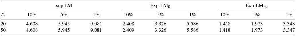
The asymptotic critical values reported by AP remain valid for our generalization of the LM-based tests. We use critical values based onTr=20, whereas AP useTr=50. We have set,
as AP did, max|π| =0.8. UsingTr =20 rather than 50 has a
negligible effect on the 1%, 5%, and 10% asymptotic critical values through terms (1−π2×Tr−1). This is seen in Table1 where we report the asymptotic critical values for the three test statistics for = {0,±0.01, . . . ,±0.79,±0.80},Tr=20 and
Tr=50, using 150 million replications.
The generalized versions of BP and LM-based tests require a consistent estimator of V0. We use the VARHAC estima-tion procedure proposed by den Haan and Levin (1997). The consistency of the VARHAC estimator is proved by den Haan and Levin (1998) under very general conditions. They demon-strate that, in many cases, the VARHAC estimator achieves
Table 1. Asymptotic critical values
sup LM Exp-LM0 Exp-LM∞
Tr 10% 5% 1% 10% 5% 1% 10% 5% 1%
20 4.608 5.945 9.081 2.408 3.326 5.586 1.418 1.973 3.348
50 4.608 5.945 9.081 2.409 3.326 5.586 1.418 1.973 3.347
NOTE: Critical values obtained by setting= {0,±0.01, . . . ,±0.79,±0.80}. The number of replications is 150 million.
250 Journal of Business & Economic Statistics, April 2010
a faster convergence rate than kernel-based methods. Francq, Roy, and Zakoian (2005, p. 539) also prove the consistency of the VARHAC estimator. Their proof uses the existence of the eighth moment ofYtand a mixing condition.
The VARHAC procedure uses a vector autoregressive (VAR) estimator of the covariance matrix where the order of equa-tions in the VAR is automatically selected. To present the ex-plicit formula for the VARHAC estimator of C0, let wˆit =
(Yt− ¯Y)(Yt−i− ¯Y),wˆt=(wˆ1t, . . . ,wˆTr,t)′, and letS¯be the max-imum lag order chosen for the VAR. For consistency, den Haan and Levin (1998) also require that the maximum lag grows at rateT1/3. The estimated residuals from the VAR regressions are
ˆ
where Aˆs are the matrices of estimated coefficients from the
VAR, and the estimated innovation covariance matrix is
Then the VARHAC estimator ofC0is
ˆ
We report results for the VAR with the AIC (Akaike1973) and the SBC (Schwarz1978) criteria. The resulting estimators are denoted byVˆ(AIC)andVˆ(SBC). The maximum lag length is 3, 4, 5, and 8 for sample sizesT=200,500,1,000, and 5,000, and, for any equation in the VAR, the same lag length is used for each element of the vector process. To mitigate the effect of oc-casional extreme estimates we used the procedure of Andrews and Monahan (1992), and set the minimum singular values of the inverse of the recoloring matrix,I−Ss¯=1Aˆ′s,to be 0.005.
The form of theV0matrix is simplified when the time series is a martingale difference sequence. For a MDS process, the only possible nonzero elements of C0 are terms of the form E(Yt−μ)2(Yt−i−μ)(Yt−j−μ). In (11) these occur atd=0.
Guo and Phillips (1998) have developed a version of the BP test for the MDS case. This special form ofV0matrix can also be used in constructing a generalization of the LM-based tests for general MDS processes.
For certain MDS processes, such as Gaussian GARCH processes,V0is diagonal, with thejth diagonal element equal to(γ (0))−2E(Yt−μ)2(Yt−j−μ)2. Generalizations of the
LM-based tests can be constructed for the diagonal case. The BP test for the diagonal case has been repeatedly reinvented in the literature; see, for example, Taylor (1984), Diebold (1987), Lo and MacKinlay (1989), Lobato, Nankervis, and Savin (2001), and also Deo (2000).
We denote the estimator ofV0in the general MDS case by VGP. A consistent estimator of theijth element ofVGPis
ˆ
The diagonalV0matrix is denoted byV∗. A consistent estima-tor of thejth diagonal element ofV∗is
As noted earlier, AP show that their tests apply to residuals from regressions with exogenous regressors (assumptions 4 and 5 in AP). The same holds for the generalized tests. The reason these assumptions rule out an extension to dynamic regression mod-els is because they require that the conditional mean of the un-observed errors is zero given past values of the errors and past andfuturevalues of the regressors.
5. MONTE CARLO COMPARISONS
This section considers the true levels of the LM-based tests, the BP tests, and the Deo (2000) test when the tests use asymp-totic critical values. The LM-based tests are the sup LM, Exp-LM0, and Exp-LM∞ tests. The finite sample level-corrected
powers of these tests and the other tests are compared. The BP tests are included because they are widely employed in the economics and finance literature and the Deo (2000) test is in-cluded because it is consistent against all nonwhite-noise alter-natives whenV is diagonal in the MDS case, a property not shared by the BP tests.
The model we consider in the level experiments is the loca-tion model with serially uncorrelated but dependent errors,
Yt=μ+εt fort=1,2, . . . ,T, (18)
where V =I. The models used for the errors εt in the
ex-periments include two MDS processes and two non-MDS processes.
The two MDS models for the errors are variants of the GARCH model of Bollerslev (1986), namely, Gaussian GARCH(1,1) and the exponential GARCH(1,1) or EGARCH(1,1). Both models are described in Campbell, Lo, and MacKinlay (1997).
GARCH(1,1).εt=Zt·σt, where{Zt}is an iid N(0,1)
se-quence andσt2=ω+α0ε2t−1+β0σt2−1. The constantsα0 and β0are such thatα0+β0<1. This condition is needed so that
Ytis covariance stationary. He and Teräsvirta (1999) show that
the unconditional 2mth moment ofYt for GARCH(1,1)
mod-els ofYt exists if and only ifE(α0Zt2+β0)m<1. We setω=
0.001, α0=0.08, andβ0=0.89. With this parameter setting,
the He and Teräsvirta conditions for the existence of the fourth and eighth moments ofYt are satisfied. For this process,γ0=
E(Yt−μ)2=0.033,E(Yt−μ)3/γ03/2=0,E(Yt−μ)4/γ04=
3.83, andV is diagonal. We note that our results are invariant to the value ofω. Estimates from stock return data suggest that
α0+β0is close to one withβ0also close to one; for example,
see Bera and Higgins (1997).
EGARCH(1,1). εt=Zt ·σt, where {Zt} is an iid N(0,1)
sequence and where ln(σt2)=ω+ψ|Zt−1| +α0Zt−1+β0×
ln(σt2−1). We setω=0.01, ψ=0.5, α0= −0.2, andβ0=0.95.
He, Teräsvirta and Malmsten (2002) show thatYt is stationary
if|β|<1 and that with Gaussian{Zt}all moments ofYt exist.
We have that (the skewness is an estimate)γ0=E(Yt−μ)2=
10.8,E(Yt−μ)3/γ03/2=0, andE(Yt−μ)4/γ04=23.4, andV
is no longer diagonal. Our results are invariant to the value of the intercept and the variance.
The two models for the non-MDS errors are the nonlinear moving average model, and the bilinear model. Tong (1990) considers the nonlinear moving average model, and Granger and Andersen (1978) the bilinear model. The motivation for entertaining non-MDS processes is the growing evidence that the MDS assumption is too restrictive for financial data; see, for example, El Babsiri and Zakoian (2001). For both models considered below,Vis nondiagonal.
Nonlinear Moving Average Model. Let εt =Zt−1·Zt−2· (Zt−2+Zt+c)where{Zt}is a sequence of iid N(0,1)random
variables andc=1.0. For this process all moments exist with E(Yt−μ)2=5,E(Yt−μ)3/γ03/2=0,E(Yt−μ)4/γ04=37.80.
Bilinear Model. Let εt =Zt +b·Zt−1·εt−2, where {Zt}
is a sequence of iid N(0, σ2) random variables, b =0.50 and σ2 =1.0. The Yt process is covariance stationary
pro-vided that b2σ2<1. The fourth moment of this process ex-ists if 3b4σ4 <1. For this process, E(Yt −μ)2=σ2(1 −
b2σ2)=1.333,E(Yt −μ)3/γ03/2=0, and E(Yt −μ)4/γ04=
3(1−b4σ4)/(1−3b4σ4)=3.462. Bera and Higgins (1997) have fitted a bilinear model to stock return data.
We simulated the finite-sample rejection probabilities (per-cent) of the nominal 0.05 LM, Exp-LM0, and Exp-LM∞tests
ofH0:β=0 for the MDS and non-MDS error models. The
re-jection probabilities for the sup LM, Exp-LM0, and Exp-LM∞
tests are computed using= {−0.80,−0.79, . . . ,0.79,0.80}, which is the same set as used by AP. The rejection probabil-ities are based on Tr =20. IncreasingTr does not produce a
noticeable difference in the rejection probabilities when using
as defined above. For comparison, the simulations included the BP6, BP12, BP20 tests and the Deo (2000) test; BP6 and BP12 were considered by AP. The MDS and non-MDS models are simulated for sample sizesT=200,500,1,000 and 5,000 using 25,000 replications. Results for the non-MDS models are not reported because they do not change the conclusions from the MDS models and also to save space.
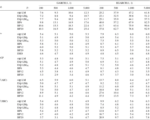
The results for the GARCH models are presented in Table2. The results show that the differences between the true and nom-inal levels are substantial when the identity matrix is used. The differences are largest for the BP tests with the EGARCH(1,1)
model. The differences tend to increase as the sample size in-creases. The increase is large for the EGARCH(1,1).
Next we consider the generalized tests in Table2. We first compare the LM-based tests. The differences between the true and nominal levels tend to be essentially eliminated for GARCH(1,1) when the tests use the consistent estimators
ˆ
V∗,VˆGPorVˆ(SBC)andT≥500. For EGARCH(1,1), the dif-ference is essentially eliminated when the tests use the con-sistent estimatorsVˆGPor Vˆ(SBC)andT ≥500. In both cases larger sample sizes are needed to eliminate the difference when
ˆ
V(AIC) is used, especially for the sup LM test. Overall, the Exp-LM0and Exp-LM∞tests tend to have better control over
the level than the sup LM tests. The estimator ofVˆ∗is inconsis-tent in the EGARCH case. The results forVˆ∗in Table2show only a small tendency for over rejection atT=1,000 because
the average off-diagonal elements ofVare close to zero at this sample size.
Next consider other tests. The generalized BP tests generally tend to show less satisfactory control over the level than the LM-based tests, especially BP20. The levels of the Deo (2000) test are similar to those of the generalized LM tests in theV∗ case. We also calculated the finite-sample rejection probabil-ities using the skewed t(5)GARCH(1,1)using the standard-ized version given in Lambert and Laurent (2001) and the mix-tures of normal GARCH(1,1)proposed by Haas, Mittnik, and Paolella (2004). The previous conclusions are not altered by the results for these latter models.
The location model (18) is also used for the power compar-isons, but now with serially correlated errors. Following AP, the models used for the errorsεtinclude
AR(1): εt=φεt−1+ut,
MA(1): εt=ut+θut−1,
AR(6): εt=φ
6
j=1
7−j
6 εt−j+ut,
(19)
AR(12): εt=φ
12
j=1
13−j
12 εt−j+ut,
AR(6)± : εt=φ
6
j=1
(−1)j+17−j
6 εt−j+ut,
AR(12)± : εt=φ
12
j=1
(−1)j+113−j
12 εt−j+ut.
The above models were chosen by AP because they include a wide variety of patterns of serial correlation with both positive and negative serial correlations. The models used for the inno-vations ut are the GARCH(1,1) and EGARCH(1,1) models
and the nonlinear moving average and bilinear models. We calculated the 0.05 level-corrected powers by simulation for sample sizeT=1,000 using 25,000 replications. The finite-sample critical values are simulated using 25,000 replications. The parameter values are chosen so that the maximum pow-ers are approximately 0.4 and 0.8 for the two parameter values considered. All models are simulated with an approximately stationary startup by taking the last T random variables from a simulated sequence of theT+500 random variables where startup values are set equal to zero.
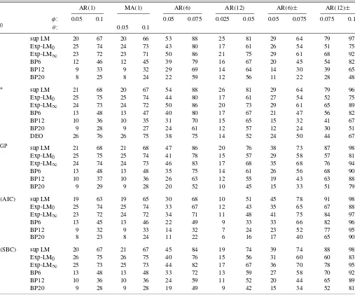
Table 3 presents the 0.05 level-corrected power of each of the tests for the AR(1), MA(1), AR(6), AR(12), AR(6)±, and AR(12)±models with GARCH(1,1)innovations.
The powers in Table3present a mixed picture. A compari-son of the LM-based tests shows that Exp-LM0tends to have
the highest power for the AR(1)and MA(1)models and the lowest power for the AR(12), AR(6)±, and AR(12)±models. For the latter models, the sup LM test has the highest power. We conclude that the sup LM test has higher all-around power than the Exp-LM∞by a small margin. The same pattern tends to hold when different values ofφandθ are used in the error models.
252 Journal of Business & Economic Statistics, April 2010
Table 2. Rejection probabilities (percent) of nominal 0.05 tests: MDS models
GARCH(1,1) EGARCH(1,1)
ˆ
V0 T: 200 500 1,000 5,000 200 500 1,000 5,000
I sup LM 7.6 9.3 10.6 12.3 25.2 37.9 47.2 61.8
Exp-LM0 7.2 8.8 9.4 10.7 23.1 32.5 39.8 51.2
Exp-LM∞ 7.7 9.4 10.2 11.7 25.1 35.9 44.1 57.3
BP6 9.8 13.1 14.9 17.6 40.0 57.2 67.9 82.5
BP12 10.6 15.3 18.3 22.4 41.7 63.4 75.9 90.6
BP20 10.3 16.5 20.6 25.4 37.8 62.7 76.8 92.9
ˆ
V∗ sup LM 5.4 5.1 5.0 5.3 7.9 6.3 6.0 6.0
Exp-LM0 5.1 4.9 4.9 5.0 6.9 5.4 5.1 5.3
Exp-LM∞ 5.3 5.0 5.0 5.2 7.5 5.9 5.5 5.6
BP6 5.8 5.1 4.8 4.9 8.7 6.1 5.3 4.9
BP12 6.0 5.2 5.0 5.1 9.3 6.7 5.7 5.0
BP20 5.8 5.2 5.2 5.2 8.9 6.5 5.9 5.4
DEO 4.6 4.7 4.8 4.9 4.8 4.5 4.6 4.8
ˆ
VGP sup LM 5.3 4.8 5.0 5.1 7.5 5.1 4.8 4.2
Exp-LM0 5.1 4.7 4.9 5.0 6.9 5.1 4.7 4.8
Exp-LM∞ 5.2 4.8 4.9 5.1 7.2 5.0 4.6 4.5
BP6 5.3 4.4 4.6 4.7 8.1 4.8 4.1 3.9
BP12 4.5 3.8 4.1 4.9 8.7 4.3 3.4 3.5
BP20 3.3 2.9 3.4 4.6 8.7 3.7 3.0 3.6
ˆ
V(AIC) sup LM 6.5 5.9 6.0 5.1 13.7 8.0 6.4 6.7
Exp-LM0 5.0 4.7 4.7 4.7 9.2 5.2 4.2 4.7
Exp-LM∞ 5.6 5.1 5.1 4.9 11.2 6.0 4.9 5.4
BP6 7.0 5.0 4.7 4.5 18.8 8.0 5.1 5.3
BP12 8.9 5.1 4.6 4.6 27.6 10.4 6.0 6.4
BP20 11.1 4.9 4.2 4.4 37.5 13.5 7.3 8.7
ˆ
V(SBC) sup LM 5.4 4.9 5.1 4.9 9.9 6.2 5.6 6.3
Exp-LM0 5.0 4.6 4.8 5.0 7.4 4.8 4.1 4.4
Exp-LM∞ 5.2 4.8 4.8 5.0 8.5 5.2 4.5 5.0
BP6 5.4 4.5 4.7 4.7 12.8 6.7 4.8 4.8
BP12 4.7 4.0 4.2 4.9 16.7 8.1 5.4 5.9
BP20 3.7 3.1 3.6 4.7 20.9 9.7 6.5 7.8
NOTE: The tests, as functions ofVˆ0, are defined in (12) and (14) above. The estimatorVˆ∗is consistent in the diagonal MDS case;VˆGPis consistent for general MDS processes;
the estimatorsVˆ(AIC)andVˆ(SBC)are consistent estimators in both MDS and non-MDS cases. DEO refers to the Deo (2000) test, which is consistent in the diagonal MDS case. The number of replications is 25,000.
Among the BP tests, the BP6 has the highest power. The sup LM test has higher power than the BP6 test and by a consid-erable margin in many cases. The powers of the BP6 test tend to be higher than the powers of the Exp-LM0for the AR(12)±
model. The powers of the BP6 test are lower than the powers of the Exp-LM∞test. The power of the Deo (2000) test is slightly higher than the power of the generalized AP tests in the AR(1)
and MA(1)cases, but in other cases it is smaller and sometimes substantially so.
When the powers of the tests are compared for models with EGARCH(1,1)innovations, our conclusions are essentially the same as those for GARCH(1,1), and similarly for the models with nonlinear moving average innovations and with bilinear innovations.
Following AP, we also investigated the 0.05 level-corrected powers where ARMA(1,1)models are used for the errors. As previously, the innovationsutare generated by the MDS or
non-MDS models considered previously. In simulation experiments where ARMA(1,1)models are used for the errors, the sup LM tests no longer have the best all-around power compared to the
Exp-LM0 and Exp-LM∞tests. Once the results from ARMA
error models are taken into account, the sup LM, Exp-LM0,
and Exp-LM∞tests all have better power than the BP tests, but none is dominant.
Of course, the power results are influenced by the models and parameter values used in the simulation experiments. Note that the data generation processes used in the above experi-ments have declining weights as the lag length increases. As a consequence, the first autocorrelation is dominant. This type of design is relevant for applications in economics and finance. As we have seen, for this type the generalized AP tests tend to have higher power than the generalized BP tests. However, the reverse can be hold for designs where the first autocorrelation is not important. A simple example of a data generation process with this property is an AR(2)where the coefficient onYt−1is
zero and onYt−2is negative. This caveat should be kept in mind
when interpreting the results.
AP considered seasonal MA models for the errors εt. The
models are
MA(j): εt=ut+θut−j, j=1, . . . ,6. (20)
Table 3. Level-corrected powers of 0.05 tests for AR and MA models with GARCH(1,1)errors,T=1,000
AR(1) MA(1) AR(6) AR(12) AR(6)± AR(12)±
φ: 0.05 0.1 0.05 0.075 0.025 0.05 0.05 0.075 0.075 0.1
ˆ
V0 θ: 0.05 0.1
I sup LM 20 67 20 66 53 88 25 81 29 64 79 97
Exp-LM0 25 74 24 73 43 80 17 61 26 54 51 75
Exp-LM∞ 23 72 23 71 50 86 21 75 29 61 68 92
BP6 12 46 12 45 39 79 16 67 20 45 54 82
BP12 9 33 9 32 29 69 14 64 14 30 39 65
BP20 8 25 8 24 22 59 12 56 11 22 28 48
ˆ
V∗ sup LM 21 68 20 67 54 88 26 81 29 64 79 96
Exp-LM0 25 75 25 74 44 80 17 61 27 54 52 75
Exp-LM∞ 24 73 24 72 50 86 20 73 29 61 65 89
BP6 13 48 13 47 40 80 17 67 21 47 56 82
BP12 10 36 10 35 31 70 15 65 15 32 41 67
BP20 9 28 9 27 24 61 12 57 12 24 30 51
DEO 26 76 26 75 38 75 14 52 24 50 44 67
ˆ
VGP sup LM 21 68 21 68 47 86 20 76 38 73 87 98
Exp-LM0 25 75 25 74 41 78 15 57 29 58 57 81
Exp-LM∞ 24 74 24 73 46 83 17 68 35 68 76 94
BP6 13 48 13 48 35 75 14 61 26 56 68 90
BP12 10 37 10 36 26 63 12 55 19 43 63 88
BP20 9 29 9 28 20 52 10 45 15 33 51 79
ˆ
V(AIC) sup LM 19 63 19 65 30 68 10 51 45 78 91 98
Exp-LM0 25 74 25 74 33 67 12 43 35 65 67 88
Exp-LM∞ 23 72 24 72 34 71 11 48 41 75 84 97
BP6 13 45 13 46 22 49 9 33 33 66 82 96
BP12 9 32 9 33 14 32 7 24 23 52 77 95
BP20 8 23 8 24 11 22 6 16 17 40 65 90
ˆ
V(SBC) sup LM 20 67 21 67 45 84 19 74 39 74 88 98
Exp-LM0 26 75 26 75 40 76 15 56 31 60 60 83
Exp-LM∞ 25 73 25 73 44 82 17 67 36 70 78 95
BP6 13 48 13 48 33 72 13 59 27 58 70 92
BP12 10 36 10 36 24 59 11 52 20 44 65 89
BP20 9 28 9 28 19 49 9 42 15 34 52 81
NOTE: See Table2. The number of replications is 25,000.
We calculated the 0.05 level corrected power for these er-ror models withθ =0.15 where the ut are generated by the
EGARCH(1,1)model. For the seasonal models, the BP6 and B12 tests are best of those considered, with BP6 test having the highest all around power. This conclusion is the same as that reached by AP.
AP implement the tests using Tr=50 and we do so using
Tr=20. We investigated whether this affects the consistency
of the tests. We found that with|| ≤0.8 and a process with
ρ1= · · · =ρ20=0, ρ21=0 increasing the truncation lag does not make any very noticeable difference to powers and thus the consistency of the tests as the sample sizeTincreases to 15,000. Further, we simulated the level-corrected powers forT=1,000 usingTr=40. The powers of the LM-based tests forTr=40
are essentially the same forTr=20, and hence the conclusions
from the power comparisons are unchanged.
Computing. The random number generator used in the ex-periments was the very long period generator RANLUX with luxury levelp=3; see Hamilton and James (1997). The pro-gram used for VARHAC was the version of the propro-gram by
den Haan and Levin (http:// econ.ucsd.edu/ ~wdenhaan/ varhac. html) modified to run substantially faster.
6. EMPIRICAL APPLICATION
As Campbell, Lo, and MacKinlay (1997) note, the pre-dictability of stock returns is an active research topic. They il-lustrate the empirical relevance of predictability by applying the BP tests to CRSP stock return indexes. In this section, their em-pirical application is extended in two ways: First, results are presented for the AP tests as well as the generalized AP and BP tests; second, results are presented for an extension of their sample period.
Campbell, Lo, and MacKinlay (1997) report the means, stan-dard deviations, the first four sample autocorrelations (in per-cent) as well as the BP5 and BP10 statistics in their table 2.4
for monthly, weekly, and daily value-weighted (VWRETD) and equal-weighted (EWRETD) stock return indexes (NYSE/ AMEX). The sample period is July 3, 1962 to December 31,
254 Journal of Business & Economic Statistics, April 2010
1994. We replicated the results by Campbell, Lo, and MacKin-lay (1997) for this sample period and the subperiods they se-lected.
In this section, the sample period is July 3, 1962 to Decem-ber 30, 2005. Results were calculated for the sup LM, Exp-LM0, and Exp-LM∞tests, and the generalized AP and BP tests,
both for the sample period and subperiods considered by Camp-bell, Lo, and MacKinlay (1997) and for the extended sample period and selected subperiods. The skewness and kurtosis sta-tistics were also calculated to provide a check on the normality of the returns. As expected, the kurtosis statistics provide strong evidence against normality.
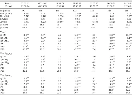
For the sake of brevity, we only report results for the monthly equal-weighted stock return indexes. Table4illustrates that in-ferences from the generalized AP tests can conflict with those from the generalized BP tests. The generalized AP tests tend to reject and the generalized BP tests tend not to reject. For the data used by Campbell, Lo, and MacKinlay (1997), the BP tests tend to not reject at the nominal 0.05 level and similarly for the generalized BP tests. The greater number of rejections by the generalized AP tests may be explained by the higher power of the generalized AP tests compared to the generalized BP tests.
Table 4 also shows that both the AP and BP tests tend to reject at the nominal 0.05 and or 0.01 levels for the extended
sample period and selected subperiods. The same is true for the generalized AP tests. Again, there are substantially fewer rejections by the generalized BP tests than the generalized AP tests.
In light of our Monte Carlo experiments, the results reported by Campbell, Lo, and MacKinlay (1997) for the BP tests are difficult to interpret in isolation. Although the BP statistics are often enormous for weekly and daily data, this alone does not provide strong evidence that the null of zero correlation is false. This is because the BP tests tend to substantially over-reject when data are generated by uncorrelated dependent processes such as a GARCH(1,1)or EGARCH(1,1)model. In particular, the over-rejection is most pronounced for large sample sizes, sizes similar to those in this empirical application.
The motivation of the empirical application is predictability of stock returns, which is characterized by a MDS condition in stock returns. The MDS hypothesis implies that stock returns are white noises, so it is valid to use tests for serial correlation in testing the predictability of stock returns. Hence, robustness under conditional heteroscedasticity in the case of GARCH and EGARCH is an appealing property of the generalized AP test. However, robustness under the non-MDS cases (nonlinear MA and bilinear) may be interpreted as a drawback for this purpose because non-MDS processes which can be used for prediction will be missed.
Table 4. Tests of serial correlation in monthly CRSP EWRETD stock index returns
Sample: 07:31:62 07:31:62 10:31:78 07:03:62 01:03:95 10:30:78 01:29:88
Period: 12:30:94 09:29:78 12:30:94 12:30:05 12:30:05 12:30:05 12:30:05
Sample size 390 195 195 522 132 326 216
Mean (×100) 1.077 1.05 1.104 1.089 1.122 1.18 1.06
SD (×100) 5.749 6.148 5.336 5.357 4.001 4.68 3.957
Skewness −0.45 0.30 −1.59 −0.54 −1.11 −1.40 −0.72
Kurtosis 7.367 5.299 10.607 7.821 6.734 10.625 5.753
ˆ
ρ1(×100) 17.1 18.4 15 17.5 19.7 18.8 23.2
ˆ
ρ2(×100) −3.4 −2.5 −1.6 −4.1 −8.4 −4.0 −3.0
ˆ
V0=I
sup LM 11.8∗∗ 6.8∗ 4.4 16.6∗∗ 5.8 11.8∗∗ 11.8∗∗
Exp-LM0 8.6∗∗ 5.7∗∗ 2.7 11.9∗∗ 3.8∗ 8.0∗∗ 8.1∗∗
Exp-LM∞ 5.0∗∗ 2.9∗ 1.6 7.2∗∗ 2.3∗ 4.9∗∗ 5.0∗∗
BP5 12.8∗ 7.4 8.7 18.6∗∗ 10.3 19.9∗∗ 19.9∗∗
BP10 20.9∗ 12.3 13.7 27.8∗∗ 12.1 26.5∗∗ 21.3∗
BP20 40.7∗∗ 30.6 20.4 47.7∗∗ 17.6 32.7∗ 27.5
ˆ
V0= ˆV(AIC)
sup LM 9.5∗∗ 6.4∗ 2.7 13.8∗∗ 3.0 1.9∗∗ 8.3∗
Exp-LM0 7.4∗∗ 4.7∗ 2.0 10.3∗∗ 1.4 6.9∗∗ 5.2∗
Exp-LM∞ 4.1∗∗ 2.6∗ 1.0 6.1∗∗ 0.9 4.1∗∗ 3.3∗
BP5 9.8 6.5 3.8 14.2∗ 5.4 13.1∗ 10.6
BP10 16.5 8 8.6 20.0∗ 7.3 19.1∗ 11.1
BP20 22.2 13.4 25.5 26.0 11.1 24.5 15.9
ˆ
V0= ˆV(SBC)
sup LM 9.4∗∗ 5.0 3.5 13.3∗∗ 5.3 11.3∗∗ 8.4∗
Exp-LM0 6.3∗∗ 3.6∗ 2.3 9.0∗∗ 3.3 6.9∗∗ 5.5∗
Exp-LM∞ 3.8∗∗ 2.0 1.3 5.6∗∗ 2.0∗ 4.3∗∗ 3.4∗∗
BP5 11.0 5.1 7.4 16.1∗∗ 7.5 15.3∗∗ 11.8∗
BP10 17.0 9.7 12.6 22.6∗ 10.8 22.2∗ 12.2
BP20 24.4 16.9 22.7 29.4 15.4 29.3 14.6
NOTE: See Table2for definitions of functions ofVˆ0. In the VARHAC procedure to compute the generalized statistics the maximum lag is set at int(T0.25). One and two stars denote
rejection at the nominal 0.05 and 0.01 levels, respectively.
7. CONCLUDING COMMENTS
In the simulations in this paper, the differences between the true and nominal levels of the generalized AP tests are es-sentially zero for suitable sample sizes, and the generalized AP tests have good power properties for nonseasonal alter-natives compared to the generalized Box–Pierce tests and the Deo (2000) tests. The Exp-LM∞test is recommended for non-seasonal applications in economics and finance. The paper in-cludes an empirical application to stock return indexes that is motivated by the search for predictability in returns. The results illustrate that inferences from the generalized AP tests can con-flict with those from the generalized Box–Pierce tests and can make a difference to the inferences drawn from the data.
Andrews, Liu, and Ploberger (1998) extended their ap-proach to testing white noise against multiplicative seasonal ARMA(1,1)models. A topic for further research would be to use our approach to generalize the LM-based test for this case. The generalized LM-based tests do not apply to residuals from ARMA models. We plan to investigate this topic in future re-search.
ACKNOWLEDGMENTS
The authors gratefully acknowledge the helpful comments of the editor and referees. Don Andrews, John Geweke, and Ignacio Lobato provided useful advice.
[Received April 2008. Revised August 2008.]
REFERENCES
Akaike, H. (1973), “Information Theory and the Extension of Maximum Like-lihood Principle,” inSecond International Symposium on Information The-ory, eds. B. Petrov and F. Casaki, Budapest: Akailseoniai-Kiudo, pp. 267– 281. [250]
Andrews, B., Davis, R. A., and Breidt, F. J. (2006), “Maximum Likelihood Esti-mation for All-Pass Time Series Models,”Journal of Multivariate Analysis, 97, 1638–1659. [246]
Andrews, D. W. K., and Monahan, J. C. (1992), “An Improved Heteroskedas-ticity and Autocorrelation Consistent Covariance Matrix Estimator,” Econo-metrica, 60, 953–966. [250]
Andrews, D. W. K., and Ploberger, W. (1994), “Optimal Tests When a Nuisance Parameter Is Present Only Under the Alternative,”Econometrica, 62, 1383– 1414. [246,247]
(1995), “Admissibility of the Likelihood Ratio Test When a Nuisance Parameter Is Present Only Under the Alternative,”Annals of Statistics, 23, 1609–1609. [246]
(1996), “Testing for Serial Correlation Against an ARMA(1,1)
Process,”Journal of the American Statistical Association, 91, 1331–1342. [246]
Andrews, D. W. K., Liu, X., and Ploberger, W. (1998), “Tests for White Noise Against Alternatives With Both Seasonal and Nonseasonal Serial Correla-tion,”Biometrika, 85, 727–740. [255]
Bera, A. K., and Higgins, M. L. (1997), “ARCH and Bilinearity as Compet-ing Models for Nonlinear Dependence,”Journal of Business & Economic Statistics, 15, 43–51. [250,251]
Bollerslev, T. (1986), “Generalized Autoregressive Conditional Heteroskedas-ticity,”Journal of Econometrics, 31, 307–327. [250]
Box, G. E. P., and Pierce, D. A. (1970), “Distribution of Residual Autocorre-lations in Autoregressive Integrated Moving Average Time Series Models,”
Journal of the American Statistical Association, 93, 1509–1526. [246] Campbell, J. Y., Lo, A. W., and MacKinlay, A. C. (1997),The Econometrics
of Financial Markets, Princeton, NJ: Princeton University Press. [250,253,
254]
Chen, W. W., and Deo, R. S. (2004), “A General Portmanteau Goodness-of-Fit Test for Time Series Models,”Econometric Theory, 20, 382–416. [246]
Davidson, J. (2000), “When Is a Time SeriesI(0)? Evaluating the Memory Properties of Nonlinear Dynamic Models,” preprint, Cardiff University. [248]
De Jong, R. M., and Davidson, J. (2000), “The Functional Central Limit Theo-rem and Weak Convergence to Stochastic Integrals, Part 1: Weakly Depen-dent Processes,”Econometric Theory, 16, 621–642. [248]
Den Haan, W. J., and Levin, A. (1997), “A Practitioner’s Guide to Robust Co-variance Matrix Estimation,” inHandbook of Statistics: Robust Inference, eds. G. S. Maddala and C. R. Rao, Amsterdam: North-Holland, pp. 191– 341. [249]
(1998), “Vector Autoregressive Covariance Matrix Estimation,” manu-script, Dept. of Economics, University of California, San Diego. [249,250] Deo, R. S. (2000), “Spectral Tests of the Martingale Hypothesis Under Con-ditional Heteroskedasticity,”Journal of Econometrics, 99, 291–315. [246,
247,250-252,255]
Diebold, F. X. (1987), “Testing for Serial Correlation in the Presence of ARCH,”Proceedings of the Business and Economics Statistics Section, 1986, Washington: American Statistical Association, pp. 323–328. [250] Durlauf, S. (1991), “Spectral Based Testing for the Martingale Hypothesis,”
Journal of Econometrics, 50, 1–19. [246]
El Babsiri, M., and Zakoian, J.-M. (2001), “Contemporaneous Asymmetry in GARCH Processes,”Journal of Econometrics, 101, 257–294. [251] Francq, C., Roy, R., and Zakoian, J.-M. (2005), “Diagnostic Checking in
ARMA Models With Uncorrelated Errors,”Journal of the American Sta-tistical Association, 100, 532–544. [246,250]
Granger, C. W. J., and Andersen, A. P. (1978),An Introduction to Bilinear Time Series Models, Gottingen: Vanenhoek and Ruprecht. [251]
Guo, B. B., and Phillips, P. C. B. (1998), “Testing for Autocorrelation and Unit Roots in the Presence of Conditional Heteroskedasticity of Unknown Form,” manuscript, Cowles Foundation for Research in Economics, Yale University, New Haven. [250]
Haas, M., Mittnik, S., and Paolella, M. (2004), “Mixed Normal Conditional Heteroskedasticity,”Journal of Financial Econometrics, 2, 211–250. [251] Hamilton, K. G., and James, F. (1997), “Acceleration of RANLUX,”Computer
Physics Communications, 101, 241–248. [253]
He, C., and Teräsvirta, T. (1999), “Properties of Moments of a Family of GARCH Processes,”Journal of Econometrics, 92, 173–192. [250] He, C., Teräsvirta, T., and Malmsten, H. (2002), “Moment Structure of a
Fam-ily of First-Order Exponential GARCH Models,”Econometric Theory, 18, 868–885. [250]
Hong, Y. (1996), “Consistent Testing for Serial Correlation of Unknown Form,”
Econometrica, 64, 837–864. [246]
Hong, Y., and Lee, Y. J. (2003), “Consistent Testing for Serial Correlation of Unknown Form Under General Conditional Heteroskedasticity,” technical report, Depts. of Economics and Statistical Sciences, Cornell University. [246]
Lambert, P., and Laurent, S. (2001), “Modelling Financial Time Series Using GARCH-Type Models With a Skewed Student Distribution for the Innova-tions,” working paper, Universite Catholique de Louvain and Universite de Liege. [251]
Lo, A. W., and MacKinlay, A. C. (1989), “The Size and Power of the Vari-ance Ratio Test in Finite Samples: A Monte Carlo Investigation,”Journal of Econometrics, 40, 203–238. [250]
Lobato, I., Nankervis, J. C., and Savin, N. E. (2001), “Testing for Autocorrela-tion Using a Modified Box–PierceQTest,”International Economic Review, 42, 187–205. [250]
(2002), “Testing for Zero Autocorrelation in the Presence of Statistical Dependence,”Econometric Theory, 18, 730–743. [246-249]
Poterba, J. M., and Summers, L. H. (1988), “Mean Reversion in Stock Prices: Evidence and Implications,”Journal of Financial Economics, 22, 27–59. [246]
Pötscher, B. M. (1990), “Estimation of Autoregressive Moving-Average Order Given an Infinite Number of Models and Approximation of Spectral Densi-ties,”Journal of Time Series Analysis, 11, 165–179. [246]
Romano, J. L., and Thombs, L. A. (1996), “Inference for Autocorrelations Un-der Weak Assumptions,”Journal of the American Statistical Association, 91, 590–600. [248]
Schwartz, G. (1978), “Estimating the Dimension of a Model,”Annals of Statis-tics, 6, 461–464. [250]
Taylor, S. (1984), “Estimating the Variances of Autocorrelations Calculated From Financial Time Series,”Applied Statistics, 33, 300–308. [250] Taylor, S. J. (2005),Asset Price Dynamics, Volatility, and Prediction, Princeton,
NJ: Princeton University Press. [246]
Tong, H. (1990), Nonlinear Time Series, Oxford: Oxford University Press. [251]