Deborah A. Cobb-Clark
Vincent A. Hildebrand
a b s t r a c t
This paper analyzes the sources of disparities in the relative wealth position of Mexican Americans. Results reveal that—unlike the racial wealth gap— Mexican Americans’ wealth disadvantage is in large part not the result of differences in wealth distributions conditional on the underlying determi-nants of wealth. Rather, Mexican Americans’ wealth disadvantage is attrib-utable to the fact that these families have more young children and heads who are younger. Mexican Americans’ low educational attainment also has a direct effect in producing a wealth gap relative to other ethnic groups even after differences in income are taken into account. Income differentials are important, but do not play the primary role in explaining the gap in median net worth. Finally, geographic concentration is generally unimportant, but does contribute to narrowing the wealth gap between wealthy Mexican Americans and their white and black counterparts.
I. Introduction
Over the decade of the 1990s, more than 2.2 million immigrants to the United States—approximately one in four—came from Mexico. Many other Mexicans entered the United States as temporary residents, while the Mexican popu-lation illegally resident in the United States has been estimated to be increasing by just over 150,000 individuals each year (USINS 2002: Tables 2 and 4). This large-scale migration of Mexicans in conjunction with relatively high fertility rates has made Mexican Americans one of the fastest growing ethnic groups in the United
Deborah Cobb-Clark is a professor of economics in the Research School of Social Sciences at the Australian National University and a research fellow at the Institute for the Study of Labor (IZA). Vincent Hildebrand is an assistant professor of economics at Glendon College (York University) and a research fellow at CEPS/INSTEAD. The authors would like to thank David Jaeger and two anonymous referees for many useful comments. Vincent Hildebrand acknowledges support from the Social and Economic Dimensions of an Aging Population (SEDAP) Research Program. The data used in this article can be obtained beginning February 2007 through January 2010 from Vincent Hildebrand, Department of Economics, Glendon College, 2275 Bayview Ave., Toronto, Ontario, M4N3M6, Canada. E-mail: vincent@econ.yorku.ca
[Submitted August 2005; accepted March 2006]
States. Between the 1990 and 2000 censuses, the Mexican American population grew by 52.9 percent, while the overall U.S. population increased by 13.2 percent and the white, non-Hispanic population grew by just 3.4 percent (U.S. Census Bureau 2001b). This paper contributes to the emerging literature on the economic well-being of Mexican Americans by analyzing the factors related to their relative wealth position. With an average household income that is more than 40 percent below that of non-Hispanic whites, Mexican Americans are one of the most economically disadvantaged groups in the United States (Grogger and Trejo 2002). The low income of Mexican American families appears to stem primarily from low wages—as opposed to lower participation rates, higher unemployment rates, or shorter work weeks (Reimers 1984; Trejo 1997)—and many authors point to a relative lack of formal education as the pri-mary cause of the wage gap between Mexican Americans and other workers (Trejo 1997; Grogger and Trejo 2002). As a group, Hispanics also have lower levels of net worth (for example, Hao 2003; Wakita, Fitzsimmons, and Liao 2000; Wolff 2000; Choudhury 2001; Smith 1995), are more likely to live in poverty (U.S. Census Bureau 1995), and are less likely to hold their wealth in the form of housing, financial assets, or business capital (for example, Borjas 2002; Bertaut and Starr-McCluer 1999; Fairlie and Woodruff 2005; Osili and Paulson 2003; Smith 1995).
Though the source of the racial wealth gap has been a matter of debate (see Blau and Graham 1990; Gittleman and Wolff 2000; Menchik and Jianakoplos 1997; Chiteji and Stafford 1999), less is known about the factors driving the wealth position of Mexican Americans. While it seems reasonable to expect that low wealth levels and low earnings are related, this link has not been formally established in the literature. Indeed, there are many other factors that also might lead the wealth of Mexican Americans to be lower than that of other groups. Hispanics as a group are younger, less likely to be married, and have larger numbers of children than other groups (U.S. Bureau of the Census 1995; 2001a; 2001b). These demographic differences—which are directly related to stage of the life cycle—are likely to be important in determin-ing the net worth position of Mexican Americans. Furthermore, although becomdetermin-ing more geographically diffuse over time (Guzman and Diaz McConnell 2002), two thirds of Mexican Americans live in just two states—California and Texas (U.S. Bureau of the Census 2001b)—raising the possibility that it is geographic clustering and the characteristics of specific housing markets that lie behind a lower propensity to hold wealth in the form of housing.
market opportunities (Grogger and Trejo 2002). Disparity in earnings potential and differential incentives to save and consume out of current income imply that both the level of wealth and the portfolio choices of immigrants are likely to differ from those of the native-born (Amuedo-Dorantes and Pozo 2002; Cobb-Clark and Hildebrand 2006a, 2006b).
This paper analyzes the sources of disparities in the relative wealth position of Mexican Americans using the Survey of Income Program Participation (SIPP) data. These data are unique in providing information on both household wealth holdings and immigration history allowing us to separately consider the wealth of foreign- and U.S.-born Mexican Americans. This level of disaggregation is a significant advantage over previous research that tends to consider Hispanics as a single group. We pursue a semi-parametric decomposition approach proposed by DiNardo, Fortin, and Lemieux (1996) that—unlike the standard Oaxaca (1973) and Blinder (1973) approach—allows us to consider the entire wealth distribution. This enables us to decompose the wealth gap into its various components at multiple points (in our case, the 10th, 25th, 50th, 75th, and 90th percentiles) of the distribution and to consider a decomposition of the relative spread (for example, the 50–10 gap) of wealth.
Our results reveal that—unlike the racial wealth gap—Mexican Americans’ wealth disadvantage is in large part not the result of differences in wealth distributions condi-tional the underlying determinants of wealth. Rather, Mexican Americans’ wealth dis-advantage is attributable to the fact that these families have more young children and heads who are younger. Mexican Americans’ low educational attainment also has a direct effect in producing a wealth gap relative to other ethnic groups even after differences in income are taken into account. Income differentials are important, but do not play the primary role in explaining the gap in median net worth. Finally, geographic concentration is generally unimportant, but does contribute to narrowing the wealth gap between wealthy Mexican Americans and their white and black counterparts.
II. The Survey of Income and Program Participation
This paper exploits data drawn from the 1984, 1985, 1987, 1990–1993, 1996, and 2001 surveys of the Survey of Income and Program Participation (SIPP). Each survey is a short, rotating panel made up of eight to 12 waves of data—collected every four months—for approximately 14,000 to 36,700 U.S. households. Thus, a typical survey year covers a time span ranging from 2 1/2 to four years. Most SIPP panels did not sample different subpopulations at different rates, however, the 1990 and 1996 panels are exceptions and consequently we used the relevant sample weights in our estimation. Each wave of the survey contains both core questions that are common to each wave and topical questions about a particular topic that are not updated in each wave. In our case, immigration information is usu-ally collected in the second wave of each survey, while household wealth information is generally collected in Wave 4 or Wave 7.
upper tail of the wealth distribution particularly poorly (see Juster and Kuester 1991; Wolff 1998; Juster, Smith, and Stafford 1999). Unfortunately, SCF data do not iden-tify foreign-born individuals. The Panel Survey of Income Dynamics (PSID) is an alternative data source that does collect information about immigration histories. Given its sampling frame, however, the PSID is not particularly useful for studying the foreign-born population in the United States before 1998 when a representative sample of 491 immigrant families was added to the survey. The Health and Retirement Survey (HRS) provides wealth information and identifies immigrants. However, HRS data lack region of origin information and are restricted to households whose head was between 51 and 62 years in 1992 the initial year of data collection. Similarly, National Longitudinal Survey (NLS) and National Longitudinal Survey of Youth (NLSY) data shed light only on the wealth holdings of specific birth cohorts.
Given the heterogeneity within the Mexican American population it is important to control for nativity. By pooling data from all of the years in which the SIPP collected both wealth and immigration information, we are able to build a data set that contains a much larger number of native-born and foreign-born Mexican American households than the PSID or NLSY. While our data will have little to say about the wealth hold-ings of the very rich, they are quite useful for studying the behavior of the middle class (Wolff 1998).
The SIPP wealth data come from a topical module on household assets and liabili-ties. Specific asset variables contained in the SIPP data include: interest earning assets held in banking and other institutions, equity in stocks and mutual fund shares, IRA and KEOGH accounts, own home equity, other real estate equity, business equity, net equity in vehicles, and other assets not accounted for including total mortgages held, money owed for the sale of businesses, U.S. savings bonds, checking accounts, and other interest-bearing assets. Liabilities include both debts secured by any assets and unsecured debts such as credit card or store bills, bank loans, and other unsecured debts. The SIPP wealth module, however, does not cover any future pension rights such as equity in private pension plans or social security wealth. Like other wealth surveys, the SIPP wealth module also does not specifically gather information about assets held off-shore which may be particularly relevant for foreign-born households.
Our estimation sample includes couple-headed, native-born, and foreign-born households in which the reference person is between 25 years and 75 years old. Native-born households in our sample are white, black, or Mexican American. A household is considered to be white if both partners self-identify as being white of non-Hispanic origin.1Black households include all households in which both partners
are native-born and self-identify as blacks. Native-born Mexican American house-holds include all househouse-holds whose respondents are native-born and identify them-selves either as being of Mexican-American, Chicano, or Mexican origin or descent. Foreign-born Mexican American households are those households in which both
partners are born in Mexico to non-U.S. parents. We have eliminated from our sample 1,075 mixed, native-born households and 676 mixed, foreign-born Mexican American households.2The resulting sample contains a total of 65,267 native-born,
couple-headed households and 1,499 Mexican-born, couple-headed households. Amongst the 65,267 native-born households 59,328 are white, 4,778 are black, and 1,161 are Mexican American.
We have restricted our analysis to couples because the SIPP like other surveys mea-sures household rather than individual wealth. Given the inherent differences in the ways in which partnered and single individuals make savings, consumption, and investment decisions, we believe it is more appropriate to analyze the wealth levels holdings of couples and singles separately. At the same time, there are ethnic and racial differences in the propensity to be partnered. Approximately two-thirds of the white (62 percent) and foreign-born Mexican American households (65 percent) in the SIPP are couples, while the proportions of blacks (33 percent) and native-born Mexican Americans (47 percent) who live in couples is much smaller. Although a full analysis of single-headed households is a topic for future research, preliminary estimation using data for single individuals suggests that our main conclusions are not driven by the differential propensity of different racial and ethnic groups to be partnered.
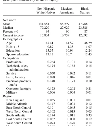
Table 1 reports for each ethnic group, weighted mean and median household net worth, mean household current income, and mean household demographic character-istics. As expected, both the mean and the median net worth of native-born house-holds reveal a great deal of heterogeneity across ethnic groups. In particular, the mean net worth of white households ($141,581) is more than twice that of both Mexican Americans ($58,299) and black ($47,768) households. Black households are the least well-off among all native-born households with a median net wealth ($23,585) about three times lower than that of whites ($79,220). However, Table 1 also reveals that black households are nevertheless doing substantially better than foreign-born, Mexican American households whose mean ($29,642) and median net worth ($6,792) are substantially lower than that of blacks. As expected, white households have the highest average current income ($15,834) of all groups considered. Interestingly, the average current income of black households ($12,092) is higher than that of both native-born ($10,759) and foreign-born Mexican Americans ($6,988). Foreign-born Mexican Americans are by far the most disadvantaged group both in terms of wealth holdings and current income.
To illustrate how wealth varies across the distribution, we plot the empirical cumu-lative distribution of net worth for each group in Figure 1. These are the wealth gaps we are seeking to explain. The difference in the net worth position of white house-holds at one extreme and foreign-born Mexican American househouse-holds at the other is striking. The vast majority (almost 95 percent) of white households hold positive lev-els of net worth, while this is true of many fewer of those families that have migrated
Table 1
Descriptive Statistics by Ethnic Grouping
Non-Hispanic Mexican Black Foreign-Born White Natives Americans Natives Mexicans Net worth
Mean 141,581 58,299 47,768 29,642
Median 79,220 27,929 23,585 6,792
Percent > 0 94 90 87 83
Current income 15,834 10,759 12,092 6,988
Demographics
Age 47.41 44.57 46.29 40.33
Kids < 18 0.89 1.35 1.07 2.12
Education 13.35 10.94 12.24 8.01
Spouse education 13.13 10.7 12.45 7.89
Occupations
Professional 0.264 0.101 0.141 0.029
Technical, sales, 0.174 0.163 0.157 0.06
administration
Service 0.050 0.092 0.112 0.129
Farm, forestry 0.028 0.046 0.018 0.12
Precision products, 0.140 0.173 0.106 0.192
crafts
Operators-laborers 0.123 0.202 0.212 0.275
Military 0.006 0.004 0.018 0.001
Region
New England 0.055 0.001 0.014 0.001
Middle Atlantic 0.147 0.003 0.12 0.009
East North Central 0.19 0.045 0.154 0.081
West North Central 0.102 0.013 0.031 0.008
South Atlantic 0.174 0.011 0.33 0.025
East South Central 0.067 0.000 0.122 0.001
West South Central 0.094 0.476 0.148 0.23
Mountain 0.049 0.101 0.013 0.061
Pacific 0.114 0.345 0.064 0.583
Year of entry
<1965 0.114
1965–74 0.247
1975–84 0.359
>1985 0.281
N 59,328 1,161 4,778 1,499
to the United States from Mexico. Native-born Mexican American and black house-holds on the other hand have cumulative net worth distributions that appear much more similar. Native-born Mexican Americans have a wealth advantage over black households, though the difference is small—approximately $5,000 at the median (see Table 1).
Households’ demographic characteristics reveal that foreign- and native-born Mexican American households are on average younger, less educated, and have more children under the age of 18 than both white and black households. Foreign-born Mexican Americans have a particularly low level of educational achievement with an average of about eight years for the head compared to averages of 13.4, 11, and 12.2 for white, native-born Mexican American and black households respectively. In addi-tion, native-born and foreign-born Mexican Americans are more likely to hold blue-collar jobs than both white and black households. Finally, not surprisingly, both native-born and foreign-born Mexican Americans are mostly concentrated in the West South Central (including Texas) and the Pacific (including California) census regions while a large share of black households resides in the South Atlantic region.
III. Estimation Methodology
Our interest is in developing an estimation strategy that allows us to shed light on the source of the wealth gap between Mexican Americans and other
0 .1 .2 .3 .4 .5 .6 .7 .8 .9 1
Cumulative Percentage of the Population
-100000 0 100,000 200,000 300,000 400,000
Household Total Net Worth
Whites Native-Born Mexican Americans
Blacks Foreign-Born Mexican Americans
Figure 1
groups. One obvious approach would be to use a standard Oaxaca-Blinder decomposi-tion to assign the difference in the mean net worth of Mexican Americans and some comparison group into one or more components that are explained by the households’ observed characteristics and another unexplained component that arises from differ-ences in accumulated wealth conditional on those observed characteristics. This is the approach that has widely been used in previous studies of the black-white wealth gap in the United States (see, for example, Blau and Graham 1990; Gittleman and Wolff 2000). In our case, the Oaxaca-Blinder decomposition is less than ideal for two reasons. First, it would require that we specify a parametric model of the relationship between wealth and our independent variables—most notably income. Barsky et al. (2002), however, argue that the relationship between wealth and income is of unknown, non-linear functional form that is difficult to parameterize. Unfortunately, the Oaxaca-Blinder decomposition will not yield valid results unless we can adequately approximate the wealth distribution over the relevant income range. Second, the large proportion of individuals with nonpositive net worth and the overall skewness of the wealth distribution itself imply that decomposing the gap in mean net worth may be less informative than decomposing other aspects of the gap in wealth distributions (for example, in the medians or in the proportion of individuals with positive net worth).
To avoid these difficulties, we pursue a semi-parametric decomposition approach proposed by DiNardo, Fortin, and Lemieux (1996). This approach is similar in spirit to the Oaxaca-Blinder decomposition in that we will be constructing a series of coun-terfactual wealth distributions. The difference between the actual wealth distributions of various groups and these counterfactual wealth distributions form the basis of the decompositions underlying our empirical results.
A. Decomposition of the Wealth Gap
We begin by defining M to be a dummy variable indicating group membership— which for convenience we shall refer to as Mexican American status. Further, wis wealth and zis a vector of wealth determinants. Each observation in our data is then drawn from some joint density function, f, over (w, z, M). The marginal distribution of wealth for group jcan be expressed as follows:
(1) fj(w)≡f (w | M =j)= ∫f(w,z | M =j)dz
= ∫f(w | z, M =j)fz(z | M =j)dz
where jequals 1 for Mexican Americans and 0 otherwise. Equation 1 expresses the marginal wealth distribution for group jas the product of two conditional distributions (see Greene 1997; DiNardo, Fortin, and Lemieux 1996).
In order to consider the source of disparities in the net worth of different groups, we will partition the vector of household wealth determinants (z) into four compo-nents: (1) income (y); (2) educational attainment (e); (3) geographic concentration (r); and (4) household demographic composition (c). These factors align closely with our review of the potential explanations for Mexican Americans’ relatively low level of net worth. (See Section I.) Thus, z= (y, e, r, c). Given this partitioning and the same logic as behind Equation 1, we can write the wealth distribution of group jas follows:
(2) fj(w)≡f(w | M =j)
= ∫y∫e∫r∫cf(w|y, e, r, c, M =j). fy | e, r, c(y|e, r, c, M =j).
fe|r, c(e|r, c, M =j) . fr|c(r|c, M =j) . fc(c|M =j)dydedrdc
Equation 2 involves five conditional densities. The first (f) is the conditional wealth distribution given our wealth determinants (z) and group membership (M), while the second (fy⎪e, r, c) is the conditional income distribution given education, geographic concentration, household demographics and group membership. Similarly, fe⎪r, cand fr⎪care the conditional education and geographic concentration distributions respec-tively. Finally, fccaptures the distribution of demographic characteristics conditional on group membership. When the conditional expectation is linear in its relevant argu-ments, these conditional densities are closely related to regression functions (see Butcher and DiNardo 2002). We can, therefore, loosely think of fas reflecting a set of wealth determinants and fy⎪ercas reflecting a set of income determinants, etc.3
Expressing the wealth distributions as we have in Equation 2 leads quite naturally to a series of interesting counterfactual wealth distributions. In particular, we can define the wealth distribution (fA) that would prevail if Mexican Americans retained their own conditional income distribution (fy⎪e, r, c), but had the same conditional dis-tributions of wealth, education, geographic concentration, and demographic charac-teristics as the comparison group. Specifically,
(3) fA(w)= ∫
y∫e∫r∫cf (w|y, e, r, c, M =0) . fy|e, r, c(y|e, r, c, M =1). fe|r, c(e|r, c, M =0) . fr|c(r|c, M =0) dydedrdc
Equation 3 will be useful in isolating the effect of income disparities on the wealth gap. It in effect answers the following question: what would the Mexican American wealth distribution look like if Mexican Americans faced their own conditional income distribution, but otherwise had the same distribution of the remaining wealth determinants and (conditional on z) accumulated wealth in the same way as others? This can then be compared to another wealth distribution (fB) that would result if Mexican Americans retained both their own conditional income and education distri-butions, but had the same conditional geographic concentration, demographic charac-teristics, and wealth distributions as the comparison group. Similarly, fCand fDare the counterfactual wealth distributions that result when—in addition—we also allow Mexican Americans to retain their own geographic concentration and geographic con-centration along with demographic characteristics respectively.
Using these counterfactual distributions, we can decompose the wealth gap between our comparison group and Mexican Americans in the following way: (4) f0(w)−f1(w)=[f0(w) −fA (w)] +[fA (w) −fB (w)] +[fB (w) −fC (w)]
+ [fC (w) −fD (w)] +[fD (w) −f1(w)]
3. We could, for example, also express the wealth distribution in terms of the distribution of demographic characteristics conditional on income, education, and geographic concentration, in other words fc⎪y, r, e, etc.
In the Equation 4, the first right-hand-side term captures the effect of disparities in conditional income distributions on the wealth gap. Similarly, the second term reflects the effect of differences in educational background, while the third and fourth capture the effects of geographic concentration and demographic composition respectively. Finally, the fifth term arises from differences between the conditional (on z) wealth distributions of Mexican Americans and the comparison group.
In order to implement the decomposition given in Equation 4 it is necessary to have estimates of counterfactual distributions fAthrough fD. DiNardo, Fortin, and Lemieux (1996) provide a method for obtaining these and other counterfactual distributions by reweighting the wealth distribution of our comparison group. Specifically, our first counterfactual wealth distribution can be constructed as follows:
(5) fA(w) = ∫
y∫e∫r∫c ψ y|ercf(w |y, e, r, c, M =0) .fy|e, r, c (y|e, r, c, M=0). fe|r, c (e |r, c, M =0) .fr | c, (r |c, M =0) .fc (r |c, M =0) dydedrdc where
(6) ψ y|e, r, c=
fy|e, r, c (y |e, r, c, M =1) fy|e, r, c (y |e, r, c, M =0)
In effect, the wealth distribution of the comparison group is simply reweighted by the ratio of conditional income distributions of the two groups. Following DiNardo, Fortin, and Lemieux (1996), we can write the reweighting factor required to produce the counterfactual wealth distribution fAas
(7) ψ y|e, r, c=
P(M = 1|y, e, r, c)P(M = 0|e, r, c) P(M = 0|y, e, r, c) P(M = 1|e, r, c)
Counterfactual distributions fB, fC, and fDare constructed similarly.
B. Alternative Decompositions
As with the standard Oaxaca-Blinder decomposition, the decomposition given by Equation 4 is not unique. Ultimately, choices about which decompositions are more use-ful depend on our ability to sensibly interpret the resulting components and to use them to better understand the source of the wealth gap. In our case, there are two separate issues. The first is whether we generate our counterfactual distributions by reweighting the wealth distribution of the comparison group or that of Mexican Americans. The sec-ond is the sequence in which we choose to consider the specific components of the vec-tor of wealth determinants (z). We will discuss each of these issues in turn.
It is well-known that the results of the standard Oaxaca-Blinder decomposition are often quite sensitive to whether one evaluates the difference in coefficients—the “unexplained” component—using the characteristics of the first group, the second group, or some weighted combination (see, Cotton 1988).4The same issue arises here.
In Equation 4 the difference in conditional wealth distributions (the fifth right-hand
side term) is evaluated using the conditional income and demographic distributions of Mexican Americans.5We also could have chosen to estimate our counterfactual
dis-tributions by reweighting the Mexican American wealth distribution rather than by reweighting that of the comparison group. This would have resulted in a decomposi-tion in which the disparity in condidecomposi-tional wealth distribudecomposi-tions was evaluated using the conditional income and demographic distributions of the comparison group.
In our data, Mexican Americans have a slight income disadvantage relative to Blacks. In all other cases, the income distribution of Mexican Americans is consider-ably narrower than that of the comparison groups we will be considering. In this case, reweighting the Mexican American wealth distribution would involve extrapolating the Mexican American conditional wealth distribution beyond the income range actu-ally observed in the data (Barsky et. al. 2002). In other words, while Equation 4 involves observable quantities, the alternative decomposition would require consider-able extrapolation. Given this, we have chosen in all cases to follow the procedure outlined in Section IIIA and create our counterfactual distributions by reweighting the wealth distribution of the comparison group.6
The second issue arises because we have explicitly accounted for several different components of the wealth gap.7The difficulty is that the proportion of the wealth gap
accounted for by each of these factors will depend on the sequence (or order) in which we consider them (DiNardo, Fortin, and Lemieux 1996). In particular, the counterfac-tual distribution given by fA(see Equation 3) is formed by taking the comparison group’s wealth distribution as specified in Equation 2 as the starting point and first replacing the conditional income distribution with that for Mexican Americans. Counterfactual dis-tribution fBtakes fAand also replaces the conditional education distribution with that of Mexican Americans. This process continues through the remaining factors until the decomposition given in Equation 4 is achieved. Thus, the decomposition in Equation 4 reflects one possible sequence—for example, first income, second education, third geo-graphic concentration, and last demogeo-graphic characteristics—in which the wealth deter-minants for Mexican Americans are substituted for those of the comparison group. There are, of course, many others. Moreover, the number of possible sequences to be considered increases dramatically as we add components to the vector of wealth deter-minants. Using Equation 2 to decompose the wealth gap between groups into four com-ponents leads to 24 (4!) relevant sequences. We have no particular preference for one sequence over another. Consequently we will calculate each in turn and present results
5. Note that:
fD(w) −f1(w) = ∫
y∫e∫r∫c[f(w|y, e, r, c, M= 0) −f(w|y, e, r, c, M=1)]
.f
y|e, r, c (y |e, r, c, M = 1) fe(e |r, c, M = 1) fr(r |c, M = 1) fc(c |M = 1) dydedrdc
based on the simple average across all possible sequences. This corresponds to the Shapley decomposition rule advocated by Shorrocks (1999).8
The remaining practical issue is how best to obtain the reweighting factors corre-sponding to ψy⎪e, r, cwhich are required to calculate the counterfactual distributions of interest.9Barsky et al. (2002) propose a nonparametric method of reweighting the
non-Mexican American wealth distribution to obtain the counterfactual distribution of interest. However, their model focuses exclusively on the effect of earnings on wealth, and with a more elaborate specification of zwe quickly run into a curse of dimen-sionality problem. Therefore, we have chosen to follow DiNardo, Fortin, and Lemieux (1996) and Zhang (2002) in using a parametric specification—specifically a logit model—to estimate the necessary reweighting factors.
IV. Understanding the Source of the Wealth Gap
Our interest is in understanding the source of the wealth gap between Mexican Americans and other groups. Four separate factors are considered: (1) income; (2) educational attainment; (3) geographic concentration; and (4) demo-graphic composition related to stage of the lifecycle. SIPP data do not provide a mea-sure of permanent income so our focus will be on current income. Robustness testing (see Section IVD) suggests that our substantive conclusions are not driven by the choice of income measure.10Given the differences in their labor market skills and
eco-nomic opportunities, we will consider foreign- and U.S.-born Mexican Americans sep-arately. These two groups of Mexican Americans will be compared to each other and to two native-born comparison groups: non-Hispanic, white, and black households.
One of the advantages of the approach outlined by DiNardo, Fortin, and Lemieux (1996) is that by estimating counterfactual wealth distributions it is possible to decompose differences in summary measures of these wealth distributions. We con-sider three alternative types of measures that are useful in describing disparities in the distribution of wealth. These measures include: (1) the wealth gap at various per-centiles of the distribution; (2) the gap in proportion of households with positive net worth; and (3) differences in wealth dispersion in the two distributions as measured by the wealth gap between the 90–10, 90–50, and 50–10 percentiles. The results
pre-8. More specifically, Shorrocks (1999) proposes a general method of assessing the contributions of a set of factors in producing the observed value of some aggregate statistic in which the marginal impact of each fac-tor is calculated as they are eliminated in succession. These marginal effects are then averaged over all the elimination sequences. Shorrocks (1999) notes that the resulting formula is identical to the Shapley value in cooperative game theory, hence the name Shapley decomposition rule. This strategy also has been adopted by Hyslop and Maré (2003) and we thank them for pointing us to this solution to the problem.
9. In addition to ψy⎪e, r, c, we also construct ψe⎪r, c, ψr⎪c, and ψcwhich are similarly defined. There are 15
unique counterfactual distributions based on Equation 2 that can be constructed using the above (or products of the above) reweighting factors. These 15 counterfactual distributions can be then combined to form the 24 relevant decompositions of the wealth gap we will consider.
sented here are arrived at by calculating each of the relevant counterfactuals and then taking the simple average of the results over all of the possible 24 decompositions (see Shorrocks 1999). Bootstrapping methods using a normal approximation with 1,000 replications were used to calculate standard errors.
A. Mexican Americans versus Whites
We begin by considering how those factors producing wealth disparities differ across ethnic and racial groups. To that end, decompositions of the wealth gap between native-born and foreign-born Mexican Americans on the one hand and white house-holds on the other are presented in Tables 2 and 3 respectively.
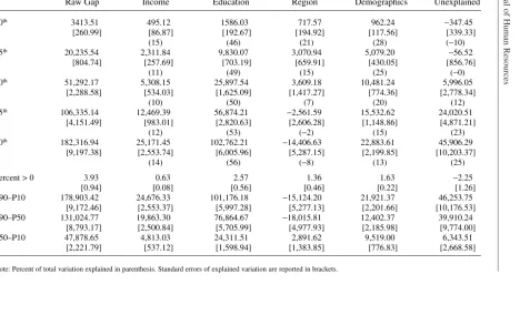
Consistent with previous evidence (Hao 2003), white households are wealthier than Mexican American households. The wealth gap between native-born Mexican American and white households is sizable, more than $51,000 at the median and more than $182,000 in the 90th percentile of the distribution. (See Table 2.) Not surpris-ingly, the wealth gap faced by households that have migrated from Mexico is even larger. For them the gap in median net worth is approximately $72,500, whereas the gap in households’ wealth at the 90th percentile approaches a quarter of a million dollars. (See Table 3.)
In both cases, most of the gap stems from differences in the current income levels and background characteristics of households, rather than from differences in the way in which—conditional on their incomes and characteristics—households have accu-mulated wealth in the past. At the median, for example, only 12 percent of native-born and 11 percent of foreign-born Mexican Americans’ wealth disadvantage is due to differences in these conditional wealth distributions themselves. Moreover, differ-ences in conditional wealth distributions lead the white/Mexican American gap in the proportion of families holding positive net worth to be smaller. These results are strik-ing in light of research suggeststrik-ing that relatively educated Mexican Americans have more present-oriented attitudes toward money and are less inclined to delay spending than are their white counterparts (Medina, Saegert, and Gresham 1996). Such differ-ences in attitudes are unaccounted for in our analysis and would be expected to increase the role of the conditional wealth distributions themselves in explaining the wealth gap. However, we find no evidence of such an effect and indeed for households at the bottom of the conditional wealth distribution, differences in wealth distributions narrow rather than widen the wealth gap.
Income disparities (conditional on education, location, and demographic characteris-tics) also explain relatively little of Mexican Americans’ wealth disadvantage, even at the top of the wealth distribution where the magnitude of the wealth gap is very large. While differences in conditional income distributions explain somewhat more of the wealth gap between foreign-born Mexican Americans and whites, it remains the case that as much or more of Mexican Americans’ relative wealth disadvantage is accounted for by differences in education and the demographic composition of households.
The Journal of Human Resources Table 2
Native-Born Mexican Americans to Whites
Raw Gap Income Education Region Demographics Unexplained
10th 3413.51 495.12 1586.03 717.57 962.24 −347.45
[260.99] [86.87] [192.67] [194.92] [117.56] [339.33]
(15) (46) (21) (28) (−10)
25th 20,235.54 2,311.84 9,830.07 3,070.94 5,079.20 −56.52
[804.74] [257.69] [703.19] [659.91] [430.05] [856.76]
(11) (49) (15) (25) (−0)
50th 51,292.17 5,308.15 25,897.54 3,609.18 10,481.24 5,996.05
[2,288.58] [534.03] [1,625.09] [1,417.27] [774.36] [2,778.34]
(10) (50) (7) (20) (12)
75th 106,335.14 12,469.39 56,874.21 −2,561.59 15,532.62 24,020.51
[4,151.49] [983.01] [2,820.63] [2,606.28] [1,148.86] [4,871.21]
(12) (53) (−2) (15) (23)
90th 182,316.94 25,171.45 102,762.21 −14,406.63 22,883.61 45,906.29
[9,197.38] [2,553.74] [6,005.96] [5,287.15] [2,199.85] [10,203.37]
(14) (56) (−8) (13) (25)
Percent > 0 3.93 0.63 2.57 1.36 1.63 −2.25
[0.94] [0.08] [0.56] [0.46] [0.22] [1.26]
P90–P10 178,903.42 24,676.33 101,176.18 −15,124.20 21,921.37 46,253.75
[9,172.46] [2,553.37] [5,997.28] [5,277.13] [2,201.66] [10,176.53]
P90–P50 131,024.77 19,863.30 76,864.67 −18,015.81 12,402.37 39,910.24
[8,793.17] [2,500.84] [5,705.99] [4,977.93] [2,185.98] [9,774.00]
P50–P10 47,878.65 4,813.03 24,311.51 2,891.62 9,519.00 6,343.51
[2,221.79] [537.12] [1,598.94] [1,383.85] [776.83] [2,668.58]
Cobb-Clark and Hildebrand
855
Raw Gap Income Education Region Demographics Unexplained
10th 3,873.33 1,800.18 1,018.43 648.31 1,659.23 −1,252.83
[289.84] [526.12] [997.90] [649.19] [605.32] [1,227.43]
(46) (26) (17) (43) (−32)
25th 24,891.31 7,102.42 8,031.86 1,627.87 8,131.55 −2.39
[381.90] [1,698.07] [2,919.05] [1,813.44] [1,604.12] [931.84]
(29) (32) (7) (33) (−0)
50th 72,428.81 15,135.36 27,406.05 −525.57 22,660.19 7,752.77
[836.53] [4,449.21] [6,333.45] [4,111.67] [4,556.04] [4,091.33]
(21) (38) (−1) (31) (11)
75th 142,171.55 27,406.28 73,605.93 −8,672.36 41,638.70 8,193
[2,629.32] [8,729.24] [12,735.06] [7,224.99] [7,438.28] [5,202.68]
(19) (52) (−6) (29) (6)
90th 249,484.00 50,441.34 140,917.36 −22,625.47 55,611.51 25,139.26
[6,493.06] [12,071.92] [24,633.59] [13,245.94] [13,961.15] [13,436.80]
(20) (56) (−9) (22) (10)
Percent > 0 10.95 4.69 4.18 1.68 5.31 −4.91
[1.06] [0.96] [3.17] [2.23] [2.05] [4.98]
P90–P10 245,610.67 48,641.15 139,898.92 −23,273.78 53,952.29 26,392.08
[6,480.08] [12,134.34] [24,768.28] [13,320.84] [14,037.66] [13,584.98]
P90–P50 177,055.19 35,305.97 113,511.30 −22,099.90 32,951.32 17,386.49
[6,287.40] [11,706.47] [24,769.82] [12,888.61] [14,338.91] [13,426.45]
P50–P10 68,555.48 13,335.18 26,387.62 −1,173.89 21,000.97 9,005.60
[785.44] [4,516.81] [6,291.77] [4,150.64] [4,537.72] [4,108.84]
less education. This relative lack of educational attainment contributes to producing a gap in net worth—even after controlling for differences in current income—that is quite large throughout the wealth distribution. Disparity in conditional education distributions explains up to two-thirds of the gap in the proportion of households with positive net worth and more than half the gap in the dispersion of net worth within the two popula-tions. These results are consistent with previous research documenting the strong, pos-itive relationship between education and wealth levels even when income is taken into account (see, Hurst, Luoh, and Stafford 1998; Altonji and Doraszelski 2005; Kapteyn, Alessie, and Lusardi 2005; Keister 2000; Amuedo-Dorantes and Pozo 2002) on the one hand and between education and the propensity to hold riskier, higher-return assets on the other (Chiteji and Stafford 1999; Rosen and Wu 2004).
Differences in the demographic composition—in particular, in the age of the house-hold head and the number of children present—also contribute to significantly widen-ing the wealth gap, particularly for foreign-born Mexican Americans. At the median, fully 20 percent of native-born and 31 percent of foreign-born Mexican Americans’ wealth disadvantage is attributable to the fact that these households have more young children and heads who are younger. In both cases, the wealth gap stemming from dif-ferences in demographic characteristics is larger in magnitude than that stemming from differences in conditional income distributions. Demographic characteristics are also important in explaining the wider dispersion of wealth amongst white households.
Finally, the differential in geographic concentration plays a much smaller role than these other factors in generating the wealth gap between Mexican Americans and non-Hispanic whites. At the same time, it is interesting that for both native-born and foreign-born Mexican Americans geographic concentration serves to widen the gap in net worth at the bottom of the wealth distribution, but narrow it at the top of the wealth distribution leading to a narrowing of the relative wealth dispersion. This may suggest that geographic clustering in states such as California benefits those wealthier Mexican Americans who can access the relatively expensive homeownership market, but is detrimental to those who cannot.
B. Mexican Americans versus Blacks
The wealth gap between native-born Mexican Americans and blacks is negative (though relatively small and occasionally insignificant) throughout the entire wealth distribution, indicating that Mexican American households hold higher levels of net worth than do black households. (See Table 4.) Differences in conditional wealth dis-tributions more than account for the lower net worth of black households. We calcu-late, for example, that if black households had the same conditional income, education, and geographic distributions and the same demographic characteristics as native-born Mexican American households, they would have a wealth disadvantage of $11,217 at the median. In short, differences in conditional wealth distributions imply that black households hold substantially less wealth than otherwise similar native-born Mexican American households.
Cobb-Clark and Hildebrand
857
Raw Gap Income Education Region Demographics Unexplained
10th −338.80 −29.57 20.82 −346.78 84.92 −68.2
[264.11] [82.40] [163.28] [265.00] [156.42] [357.33]
(9) (−6) (102) (−25) (20)
25th −1,893.84 −374.71 1,181.46 −919.43 844.55 −2,625.71
[810.98] [143.63] [337.28] [525.28] [233.53] [898.58]
(20) (−62) (49) (−45) (139)
50th −4,343.87 −1,451.56 7,406.85 −3,605.94 4,524.26 −11,217.48
[2,502.87] [525.79] [1,630.84] [2,493.85] [946.57] [3,939.64]
(33) (−171) (83) (−104) (258)
75th −10,582.30 −1,784.87 13,801.98 −11,987.51 4,634.89 −15,246.79
[4,352.20] [761.46] [2,530.79] [3,531.72] [1,260.88] [5,647.26]
(17) (−130) (113) (−44) (144)
90th −36,200.05 −2,736.58 26,985.92 −13,232.02 5,661.13 −52,878.49
[9,448.61] [1,645.53] [3,960.36] [5,528.85] [2,244.32] [11,246.32]
(8) (−75) (37) (−16) (146)
Percent > 0 −3.47 −0.54 1.56 −3.66 1.28 −2.11
[1.10] [0.12] [0.78] [1.27] [0.36] [1.65]
P90–P10 −35,861.25 −2,707.02 26,965.09 −12,885.24 5,576.21 −52,810.29
[9,423.55] [1,646.98] [3,966.10] [5,516.76] [2,245.61] [11,225.14]
P90–P50 −31,856.19 −1,285.03 19,579.06 −9,626.08 1,136.87 −41,661.01
[9,007.25] [1,655.30] [4,021.47] [5,414.75] [2,315.55] [1,0851.50]
P50–P10 −4,005.06 −1,421.99 7,386.03 −3,259.16 4,439.34 −11,149.29
[2,436.75] [529.69] [1,624.33] [2,435.23] [950.86] [3,879.17]
The Journal of Human Resources Table 5
Foreign-Born Mexican Americans to Blacks
Raw Gap Income Education Region Demographics Unexplained
10th 121.01 158.71 −551.51 −376.82 499.03 391.61
[277.66] [220.45] [466.83] [395.67] [280.26] [366.71]
(131) (−456) (−311) (412) (324)
25th 2,761.93 1,250.58 950.73 −1,503.84 1,177.13 887.33
[308.00] [448.67] [849.39] [800.85] [492.29] [1,000.15]
(45) (34) (−54) (43) (32)
50th 16,792.77 2,651.72 11,079.74 −4,571.42 10,209.51 −2,576.78
[1,223.89] [1,650.25] [4,686.15] [4,728.45] [2,941.79] [63,07.05]
(16) (66) (−27) (61) (−15)
75th 25,254.11 5,349.02 24,775.14 −17,874.25 15,419.03 −2,414.83
[2,818.59] [3,553.79] [8,240.18] [7,206.07] [4,987.22] [9,861.40]
(21) (98) (−71) (61) (−10)
90th 30,967.01 10,826.49 49,111.95 −20,797.55 17,091.57 −25,265.45
[6,442.38] [4,071.54] [9,319.82] [8,762.56] [6,194.09] [9,351.85]
(35) (159) (−67) (55) (−82)
Percent > 0 3.54 2.45 4.70 −9.77 3.19 2.97
[1.20] [0.93] [5.20] [3.92] [2.09] [3.39]
P90–P10 30,846.00 10,667.78 49,663.46 −20,420.72 16,592.55 −25,657.07
[6,405.84] [4,117.00] [9,350.57] [8,777.08] [6,198.15] [9,395.76]
P90–P50 14,174.24 8,174.77 38,032.21 −16,226.13 6,882.06 −22,688.67
[6,240.25] [4,196.62] [9,057.43] [9,402.65] [6,813.86] [10,778.48]
P50–P10 16,671.76 2,493.01 11,631.25 −4,194.59 9,710.48 −2,968.39
[1,170.22] [1,668.45] [4,689.98] [4,714.44] [2,913.88] [6,297.56]
of foreign-born Mexican Americans by substantially narrowing the median wealth gap. These effects are generally not significant, however.
Examination of our dispersion measures indicates that net worth is more unequally distributed amongst native-born Mexican American households than amongst black households particularly in the top half of the distribution. Divergences in conditional wealth distributions more than explain the higher wealth disparity amongst native-born Mexican Americans. Although the gap in wealth dispersion is positive in the case of foreign-born Mexican American and black households, here too disparity in conditional wealth distributions serves to increase the wealth inequality of Mexican Americans relative to blacks.
Consistent with results for white households, differences in the conditional educa-tion distribueduca-tions and in the distribueduca-tion of demographic characteristics each lead black households to have a net worth advantage over native-born Mexican American house-holds which would be—in isolation—large enough to completely overcome the observed negative gap in median wealth. For example, at the median, differences in the conditional education distributions lead black households to have a net worth level that is $7,407 higher than that of native-born Mexican Americans, while differences in the age composition of households generate a wealth advantage of $4,524. Education dif-ferences between the two groups are important in increasing the wealth dispersion of blacks relative to native-born Mexican Americans. Similar results are observed for for-eign-born Mexican Americans and it is interesting that this occurs despite other evi-dence that by age 24 there is more variation in educational attainment amongst Hispanic men as a whole than amongst black men (Cameron and Heckman 2001). All in all, differences in education have a direct and important effect in diminishing the relative wealth position of Mexican Americans.
Disparity in the income levels of blacks and Mexican Americans (conditional on geo-graphic distribution and household composition) worsens the relative wealth position of foreign-born Mexican Americans, but improves the wealth position of native-born house-holds slightly though these effects are not always significant. Specifically, everything else equal, at the median differences in the conditional income distributions would lead to blacks holding approximately $1,452 less wealth than similar Mexican Americans. This effect, though small and significant implies that conditional on their characteristics native-born Mexican Americans have more income than otherwise similar blacks.
Finally, the geographic concentration of wealthier, native-born Mexican American households leads to a substantial improvement in their net worth position relative to black households. This effect is striking in both its magnitude and consistency. For example, at the 90th percentile of the wealth distribution, differences in conditional geographic distributions give native-born Mexican Americans a wealth advantage of approximately $13,000. For many foreign-born and less wealthy Mexican Americans disparity in geographic concentration has no significant effect on the overall wealth gap. Thus, while geographic concentration works to the disadvantage of poorer Mexican Americans relative to poorer non-Hispanic white households, this is not the case when our focus is on black households.
C. Native-Born versus Foreign-Born Mexican Americans
The Journal of Human Resources Table 6
Foreign- to Native-Born Mexican Americans
Raw Gap Income Education Region Demographics Unexplained
10th 459.81 91.81 −6.24 −34.81 48.15 360.91
[305.58] [292.54] [327.10] [217.04] [256.21] [443.09]
(20) (−1) (−8) (10) (78)
25th 4,655.77 1,637.59 123.65 62.77 1,413.60 1,418.16
[738.33] [512.83] [711.54] [436.31] [587.38] [780.04]
(35) (3) (1) (30) (30)
50th 21,136.64 4,588.19 5,098.34 −763.79 6,387.94 5,825.96
[2,320.86] [2,010.00] [3,334.41] [1,913.48] [2,410.71] [3,617.54]
(22) (24) (−4) (30) (28)
75th 35,836.41 10,522.37 9,224.95 −7,549.76 11,569.49 12,069.35
[4,529.35] [3,901.29] [5,885.91] [3,815.28] [4,251.71] [7,405.46]
(29) (26) (−21) (32) (34)
90th 67,167.06 23,032.65 30,619.20 −11,955.83 29,685.14 −4,214.1
[10,707.90] [8,475.43] [11,955.40] [8,246.25] [9,770.97] [11,641.98]
(34) (46) (−18) (44) (−6)
Percent > 0 7.02 1.69 1.18 −0.97 0.44 4.67
[1.41] [0.77] [1.68] [0.93] [1.09] [2.41]
P90–P10 66,707.25 22,940.84 30,625.44 −11,921.01 29,636.99 −4,575.00
[10,682.94] [8,475.20] [11,941.15] [8,252.96] [9,767.15] [11,634.65]
P90–P50 46,030.42 18,444.46 25,520.86 −11,192.04 23,297.20 −10,040.06
[10,194.18] [8,568.71] [11,353.26] [8,214.67] [9,716.26] [11,018.90]
P50–P10 2,0676.82 4,496.38 5,104.58 −728.98 6,339.79 5,465.06
[2,279.44] [2,001.97] [3,323.70] [1,907.66] [2,405.18] [3,621.99]
because it allows us to focus specifically on the role of nativity holding ethnic origin constant. At the median, native-born Mexican Americans have just over $21,000 more in net worth than their foreign-born counterparts. Most of this nativity gap in median wealth can be explained by differences in the income and background characteristics of households, with differences in the conditional wealth distributions of the two groups having an insignificant effect on the wealth gap. This result is somewhat surprising in light of the different incentives that foreign- and native-born Mexican Americans may have to accumulate U.S.-specific net worth. For example, Amuedo-Dorantes and Pozo (2002) conclude that many Mexican migrants use remittances to insure against risky labor earnings. Unfortunately, standard wealth data sets such as the SIPP do not contain information about household remittances and our inability to account for this would be expected to drive a wedge between the conditional wealth distributions of native-born and foreign-born Mexican Americans. We do not see any evidence of this, however.
Not surprisingly, income differences are a key factor in producing the nativity wealth gap. Disparities in current household income explain, for example, 22 percent of the overall wealth gap at the median, an effect that is roughly the same throughout the distribution. Education differences between native-born and foreign-born Mexican Americans also contribute to the wealth gap, though the magnitude of the education effect varies substantially across the different deciles of the wealth distri-bution and—unlike the previous cases—is often insignificant.
What is more striking is the importance of households’ demographic composition in understanding wealth differentials between foreign- and native-born Mexican Americans. Fully, 30 percent—the largest share—of the wealth gap is attributable to differences in the age of the head and the numbers of children under the age of 18 living in the household at the median. The effect of demographic characteristics becomes increasingly important as one moves up the wealth distribution, accounting for almost half the gap in the 90th percentile. Thus, foreign-born Mexican Americans have less wealth than their native-born counterparts in large part because they are younger and have more young children.
Finally, although relative to their native-born counterparts, foreign-born Mexican Americans are more likely to live in California rather than Texas, this geographic con-centration has no significant effect on the relative wealth position of the two groups.
D. Robustness Testing: The Role of Permanent Income
Our results are striking in that current income—while important—typically is less important than education in explaining the wealth gap between Mexican Americans and other groups. One possible interpretation of these results is that current income is simply less important than permanent income in explaining wealth. After all, life cycle theory suggests that it is the permanent component of income upon which sav-ings and consumption decisions—and ultimately wealth accumulation—are based. Similarly, the relatively large education effect might arise because education is more closely related to permanent rather than current income. Since we do not take perma-nent income into account, some of the education effect we are measuring might be attributable to a permanent income effect.
used predicted income as a proxy for permanent income when estimating wealth equations (Cobb-Clark and Hildebrand 2006a). Here, using factors such as age, edu-cation, geographic loedu-cation, etc. to predict income tends to confound the interpreta-tion of the decomposiinterpreta-tion itself. Consequently, we have chosen to present decompositions based on current household income. At the same time, if predicted income is a reasonable proxy for permanent income then replicating the decomposi-tion analysis using a predicted income measure can shed light on the extent to which the effect of the education component might be overstated and the income component understated because of the omission of a permanent income measure.
We find that using predicted rather than current income has very little effect on the magnitude of the education-related wealth disadvantage that Mexican Americans face relative to blacks or whites.11At the median, the education component for native-born
Mexican Americans relative to blacks falls from—171 percent of the gap (Table 4) to—160 percent of the gap. In all other cases, the proportion of the wealth gap due to education is much the same or even slightly larger when we account for predicted income. These results are inconsistent with the hypothesis that the education compo-nent largely reflects permacompo-nent income differences not accounted for by the current income measure. Moreover, although the share of the wealth gap between foreign-born Mexican Americans and whites that is explained by income differences increases when we control for predicted rather than current income, in general the income com-ponent of the Mexican American wealth gap is generally smaller at the median when we consider predicted income.
Thus, it does not seem to be the case that a permanent income story completely explains the large role of education in explaining the relative wealth position of Mexican Americans. In all cases, the results using the two-income measures are remarkably consistent and there remains a large direct role for education in producing wealth gaps even when we consider predicted rather than current income. This is per-haps not surprising given the direct role that education plays in driving wealth levels (see Hurst, Luoh, and Stafford 1998; Altonji and Doraszelski 2005; Kapteyn, Alessie, and Lusardi 2005; Amuedo-Dorantes and Pozo 2002) and portfolio allocations (Chiteji and Stafford 1999) even when permanent income is controlled for.
E. Comparing Ethnic and Racial Wealth Gaps
Although the wealth position of Mexican Americans has received little attention, the vast disparities in the wealth of black and white families has been the focus of recent debate with attention centered primarily on assessing the extent to which observable dif-ferences in the income streams, human capital endowments, and demographic compo-sition of households explain the racial wealth gap. (See Blau and Graham 1990; Gittleman and Wolff 2000; Altonji and Doraszelski 2005; Barsky et al. 2002.) In most cases, researchers have employed standard Oaxaca-Blinder techniques to decompose relative mean wealth levels, though Barsky et al. (2002) are a recent exception. A brief
review of this literature suggests that the capacity of observed characteristics to explain relative wealth levels depends fundamentally on the specific decomposition used. Parametric decompositions using the conditional wealth distribution of whites weighted by the characteristics of blacks to generate counterfactual distributions indicate that the disparity in observed characteristics explains between 70 and 80 percent of the mean racial wealth gap (see Blau and Graham 1990; Gittleman and Wolff 2000; and Altonji and Doraszelski 2005), while nonparametric methods suggest that 64 percent of the mean racial wealth gap is explained by relative earnings (Barsky et al. 2002).
To place our results for Mexican Americans in context, we also used our data sample and the methods outlined in Section IIIA to decompose the racial wealth gap. As approx-imately 98 percent of the native-born and foreign-born Mexican Americans in our sam-ple identify themselves as white, this comparison allows us to separately consider the effects of ethnicity on the one hand and race on the other in producing wealth gaps. The results (see Appendix 1 Table A1) indicate that—unlike the case for the ethnic wealth gap—the majority of the racial wealth gap is attributable to divergence in conditional wealth distributions. At the median, for example, fully 55 percent of the wealth gap between white and black families is unexplained by differences in income, education, geographic distribution, and demographics. The relative wealth position of white and black families stems largely from differences in they way in which—conditional on their characteristics—wealth is accumulated. In contrast, only 12 (11) percent of the median wealth gap between native-born (foreign-born) Mexican Americans and whites remains unexplained by these same characteristics (see Tables 2 and 3). The ethnic wealth gap— unlike the racial wealth gap—is almost completely attributable to differences in the income, family structure, educational attainment, and geographic distribution of families.
V. Conclusion
Racial and ethnic disparities in wealth levels are much larger than cor-responding disparities in income levels. Yet despite decades of research directed toward understanding the processes that give rise to racial and ethnic income differ-entials, we know relatively little about how these income differentials are in turn reflected in the immense wealth disparities between groups. Taxing data requirements and the inherent complexities in the underlying earnings, savings, and consumption decisions that form the wealth accumulation process have traditionally made it diffi-cult to advance our understanding of the causes of racial and ethnic wealth disparities. This is unfortunate because wealth provides the resources necessary to maintain con-sumption levels in the face of economic hardship and consequently is an important measure of overall economic well-being.
more children and heads who are younger. Similarly, low educational attainment amongst Mexican Americans has a direct effect in producing a wealth gap relative to other groups even after differences in income are taken into account though education does not significantly affect the nativity wealth gap. Mexican Americans’ relative wealth disadvantage is in large part not the result of differences in the way in which households—conditional on their characteristics—accumulate net worth. Similarly, income differences, while important, are generally not the key factor driving relative wealth positions.
Cobb-Clark and Hildebrand
865
Raw Gap Income Education Region Demographics Unexplained
10th 3,752.32 813.38 1,113.90 253.64 376.06 1,195.34
[218.47] [59.00] [76.28] [70.58] [41.85] [181.44]
(22) (30) (7) (10) (32)
25th 22,129.38 2,955.14 4,678.56 1,774.92 1,626.00 11,094.76
[463.73] [133.52] [185.04] [201.63] [108.32] [440.13]
(13) (21) (8) (7) (50)
50th 55,636.03 5,663.57 10,640.86 5,409.90 3,164.84 30,756.87
[1,188.74] [238.15] [333.98] [371.28] [183.62] [1,200.25]
(10) (19) (10) (6) (55)
75th 116,917.44 12,203.03 23,610.35 11,143.61 5,016.20 64,944.24
[1,973.77] [535.62] [711.70] [744.41] [336.11] [1,833.14]
(10) (20) (10) (4) (56)
90th 218,516.99 21,948.37 40,960.32 16,209.80 7,054.27 132,344.23
[3,525.09] [1,208.57] [1,547.33] [1,492.68] [698.57] [3,263.10]
(10) (19) (7) (3) (61)
Percent > 0 7.41 0.65 0.76 0.19 0.35 5.46
[0.55] [0.03] [0.06] [0.08] [0.03] [0.57]
P90–P10 214,764.67 21,134.99 39,846.41 15,956.17 6,678.21 131,148.89
[3,520.29] [1,209.64] [1,545.39] [1,488.24] [699.10] [3,250.75]
P90–P50 162,880.95 16,284.80 30,319.46 10,799.91 3,889.43 101,587.36
[3,397.05] [1,191.19] [1,533.60] [1,439.50] [708.92] [3,126.61]
P50–P10 51,883.72 4,850.19 9,526.96 5,156.26 2,788.78 29,561.53
[1,142.55] [243.69] [334.67] [357.57] [183.75] [1,158.71]
References
Joseph G. Altonji, and Ulrich Doraszelski. 2005. “The Role of Permanent Income and Demographics in Black/White Differences in Wealth.” Journal of Human Resources
40(1):1–30.
Amuedo-Dorantes, Catalina, and Susan Pozo. 2002. “Precautionary Savings by Young Immigrants and Young Natives.” Southern Economic Journal69(1):48–71.
Bahizi, Pierre. 2003. “Retirement Expenditures for Whites, Blacks, and Persons of Hispanic Origin.” Monthly Labor Review126(6):20–22.
Barsky Robert, John Bound, Kerwin Charles, and Joseph P. Lupton. 2002. “Accounting for the Black-White Wealth Gap: a Nonparametric Approach.” Journal of the American Statistical Association97(459):663–73.
Bertaut, Carol, and Martha Starr-McCluer. 1999. “Household Portfolios in the United States.” Working Paper, Federal Reserve Board of Governors, November 30, 1999.
Blau, Francine D., and John W. Graham. 1990. “Black-White Differences in Wealth and Asset Composition.” Quarterly Journal of Economics105(2):321–39.
Blinder, Alan S. 1973. “Wage Discrimination: Reduced Form and Structural Estimation.”
Journal of Human Resources8(4):436–55.
Georges J. Borjas. 2002. “Homeownership in the Immigrant Population.” Journal of Urban Economics3(52):448–76.
Butcher, Kristin F., and John DiNardo. 2002. “The Immigrant and Native-Born Wage Distributions: Evidence from United States Censuses.” Industrial and Labor Relations Review56(1):97–121.
Cameron, Stephen V., and James J. Heckman. 2001. “The Dynamics of Educational Attainment for Black, Hispanic, and White Males.” Journal of Political Economy
109(3):455–99.
Charles, Kerwin K., and Erik Hurst. 2003. “The Correlation of Wealth Across Generations.”
Journal of Political Economy111(6):1155–82.
Chiteji, Ngina S., and Frank P. Stafford. 1999. “Portfolio Choices of Parents and Their Children as Young Adults: Asset Accumulation by African-American Families.” American Economic Review89(2):377–80.
Choudhury, Sharmila. 2001. “Racial and Ethnic Differences in Wealth and Asset Choices.”
Social Security Bulletin64(4):1–15.
Cobb-Clark, Deborah A., and Vincent A. Hildebrand. 2006a. “The Wealth and Asset Holdings of U.S.-Born and Foreign-Born Households.” Review of Income and Wealth52(1):17–42. ———. 2006b. “The Portfolio Choices of Hispanic Couples.” Social Science Quarterly.
Forthcoming.
Cotton, Jeremiah. 1988. “On the Decomposition of Wage Differentials.” Review of Economics and Statistics70(2):236–43.
DiNardo, John, Nicole M. Fortin, and Thomas Lemieux. 1996. “Labor Market Institutions and the Distribution of Wages, 1973–1992: A Semiparametric Approach” Econometrica
64:1001–1044.
Fairlie, Robert W., and Christopher Woodruff. 2005. “Mexican American Entrepreneurship.” University of California, Santa Cruz. Unpublished.
Gittleman, Maury, and Edward N. Wolff. 2000. “Racial Wealth Disparities: Is the Gap Closing?” Levy Economics Institute Working Paper No. 311.
Greene, William H. 1997. Third Edition Econometric Analysis. New Jersey: Prentice Hall. Grogger, Jeffrey, and Stephen J. Trejo. 2002. Falling Behind or Moving Up? The
Intergenerational Progress of Mexican Americans, Public Policy Institute of California: San Francisco, Calif..
Hao, Lingxin. 2003. “Immigration and Wealth Inequality in the U.S.” Russell Sage Foundation Working Paper #202.
Hurst, Erik, Ming Ching Luoh, and Frank Stafford. 1998. “The Wealth Dynamics of
American Families, 1984–94.” Brookings Papers on Economic Activity1: 267–337.
Hyslop, Dean R., and David C. Maré 2003, “Understanding New Zealand’s Changing Income Distribution 1983–1998: A Semiparametric Analysis.” July 2003. Unpublished.
Juster, F. Thomas, and Kathleen A. Kuester. 1991. “Differences in the Measurement of Wealth, Wealth Inequality, and Wealth Composition Obtained from Alternative U.S.
Surveys.” Review of Income and Wealth37(1):33–62.
Juster, F. Thomas, James P. Smith, and Frank Stafford. 1999. “The Measurement and
Structure of Household Wealth.” Labour Economics6:253–75.
Kapteyn, Arie, Rob Alessie, and Annamaria Lusardi. 2005. “Explaining the Wealth Holdings
of Different Cohorts: Productivity Growth and Social Security”. European Economic
Review49(5):1361–91.
Keister, Lisa A. 2000. “Family Structure, Race, and Wealth Ownership: A Longitudinal Exploration of Wealth Accumulation Processes.” Department of Sociology, Ohio State University. Unpublished.
Medina, José F., Joel Saegert, and Alicia Gresham. 1996. “Comparison of Mexican-American
and Anglo-American Attitudes Toward Money.” Journal of Consumer Affairs30(1):124–45.
Menchik, Paul L. and Nancy Ammon Jianakoplos. 1997. “Black-White Wealth Inequality: Is
Inheritance the Reason.” Economic Inquiry3(2):428–42.
Oaxaca, Ronald. 1973. “Male-Female Wage Differentials in Urban Labour Markets.”
International Economic Review14:693–709
Osili, Una Okonkwo and Anna Paulson. 2003. “The Financial Assimilation of Immigrants in the U.S.” Unpublished.
Paulin, Geoffrey D. 2003. “A Changing Market: Expenditures by Hispanic Consumers,
Revisited.” Monthly Labor Review126(8):12–35.
Reimers, Cordelia W. 1984. “Sources of Family Income Differentials Among Hispanics,
Blacks, and White Non-Hispanics.” The American Journal of Sociology89(4): 889–903.
Rosen, Harvey S. and Stephen Wu. 2004. “Portfolio Choice and Health Status.” Journal of
Financial Economics2(3):457–84.
Shorrocks, Anthony F. 1999. “Decomposition Procedures for Distributional Analysis: A United Framework Based on the Shapley Value.” University of Essex, June 1999. Unpublished.
Skerry, Peter. 2000. Counting on the Census? Race, Group Identity, and the Evasion of
Politics. Washington, DC: The Brookings Institute.
Smith, James P. 1995. “Racial and Ethnic Differentials in Wealth in the HRS.” Journal of
Human Resources30(Supplement): S158–S183.
Trejo, Stephen J. 1997. “Why Do Mexican Americans Earn Low Wages?” Journal of Political
Economy105(6):1235–68.
U.S. Bureau of the Census, Economics and Statistics Administration. 1995. The Nation’s
Hispanic Population—1994, Statistical Brief, SB/95-25, September 1995. Washington, D.C.: GPO.
U.S. Bureau of the Census, Economics and Statistics Administration. 2001a. The Hispanic
Population in the United States: Census 2000 Brief, Current Population Reports, P20–535, (by Melissa Therrien and Roberto R. Ramirez), March 2001. Washington, D.C.: GPO.
U.S. Bureau of the Census, Economics and Statistics Administration, 2001b. The Hispanic
Population: Census 2000 Brief, (by Betsy Guzma’n), May 2001. Washington, D.C.: GPO U.S. Immigration and Naturalization Service (USINS). 2002. Statistical Yearbook of the
Immigration and Naturalization Service, 2000, September 2002. Washington, D.C.: GPO. Wakita, Satomi, Vicki Schram Fitzsimmons, and Tim Futing Liao, 2000. “Wealth:
Determinants of Savings Net Worth and Housing Net Worth of Pre-Retired Households.”