Stacy Dale is an Associate Director and Senior Researcher at Mathematica Policy Research, Princeton, New Jersey. Alan Krueger is the Bendheim Professor of Economics and Public Affairs at Princeton Univer-sity. The authors thank the Mellon Foundation for fi nancial support; Ed Freeland for obtaining permission of participating colleges; Matthew Jacobus and Licia Gaber Baylis for skilled computer programming sup-port; Mike Risha of SSA for merging the C&B data with SSA data and for tirelessly running our programs; Matt Chingos, Jesse Rothstein, Lawrence Katz, Sarah Turner, and Mark Dynarski for helpful comments; Mark Long for providing data on college SAT scores; and several anonymous reviewers for insightful suggestions.
Researchers may apply to the Andrew W. Mellon Foundation to acquire the College and Beyond data used in this paper. The authors of this paper are willing to provide guidance on the application process.
[Submitted May 2012; accepted May 2013]
ISSN 0022- 166X E- ISSN 1548- 8004 © 2014 by the Board of Regents of the University of Wisconsin System
Estimating the Effects of College
Characteristics over the Career Using
Administrative Earnings Data
Stacy B. Dale
Alan B. Krueger
A B S T R A C T
We estimate the labor market effect of attending a highly selective college, using the College and Beyond Survey linked to Social Security Administration data. We extend earlier work by estimating effects for students that entered college in 1976 over a longer time horizon (from 1983 through 2007) and for a more recent cohort (1989). For both cohorts, the effects of college characteristics on earnings are sizeable (and similar in magnitude) in standard regression models. In selection- adjusted models, these effects generally fall to close to zero; however, these effects remain large for certain subgroups, such as for black and Hispanic students.
I. Introduction
Students who attend higher- quality colleges earn more on average than those who attend colleges of lesser quality. However, it is unclear why this dif-ferential occurs. Do students who attend more selective schools learn skills that make them more productive workers, as would be suggested by human capital theory? Or, consistent with signaling models, do higher- ability students—who are likely to be-come more productive workers—attend more selective colleges?
earn-ings is crucial for parents deciding where to send their children to college, for col-leges selecting students, and for policymakers deciding whether to invest additional resources in higher- quality institutions. However, obtaining unbiased estimates of the effects of college characteristics is diffi cult because of unobserved characteristics that affect both a student’s attendance at a highly selective college and his or her later earnings. In particular, the same characteristics (such as ambition) that lead students to apply to highly selective colleges may also be rewarded in the labor market. Like-wise, the attributes that admissions offi cers are looking for when selecting students for college may be similar to the attributes that employers are seeking when hiring and promoting workers.
A wide literature exists on the labor market effects of college characteristics, as summarized in Hoxby (2009) and Hershbein (2013). Many papers have used regres-sion models to control for observed student characteristics, such as high school grades, standardized test scores, and parental background (see, for example, Monks 2000; Brewer and Ehrenberg 1996; Black and Smith 2004), and generally fi nd that attend-ing a higher- quality college is associated with higher earnattend-ings. However, studies that attempt to adjust for unobserved student quality have reported mixed fi ndings. Dale and Krueger (2002) fi nd that the effect of college characteristics falls substantially after implementing their selection- correction, which partially adjusts for unobserved student quality by controlling for the average student SAT score of the colleges that students apply to and are accepted or rejected by. Hoekstra (2009) uses a regression discontinuity design that compares the earnings of students who were just above the admissions cutoff for a state university to those that were just below it; he fi nds that at-tending the fl agship state university results in 20 percent higher earnings 5 to 10 years after graduation for white men, but he does not fi nd an effect on earnings for white women. Using an instrumental variables strategy, Long (2008) did not fi nd a consistent relationship between college characteristics and earnings. Lindahl and Regner (2005) use sibling data to illustrate that the effect of college quality might be overstated if family characteristics are not fully adjusted for because cross- sectional estimates are twice as large as within- family estimates. It is important to note that most of the above literature has used a single college characteristic—such as school average SAT score, expenditures per student, the Barron’s index, or whether the student attended a fl agship state university—as a proxy for college quality. However, Black and Smith (2006) show that the estimates of the effects of school quality are attenuated when a single measure is used; the effects of composite measures are higher.
One recent study (Hershbein 2013) has tried to distinguish between human capital models and signaling models by assessing how the relationship between grade point average (GPA), college selectivity, and wages changes over time. He fi nds that the return to GPA is smaller at more selective schools than at less selective schools, which is consistent with signaling models. (The marginal benefi t of information about GPA is lower at more selective schools because attending a highly selective college already sends a signal about student ability).
Dale and Krueger 325
Katz and Murphy 1992). However, Black, Daniel, and Smith (2005) show that the effects of college quality for a single cohort—the 1979 cohort of the National Longi-tudinal Survey of Youth (NLSY)—remain stable over an 11- year horizon.
Little research has examined the effects of college characteristics for recent cohorts. This is a notable gap in the literature; one might expect that it would be more impor-tant for students who entered college recently to distinguish themselves by attending more selective colleges because the percentage of students enrolling in college has increased.1 Those studies that do use recent cohorts tend to model earnings early in the career. For example, Long (2008, 2009) used a relatively recent cohort (the 1992 cohort of the National Education Longitudinal Study [NELS]), but he was only able to examine the earnings of students relatively early in their careers when they were only 26 years old.
In this paper, we examine whether the college that students attend (within a set of somewhat selective to highly selective colleges) affects their later earnings. This paper replicates earlier work that examined the relationship between the college that students attended in 1976 and the earnings they reported in 1995 in the College and Beyond (C&B) followup survey (Dale and Krueger 2002); it also extends this earlier work in important respects. First, we estimate the effects of several college characteristics that are commonly used as proxies for college quality (college average SAT score, the Bar-ron’s index, and net tuition) for a recent cohort of students—those who entered college in 1989. By linking the C&B data to administrative records from the Social Security Administration (SSA), we are able to follow this cohort for 18 years after the students entered (and 14 years after they likely would have graduated from) college. Second, we estimate the return to college characteristics for the 1976 cohort over a long time horizon, from 1983 to 2007. Because we use administrative earnings records from tax data, our earnings measure is presumably more reliable than much of the prior literature, which is generally based on self- reported earnings. The use of administra-tive earnings data allows us to follow a recent cohort of students over a longer period of time than is possible in many of the longitudinal databases that are typically used to study the returns to college characteristics. For example, the NELS, High School and Beyond, and the National Longitudinal Study of the High School Class of 1972 (NLS- 72) only follow students for 6 to 10 years after they would have likely graduated from college; although the NLSY follows students for a longer period of time, students from the relatively recent cohort (who were ages 12 to 16 in 1997) are now too early in their post- collegiate careers to generate meaningful estimates of the labor market effects of college characteristics.
As in the rest of the literature, we fi nd that the effect of each college characteristic is sizeable for both cohorts in cross- sectional least squares regression models that control for variables commonly observed by researchers (such as student character-istics and SAT scores). However, when we adjust for a proxy for unobserved student characteristics—namely, by controlling for the average SAT score of the colleges that students applied to—our estimates for the effects of college characteristics fall sub-stantially and are generally indistinguishable from zero for both the 1976 and 1989
cohort of students. Notable exceptions are for racial and ethnic minorities (black and Hispanic students) and for students whose parents have relatively little education; for these subgroups, our estimates remain large, even in models that adjust for unob-served student characteristics. One possible explanation for this pattern of results is that highly selective colleges provide access to networks for minority students and for students from disadvantaged family backgrounds that are otherwise not available to them. Finally, contrary to expectations, our estimates do not suggest that the effects of college characteristics (within the set of C&B schools) increased for students who entered college more recently because estimates for the 1976 and 1989 cohort are similar when we compare the estimates for each cohort at a similar stage relative to college entry (approximately 18 to 19 years after the students entered college).
II. Methods
The college application process involves a series of choices. First, students choose where to apply to college; then, colleges decide which students to admit. Finally, students choose which college to attend from among the set of schools to which they were admitted. The diffi culty with estimating the labor market return to college quality is that not all of the characteristics that lead students to apply to and attend selective colleges are observed by researchers, and unobserved student charac-teristics are likely to be positively correlated with both school quality and earnings.
We assume the equation relating earnings to the students’ attributes is (1) ln Wi = β0 + β1Qi + β2X1i + β3X2i + εi,
where Q is a measure of the selectivity of the college student i attended, X1 and X2 are two sets of characteristics that affect earnings, and εi is an idiosyncratic error term that is uncorrelated with the other explanatory variables in Equation 1. X1 is a vector that includes variables that are observable to researchers, such as grades and SAT scores, whereas X2 is a vector that includes variables that are not observable to researchers, such as student motivation and creativity (that are at least partly revealed to admissions offi cers through detailed transcript information, essays, interviews, and recommendations). Both X1 and X2 affect the set of colleges that students apply to, whether they are admitted, and possibly which school they attend. The parameter β1
represents the gross monetary payoff to attending a more selective college. Early lit-erature on the returns to school quality was generally based on a wage equation that omitted X2:
(2) ln Wi = ′0+ ′1Qi + ′2X1i+ ui.
dimen-Dale and Krueger 327
sions in X2 and Q, and these same dimensions are likely to be positively correlated, the coeffi cient on school quality will be biased upward.
To address the selection problem, we use one of the selection- adjusted models— referred to as the “self- revelation model”—in Dale and Krueger (2002). This model assumes that students signal their potential ability, motivation, and ambition by the choice of schools they apply to. If students with greater unobserved earnings potential are more likely to apply to more selective colleges, the error term in Equation 2 could be modeled as a function of the average SAT score (denoted AVG) of the schools to which the student applied: ui = t0 + t1AVGi + vi. If vi is uncorrelated with the SAT score of the school the student attended, one can solve the selection problem by including AVG in the wage equation. This approach is called the self- revelation model because individuals reveal their unobserved characteristics by their college application behav-ior. This model also includes dummy variables indicating the number of schools the students applied to (in addition to the average SAT score of the schools) because the number of applications a student submits may also reveal unobserved student traits such as persistence.
Dale and Krueger (2002) also estimated a matched applicant model that included an unrestricted set of dummy variables indicating groups of students who received the same admissions decisions (that is, the same combination of acceptances and rejec-tions) from the same set of colleges. The self- revelation model is a special case of the matched applicant model. The matched applicant model and self- revelation model yielded coeffi cients that were similar in size, but the self- revelation model yielded smaller standard errors. Because of the smaller sample size in the present analysis, we therefore focus on the self- revelation model.
As discussed in more detail Dale and Krueger (2002), a critical assumption of the self- revelation model is that students’ enrollment decisions are uncorrelated with the error term of Equation 2 and X2. Our selection correction provides an unbiased esti-mate of β1 if students’ school enrollment decisions are a function of X1 or any variable outside the model. However, it is possible that student matriculation decisions are cor-related with unobserved characteristics cor-related to their earnings potential (X2). For ex-ample, past studies have found that students are more likely to matriculate to schools that provide them with more generous fi nancial aid packages. (See van der Klaauw 1997.) If more selective colleges provide more merit aid, the estimated effect of attend-ing an elite college will be biased upward because relatively more students with greater unobserved earnings potential will matriculate at elite colleges, even conditional on the outcomes of the applications to other colleges. If this is the case, our adjusted estimates of the effect of college quality will be biased upward. However, if less- selective colleges provide more generous merit aid, the estimate could be biased downward. More generally, our adjusted estimate would be biased upward (down-ward) if students with high unobserved earnings potential are more (less) likely to attend the more selective schools from the set of schools that admitted them.
III. Data
A. College and beyond data
Our study is based on data from the 1976 and 1989 cohorts of the College and Beyond Survey. The C&B data set includes linked data from the applications and transcripts of 34 colleges and universities (including four public universities, four historically black colleges and universities [HBCUs], 11 liberal arts college, and 15 private universi-ties). Much of the past research using the C&B data (such as Bowen and Bok 1998; Dale and Krueger 2002) excluded the four HBCUs.2 In this analysis, we include the 27 schools (listed in Appendix Table A1) that agreed to participate in this follow- up study, which included three public universities, ten liberal arts colleges, 12 private uni-versities, and two HBCUs. Our sample represents 81 percent of the students included in the original C&B data set.
The original C&B Survey, conducted by Mathematica Policy Research (Mathe-matica) in 1994–96, contained questions about earnings, occupation, demographics, education, civic activities, and life satisfaction.3 Mathematica attempted to survey all students in the 1976 cohort from each of the 34 C&B schools, with the exception of the four public universities, where a sample (of 2,000 individuals) was drawn that included all racial and ethnic minorities and athletes along with a random sample of other students. For the 1989 cohort, students from 21 colleges were surveyed (listed in Appendix Table A1). The original 1989 C&B sample included all racial and ethnic minorities and athletes, and a random sample of other students. Our regressions are weighted by the inverse of the probability that a student was included in the sample.
Early in the C&B questionnaire respondents were asked, “In rough order of pref-erence, please list the other schools you seriously considered.”4 Respondents were then asked whether they applied to, and were accepted by, each of the schools they listed. Because our analysis relies on individuals’ responses to these survey questions, our primary analysis is restricted to survey respondents.5 Survey response rates were 80 percent for the 1976 cohort and 84 percent for the 1989 cohort.
The C&B Survey data were drawn from individuals’ college applications (such as their SAT scores) and transcripts (such as grades in college). The C&B data were also merged to the Higher Education Research Institute’s (HERI) Freshman Survey.
B. Regression control variables
Our basic regression model controls for race, sex, high school GPA, student SAT score as reported on the student’s application (generally the highest), predicted parental
in-2. At the time that Dale and Krueger (2002) was written, the HBCUs were not part of the standard C&B data set that was provided to researchers.
3. See Bowen and Bok (1998) for a full description of the C&B data set.
4. Students who responded to the C&B pilot survey were not asked this question and are therefore excluded from our analysis.
Dale and Krueger 329
come, and whether the student was a college athlete; our self- revelation model in-cludes these same variables and also the average SAT score of the schools to which a student applied and the number of applications he or she submitted. Our models gener-ally only include the main effects for each of the control variables, though we test one set of models that interacts parental education with college characteristics.6 Race, gen-der, parental education and occupation (used to predict parental income), information on the schools the student applied to, whether the student was an athlete, and student SAT score were drawn from the C&B data. To construct other variables about students’ performance in high school and their parents’ income, we used data from the HERI Freshman Survey. Because the HERI survey was not completed by all students in the C&B sample, about half of the sample was missing GPA (see Table 1) and parental income. However, we were able to construct an index of predicted parental income for every sample member that captures the student’s family background information.7 To do this, we fi rst regressed log parental income on mother’s and father’s education and occupation for the subset of students with available family income data and then multiplied the coeffi cients from this regression by the values of the explanatory vari-ables for every student in the sample. When regression control varivari-ables for SAT score or high school GPA were missing, we set the variable equal to the mean value for the sample and also included a dummy variable indicating the data were missing.
C. College characteristics
Each college’s average SAT score and Barron’s index of college selectivity (as re-ported in the 1978 and 1992 editions of Barron’s Profi les of American Colleges) were linked to student’s responses to the questions concerning the schools to which they applied.8 Because there were only one or two colleges in some categories of the Bar-ron’s index (particularly for the 1989 cohort), we represent the index with a continu-ous variable that ranges from 2 (Competitive) to 5 (Most Competitive) in our sample (Barron’s 1978; College Division of Barron’s Education Series 1992).
Net tuition for 1970, 1980, and 1990 was intended to capture the average amount students paid to attend a particular college.9 We calculated this measure by subtracting the average aid awarded to undergraduates from the sticker price tuition, as reported in the 11th, 12th, and 14th editions of American Universities and Colleges (Ameri-can Council on Education 1973, 1983, 1992). The 1976 net tuition was interpolated from the 1970 and 1980 net tuition, assuming an exponential rate of growth. The correlations between these measures were high: 0.81 between net tuition and school SAT score, 0.91 between the Barron’s index and college average SAT score, and 0.86 between the Barron’s index and net tuition.
The Journal of Human Resources Table 1
Descriptive Statistics
1976 Cohort 1989 Cohort
Full Sample Black and Hispanic Full Sample Black and Hispanic
Mean
Standard
Deviation Mean
Standard
Deviation Mean
Standard
Deviation Mean
Standard Deviation
Dependent variables: Earnings measures, 2007 dollars
Log 2007 earnings 11.53 1.07 11.29 0.81 11.41 1.21 11.21 0.73 2007 annual earnings 183,411 711,803 119,861 242,161 139,698 359,255 98,472 107,852 Log (median 1993 through 1997
earnings)
11.30 0.847 10.78 1.02
Log (median 1993 through 1997 earnings)
11.48 1.022 11.00 1.19
Median of 1993 through 1997 earnings
106,638 148,615 70,760 77,178
Median of 2003 through 2007 earnings
164,009 489,647 102,714 211,876
Regression control variables
Average school SAT / 100 11.58 1.22 10.95 2.00 12.0 1.4 11.54 1.45 Average SAT score of schools
applied to / 100
11.40 1.20 10.73 1.83 11.9 1.4 11.33 1.33
Student SAT / 100 11.61 1.89 9.46 2.15 12.1 2.6 10.24 2.20 Student SAT is missing 0.05 0.24 0.07 0.26 0.00 0.09 0.02 0.16
Dale and Krueger
Barron’s index 3.34 1.20 3.32 1.19 4.19 1.13 3.74 1.21
Female 0.43 0.56 0.53 0.51 0.45 0.72 0.51 0.50
Black 0.06 0.27 0.88 0.33 0.08 0.40 0.74 0.44
Hispanic 0.01 0.10 0.12 0.33 0.03 0.24 0.26 0.44
Asian 0.02 0.16 0.00 0.00 0.08 0.40 0.00 0.00
Other race 0.04 0.22 0.00 0.00 0.00 0.10 0.00 0.00
High school GPA, 4 point scale 3.57 0.36 3.37 0.44 3.62 0.36 3.49 0.36 High school GPA missing 0.37 0.54 0.40 0.50 0.61 0.71 0.59 0.49 Predicted parental income 9.98 0.39 9.70 0.42 11.05 0.54 10.82 0.45
Student athlete 0.07 0.29 0.06 0.23 0.08 0.39 0.06 0.23
Applications submitted
0 additional 0.37 0.48 0.38 0.49 0.29 0.45 0.31 0.46
1 additional 0.22 0.42 0.24 0.44 0.20 0.58 0.21 0.41
2 additional 0.21 0.41 0.21 0.41 0.22 0.60 0.22 0.42
3 additional 0.15 0.36 0.14 0.35 0.23 0.61 0.21 0.41
4 additional 0.04 0.22 0.03 0.17 0.07 0.38 0.05 0.21
Sample size (unweighted) 12,075 1,167 6,479 1,508
Source: Data from the C&B Survey and Detailed Earnings Records from the Social Security Administration.
D. Earnings measures
The Social Security Administration linked C&B data to SSA’s Detailed Earnings Rec-ords for the period of 1981 through 2007. The earnings measure for this analysis included the total earnings an individual reported to the Internal Revenue Service, in-cluding earnings from self- employment and earnings that were deferred to retirement plans (but excluding income from capital gains). SSA ran computer programs writ-ten by Mathematica on our behalf so that individual- level earnings data were never viewed by researchers outside SSA. By using Social Security numbers, SSA was able to match more than 95 percent of the student records we provided. We converted an-nual earnings for each year to 2007 dollars using the Consumer Price Index. The SSA earnings measure used in our primary analysis is not topcoded. However, to compare it to the C&B survey, for one analysis, we deliberately topcoded the SSA data to be consistent with the C&B data (as described below).
For some analyses, we use outcome measures that were the median of an individu-al’s log annual earnings in 2007 dollars over fi ve- year intervals (1983–87, 1988–92, 1993–97, 1998–2002, and 2003–07). For example, the dependent variable for the period of 1993 to 1997 was the median (for each individual) of his or her log earnings in the fi ve years from 1993 to 1997. By using medians over fi ve- year intervals, we are likely to exclude transitory shocks to the earnings measure resulting from brief periods of time that the students may have spent out of the labor market or in noncovered employment.
Finally, consistent with most of the literature, the focus of this study is on the earn-ings of individuals who are employed (and not on whether individuals choose to or are able to work). Because we cannot identify full- time workers or hourly wages in the SSA administrative data, we generally restrict the sample to those earning more than $13,822 (in 2007 dollars) during the year, the equivalent of earning the mini-mum wage for 2,000 hours at the 1982 federal minimini-mum wage value (in 2007 dol-lars). For those regressions in which the dependent variable is median earnings over a fi ve- year interval, individuals were included in the sample if their median earnings over the fi ve- year interval exceeded $13,822; individuals were still included in the sample if they earned less than $13,822 in a particular year as long as their median earnings exceeded $13,822. Estimates based on a sample that use this restriction are more precise than those based on a sample of all nonzero earners.10 Also, as shown in Table 2, estimates based on the sample defi ned by this restriction are closer to estimates drawn from the sample of full- time workers (according to the C&B sur-vey) than are estimates drawn from a sample of all nonzero earners because using the minimum wage threshold allows us to exclude those who are clearly not working full- time.11
10. Approximately 10 percent of workers in our sample (that is, those with any earnings) in the 1976 cohort and 8 percent of those in the 1989 cohort had earnings that were between zero and this minimum wage threshold ($13,822).
Table 2
Comparing Parameter Estimates of the Effect of College Average SAT Score on Earnings Using C&B and SSA Data, 1976 Cohort
C&B Samplea Merged C&B and SSA Sampleb
Log 1995 C&B
Parameter 0.076 –0.001 0.068 –0.007 0.048 –0.021 0.058 –0.015 0.054 –0.009 0.064 –0.021
estimate (0.008) (0.012) (0.007) (0.012) (0.009) (0.014) (0.009) (0.015) (0.008) (0.012) (0.007) (0.012) for school
SAT / 100
{0.016} {0.018} {0.014} {0.018} {0.016} {0.018} {0.017} {0.016} {0.022} {0.021} {0.013} {0.014}
N 14,238 10,886 10,886 10,886 13,361 12,075
Sample
Source: C&B Survey and SSA’s Detailed Earnings Records.
Notes: Each cell corresponds to an estimate drawn from a different weighted least squares regression that controlled for race, sex, student SAT score, high school GPA, dummies for whether high school GPA or SAT score is missing, predicted parental income, and student athlete; the self- revelation model also controls for the average SAT score of the schools to which the student applied and for the number of applications the student submitted. Two sets of standard errors are reported, one in parentheses and one in brackets; those in brackets are robust to correlated errors among students who attended the same colleges. The top earnings category for the C&B data (more than $200,000) was topcoded at $242,662; SSA earnings data in Columns 5 and 6 were topcoded in the same way.
a. Sample includes survey respondents from the 30 C&B institutions analyzed in Dale and Krueger (2002).
Table 3 helps to assess how these sample restrictions may have affected our results. There does appear to be a negative relationship between attending a school with a higher average SAT score and having earnings in 2007 that were above the minimum wage threshold, as shown in our basic model in the top panel of Table 3. However, this relationship is statistically insignifi cant in the self- revelation model. Similarly, individuals who attend colleges with higher average SAT scores are less likely to have nonzero earnings (bottom panel, Table 3). These results suggest that the effects of college characteristics on earnings would be lower, particularly in the basic model, if we had included those with no earnings or very low earnings in our regressions (consistent with what is shown by comparing Column 9 to Column 11 in Table 2).12
IV. Descriptive Statistics for Schools and Students
A. Characteristics of colleges and students in sample
Although the average SAT score for colleges in the C&B data set ranged from ap-proximately 800 to greater than 1300, most of the C&B schools were highly selective. The majority of C&B colleges fell into one of the top two Barron’s categories (Most Competitive or Highly Competitive; see Appendix Table A1) and had an average stu-dent SAT score of greater than 1175. The vast majority of the C&B schools had an average SAT score that was at or above the 95th percentile among all four- year institu-tions in the United States (Table A1). The high selectivity of the colleges within the C&B database make the data set particularly well suited for this analysis because the majority of students that attend selective colleges submit multiple applications, which is necessary for our identifi cation strategy. In contrast, many students who attend less selective colleges submit only one application because many less selective colleges accept all students who apply. For example, according to data from the NLS- 72, only 46 percent of students who attended college applied to more than one school.
The regression sample includes students who entered (but did not necessarily gradu-ate from) one of the C&B schools. Because the schools included in the database were highly selective, the students who were in the sample had high academic qualifi ca-tions. The students in the 1976 cohort had an average SAT scores of 1160 and an average high school grade point average of 3.6 (Table 1). (Note that for ease of in-terpretation, in our tables and regression analysis, we divide our measures of school average SAT score and student SAT score by 100.) Similarly, for the 1989 cohort, the average student SAT score was greater than 1,200, and the average GPA was 3.6. The percentage of students that were racial and ethnic minorities was higher for the 1989 cohort (where 8 percent were black and 3 percent were Hispanic) than for the 1976 cohort (where 6 percent of students were black and 1 percent were Hispanic). Finally, earnings for the sample were high: the average of each individual’s median earnings over the 2003–07 period was $164,009 for the 1976 cohort. Average annual earnings in 2007 were $183,411 for the 1976 cohort and $139,698 for the 1989 cohort.
Dale and Krueger Table 3
Effect of School SAT Score / 100 on Having Earnings in 2007 Greater Than Minimum Threshold
1976 Men 1976 Women
1976 Pooled Men and Women
1989 Pooled Men and Women
Basic
Self-
Revelation Basic
Self-
Revelation Basic
Self-
Revelation Basic
Self- Revelation
Had earnings greater than minimum wage threshold ($13,822 in 2007 dollars)
Parameter estimate for school –0.062 –0.047 –0.067 –0.034 –0.061 –0.049 –0.093 –0.085 SAT score / 100 {0.039} {0.038} {0.027} {0.035} {0.026} {0.034} {0.072} {0.074}
Had nonzero earnings
Parameter estimate for school –0.059 –0.067 –0.069 –0.031 –0.062 –0.048 –0.097 –0.088 SAT score / 100 {0.031} {0.041} {0.032} {0.040} {0.028} {0.038} {0.077} {0.080}
N 8,304 8,897 17,202 8,830
Source: C&B Survey and SSA’s Detailed Earnings Records.
B. Application and matriculation patterns
Table 4 provides descriptive statistics about the application behavior of the students who entered one of the C&B schools in our study in 1976 or 1989. Nearly two- thirds of the 1976 cohort and 71 percent of the 1989 cohort submitted at least one additional application (in addition to the school they attended). For both cohorts, of those stu-dents submitting at least one additional application, more than half applied to a school with a higher average SAT score than that of the college they attended and nearly 90 percent of these students were accepted to at least one additional school. Of those accepted to more than one school, about 35 percent were accepted to a school with a higher average SAT score than the one they ended up attending, with about 23 percent being accepted to a school with an average SAT score that was at least 40 points higher than the one they attended. Blacks and Hispanic students were somewhat more likely than students in the full sample to be accepted to at least one additional school and to be accepted to a more selective school than the one they attended (Columns 2 and 4).
Although we could not explore whether students’ unobserved ability is related to the school they attended, we were able to examine how students’ observed charac-teristics are related to the school they attended. Predicted parental income, student SAT score, and high school grade point average all show a high, positive correlation with the average SAT score of the college attended (see Appendix Table A2). We also examined the relationship between student characteristics and the average SAT score of a school they chose to attend, conditional on the average SAT score of the most selective school to which they applied (Appendix Table A2). For 1976, the coeffi cient on student SAT score and high school GPA is positive and statistically signifi cant. These results suggest that students in the 1976 cohort with better academic credentials tended to matriculate to more selective schools, controlling for the average SAT score of the most selective school to which they applied. If, among students who apply to similar schools, more ambitious students choose to attend more selective schools, then even our selection- adjusted estimates of the effect of college selectivity for the 1976 cohort will be biased upward. For the 1989 cohort, however, there was not a consistent pattern between student characteristics and students’ choice of schools. Although the relationship between the student’s SAT score and the SAT score of the school the student attended was positive and statistically signifi cant, the relationship between high school GPA and the SAT score of the college attended was negative and statistically signifi cant. Also, for the 1989 cohort, the relationship between predicted parental income and the average SAT score of the college attended was positive and statistically signifi cant.
For the black and Hispanic subsample, both GPA and SAT score were positively related to the SAT score of the college attended for both cohorts (not shown) after controlling for the highest SAT score of the schools the students applied to. (The unad-justed correlation between these measures of observed ability and the SAT score of the college attended was positive as well.) If the relationship between unobserved student ability and school average SAT score is also positive, then the selection- adjusted esti-mates of the effect of school average SAT score for the black and Hispanic subgroup may be biased upward as well.
Dale and Krueger Table 4
College Application Patterns Among Students Attending College and Beyond Schools
1976 Cohort 1989 Cohort
Full Sample (Percent)
Blacks and Hispanics
(Percent)
Full Sample (Percent)
Blacks and Hispanics
(Percent)
Percentage of students submitting at least one additional application 64.3 64.1 71.3 70.1
Among those submitting at least one additional application
Applied to a school with a higher average SAT score than the school attended
53.7 49.0 55.0 48.4
Percentage accepted to at least one additional school 87.9 94.0 88.3 92.5
Among those accepted to at least one additional school
Percentage accepted to a school with a higher average SAT score than the one they attended
35.0 40.2 36.1 40.3
Percentage accepted to a school with an SAT score at least 40 points higher than the average SAT score than the one they attended
22.6 28.2 23.0 27.4
Sample size (unweighted) 17,223 1,411 8,830 2,016
Source: C&B Survey.
student’s potential. If more selective colleges provide more merit aid, the estimated effect of attending an elite college will be biased upward. On the other hand, if more selective colleges offer more need- based aid, and family income is not perfectly cap-tured in our regression model, then it is possible that the relationship between college characteristics and student earnings will be biased downward. The limited fi nancial aid data available (for a subset of students and schools) suggest that receiving fi nancial aid was correlated with attending colleges with higher average SAT scores, though we were unable to systematically distinguish between need- based and merit- based aid.
V. Results
A. Comparison of earnings using C&B survey and SSA administrative data
We begin by comparing earnings data drawn from the C&B survey to those drawn from SSA administrative data. The C&B survey asked individuals to report their earn-ings in categories; we assigned those individuals with earnearn-ings greater than $200,000 a topcode of $245,662. (This topcode was set to be equal to the mean log earnings for graduates ages 36 to 38 who earned more than $200,000 per year in 1995 dollars, according to data from the 1990 census.) If we recode the SSA data so that those earn-ing more than $200,000 have this same topcode, the correlation for the 1976 cohort between SSA earnings (in 1995) and C&B earnings during the same year is 0.90.13 This is similar to estimates of the reliability of self- reported earnings data in Angrist and Krueger (1999).
To compare results from this analysis to the results reported in Dale and Krueger (2002), we fi rst estimated a regression where the log of C&B earnings is the outcome measure but restricted the sample to students in the merged C&B and SSA sample (that is, they matriculated at one of the C&B schools participating in this study, re-ported that they were working full- time during all of 1995 on the C&B survey, and matched to the SSA data). The coeffi cient on school SAT score / 100 in the basic model using this sample restriction is 0.068 (0.014) (see Table 2, Column 3), indicating that attending a school with a 100- point higher SAT score is associated with approximately 7 percent higher earnings later in a student’s career. This estimate is similar (though slightly smaller than) the 0.076 (0.016) estimate for the C&B sample reported in Dale and Krueger (2002; shown here in Column 1).14 In both samples, the return becomes indistinguishable from zero in the self- revelation model (shown in Columns 2 and 4).
Next, we use earnings drawn from the SSA data. In Column 5 of Table 2, we use the same sample of full- time workers but use SSA earnings that were topcoded in the same way that earnings in the C&B survey were topcoded. In Column 7, we use SSA earnings and use the same sample of full- time workers but do not topcode the data. In Column 9, we use the log (median of 1993 earnings through 1997 earnings) in 2007 dollars as our outcome measure and restrict the sample to those with nonzero earnings. In Column 11, we restrict the sample to those with annual earnings that were greater than a minimum- wage threshold (defi ned as $13,822 in 2007 dollars). In each model, 13. This correlation falls to 0.67 if SSA earnings are not topcoded.
Dale and Krueger 339
the estimates for the coeffi cient on school SAT score drawn from our basic model range from 0.048 to 0.064 and are similar to (but somewhat less than) the estimate using earnings from the C&B survey as the outcome measure.
Columns 6, 8, 10, and 12 show results from the self- revelation model for each of these samples. The effect of school SAT score in each of these selection- adjusted models is negative and indistinguishable from zero.
In summary, for the 1976 cohort, across a variety of sample restrictions and across both sources of earnings data (C&B survey data and SSA administrative data), the effect of school SAT score is large and positive when we do not adjust for unobserved student characteristics. However, in the self- revelation model, when we include the average SAT score of the schools the student applied to as a control variable—which partially adjusts for unobserved student characteristics—the effect falls substantially, becoming indistinguishable from zero.
B. Alternative selection controls
We also reestimated the series of models from Dale and Krueger (2002) that use a variety of selection controls in place of the average SAT scores of the schools to which the student applied. For example, in one model, we controlled for the highest SAT score of the schools a student was accepted by but did not attend. In another model, we controlled for the average SAT score of the colleges that rejected the student. Consistent with Dale and Krueger (2002), in each of these models, the return to the school SAT score of the school that the student actually attended was less than the return to the colleges he or she applied to but did not attend. In models that control for the average SAT score of the colleges that students were accepted by (in addition to the average SAT score of the colleges the student applied to), the estimated return to college characteristics tends to be slightly lower than in models that only control for the colleges to which the students applied. This is likely because students that are ac-cepted to colleges with higher average SAT scores have higher unobserved ability than those that applied but were not accepted. Finally, the effect of school SAT score falls only modestly if the only additional control variables we add to the basic model are the number of applications the student submitted. In this type of model, the coeffi cient on school SAT score tends to fall from about 0.07 in the basic model to about 0.06 in the selection- adjusted model; thus, a key part of our selection adjustment includes controlling for the average SAT score of the colleges to which the student applied.15A full set of these results is available upon request.
C. Estimated effect of college characteristics over the life cycle for the 1976 cohort
To assess the return to school characteristics over the course of a student’s career for the 1976 cohort, we estimate regressions where the outcome measure was the median of log of annual earnings for each individual (in 2007 dollars) over a fi ve- year interval
(1983–87, 1988–92, 1993–97, 1998–2002, and 2003–2007). In our basic model with a standard set of regression controls, the return to college SAT score increases over the course of a student’s career, from indistinguishable from zero for the earliest period (1983–87, about three to seven years after students likely would have graduated) to more than 7 percent for the period of 2003–07 (23 to 27 years after college graduation; Table 5). However, in our self- revelation models, the estimates are not signifi cantly different from zero for any time period. (To save space, we only report parameter estimates for school characteristics in these tables. In Appendix Table A3, we report a full set of parameter estimates for selected models.)
We also estimated regressions separately by gender. In the basic model, the return to college SAT score for men was about 6 percent in 1988–92 and increased over time, reaching a high of nearly 10 percent for the period of 1998–2002. For women, the effect of school SAT score was consistently less than the effect for men, ranging from 3 percent (in 1988–92) to 5 percent (in 2003–07). The smaller effect for women does not appear to be solely because we cannot identify which women were working full- time in SSA’s administrative data; the effect of school SAT score on earnings for women (5 percent) was also smaller than the effect for men (7 percent) in the C&B survey when we limited the sample to those who reported working full- time. For both men and women, the coeffi cient was zero (and sometimes even negative) in the revelation model.16 To increase sample size and improve the precision of our esti-mates, we focus on results based on the pooled sample of men and women together throughout the rest of the paper.
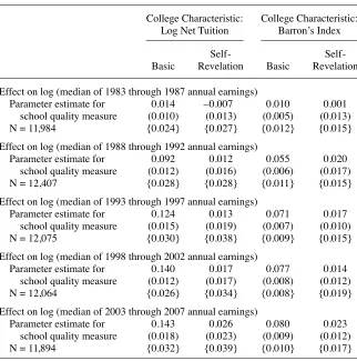
We estimated these same regressions for two other college characteristics, the Bar-ron’s index and the log of net tuition. The results are summarized in Table 6. In our basic model, the estimated impact of these school characteristics increased over the course of the student’s career, with the coeffi cient on log tuition reaching a high of 0.14 and the Barron’s index reaching 0.08 in the last fi ve- year interval (last set of rows, Table 6).17 However, in the self- revelation model, the estimates fall substantially and are statistically insignifi cant at the 0.10 level.18
16. This lower return to college selectivity for women is consistent with other literature. Results from Hoeks-tra (2009), Black and Smith (2004), and Long (2008) all suggest that the effect of college selectivity on earn-ings is lower for women than for men. Also, although the coeffi cients for school SAT in the self- revelation model were negative and signifi cant for women in some years, the pattern of results across all of the models we estimated (which included, for example, different measures of college quality and different minimum wage thresholds) did not suggest that the return for women was signifi cantly less than zero. For example, the coeffi cients for the Barron’s index for women was 0.051 (0.011) in the basic model and 0.010 (0.022) in the self- revelation model in 1993 to 1997; similarly, in 1998 through 1992, the coeffi cient was 0.050 (0.008) in the basic model and –0.004 (0.027) in the self- revelation model.
17. In exploratory analyses with the C&B data, we combined the measures of college quality using one of the empirical strategies suggested by Black and Smith (2006); specifi cally, we fi rst predicted school SAT score from net tuition and the Barron’s index and then estimated the effect of predicted school SAT score on earnings. The coeffi cient on predicted school SAT score was high: 0.126 with a standard error of 0.011 (compared to an estimate of 0.074 with a standard error of 0.016 if we use actual SAT score). However, the estimates fell substantially in our selection- adjusted models to an estimate of 0.044 (with a standard error of 0.012) when we control for the quality of schools the student applied to and to –0.028 with a standard error of 0.030 if we control for the quality of the colleges that accepted the students.
Dale and Krueger Table 5
Effect of School SAT Score / 100 on Earnings, 1976 Cohort
Men Women Men and Women Pooled
Basic
Self-
Revelation Basic
Self-
Revelation Basic
Self- Revelation
Effect on log (median of 1983 through 1987 earnings)
Parameter estimate for school SAT / 100 0.020 0.005 –0.010 –0.039 0.006 –0.015 (0.008) (0.011) (0.007) (0.012) (0.005) (0.008) {0.015} {0.019} {0.012} {0.016} {0.012} {0.015}
N 6,294 6,294 5,690 5,690 11,984 11,984
Effect on log (median of 1988 earnings through 1992 earnings)
Parameter estimate for school SAT / 100 0.063 0.009 0.028 –0.037 0.048 –0.011 (0.009) (0.013) (0.009) (0.015) (0.006) (0.010) {0.014} {0.018} {0.015} {0.020} {0.013} {0.013}
N 6,911 6,911 6,294 6,294 12,407 12,407
Effect on log (median of 1993 earnings through 1997 earnings)
Parameter estimate for school SAT / 100 0.091 0.001 0.031 –0.062 0.064 –0.021 (0.010) (0.016) (0.011) (0.018) (0.007) (0.012) {0.013} {0.015} {0.012} {0.016} {0.013} {0.014}
N 6,896 6,896 5,179 5,179 12,075 12,075
The Journal of Human Resources
Table 5 (continued)
Men Women Men and Women Pooled
Basic
Self-
Revelation Basic
Self-
Revelation Basic
Self- Revelation
Effect on log (median of 1998 earnings through 2002 earnings)
Parameter estimate for school SAT / 100 0.097 0.012 0.035 –0.076 0.070 –0.024 (0.012) (0.018) (0.012) (0.020) (0.008) (0.013) {0.015} {0.023} {0.013} {0.016} {0.013} {0.020}
N 6,869 6,869 5,195 5,195 12,064 12,064
Effect on log (median of 2003 earnings through 2007 earnings)
Parameter estimate for school SAT / 100 0.094 0.017 0.051 –0.040 0.074 –0.007 (0.013) (0.020) (0.012) (0.021) (0.009) (0.014) {0.016} {0.028} {0.017} {0.022} {0.015} {0.018}
N 6,650 6,650 5,244 5,244 11,894 11,894
Source: C&B Survey and Detailed Earnings Records from the Social Security Administration.
Dale and Krueger 343
Table 6
Effect of College Characteristics on Earnings, 1976 Cohort of Men and Women
College Characteristic: Log Net Tuition
College Characteristic: Barron’s Index
Basic
Self-
Revelation Basic
Self- Revelation
Effect on log (median of 1983 through 1987 annual earnings)
Parameter estimate for 0.014 –0.007 0.010 0.001
school quality measure (0.010) (0.013) (0.005) (0.013)
N = 11,984 {0.024} {0.027} {0.012} {0.015}
Effect on log (median of 1988 through 1992 annual earnings)
Parameter estimate for 0.092 0.012 0.055 0.020
school quality measure (0.012) (0.016) (0.006) (0.017)
N = 12,407 {0.028} {0.028} {0.011} {0.015}
Effect on log (median of 1993 through 1997 annual earnings)
Parameter estimate for 0.124 0.013 0.071 0.017
school quality measure (0.015) (0.019) (0.007) (0.010)
N = 12,075 {0.030} {0.038} {0.009} {0.015}
Effect on log (median of 1998 through 2002 annual earnings)
Parameter estimate for 0.140 0.017 0.077 0.014
school quality measure (0.012) (0.017) (0.008) (0.012)
N = 12,064 {0.026} {0.034} {0.008} {0.019}
Effect on log (median of 2003 through 2007 annual earnings)
Parameter estimate for 0.143 0.026 0.080 0.023
school quality measure (0.018) (0.023) (0.009) (0.012)
N = 11,894 {0.032} {0.039} {0.010} {0.017}
Source: C&B Survey and Detailed Earnings Records from the Social Security Administration.
These results are partly a contrast to Dale and Krueger (2002), in that the earlier analysis of self- reported earnings data showed a statistically signifi cant relationship between earnings and the log of net tuition in the self- revelation model because the coeffi cient on net tuition was 0.058 (0.018). To attempt to reconcile these results with Dale and Krueger (2002), we reestimated the effect of net tuition on self- reported earnings for full- time workers from the C&B survey in 1995 using the subset of students from the schools participating in this study and found that the coeffi cient (adjusted for clustering) on the log of net tuition from the self- revelation model was somewhat smaller, 0.041 (0.038), and not statistically signifi cant. When we estimated the same regression for the same sample but used SSA’s administrative earnings data in 1995 (instead of self- reported earnings data from the C&B survey), the coeffi cient (standard error) on net tuition was even smaller: 0.033 (0.046). Moreover, over the full study period (1983 to 2007) the coeffi cient on net tuition was generally between 0 and 0.02 (and never greater than 0.033) in the self- revelation model based on earnings drawn from SSA administrative data as the outcome measure. Thus, the effect of net tuition based on the single year of self- reported earnings reported in Dale and Krueger (2002) appears to been atypically high relative to the series of estimates we were able to generate using SSA’s administrative data, though the large standard errors make it diffi cult to draw inferences.
C. Estimated effects of college characteristics for the 1989 cohort
Unlike the 1976 cohort, where we have data for most of the student’s career, we only have a limited number of postcollege years for the 1989 cohort. As shown for the 1976 cohort, there is no return to college characteristics in the early part of a student’s ca-reer, possibly because many graduates from highly selective colleges attend graduate school and thus forego work experience early in their careers. Therefore, for the 1989 cohort, we focus on the most recent year with earnings data available, 2007, when the students were on average 35 years old. Although the 1989 cohort is too young for us to assess changes in the return to school selectivity over the student’s career, results for this cohort do allow us to assess whether estimates for the return to school selectivity are similar across cohorts at one point in the life cycle.
In 2007, the coeffi cient for school SAT score / 100 was 0.056 with a standard error of 0.014 (or 0.031 if we adjust for clustering among students who attended the same schools) in the basic model (Table 7). Consistent with the results for the 1976 cohort, the coeffi cient was indistinguishable from zero (–0.008 with a standard error of 0.019) in the self- revelation model. The results for each gender are also similar to those of the 1976 cohort: the coeffi cient for women (0.032) was lower than the coeffi cient for men (0.067) in the basic model; in the self- revelation model, estimates for both men and women are indistinguishable from zero (not shown). The results for the Barron’s index were consistent with the results for school SAT score. Specifi cally, the return to the Barron’s index was nearly 7 percent in the basic model but was close to zero in the self- revelation model. For net tuition, our estimates from both models were negative and had large standard errors.19
Dale and Krueger Table 7
Effect of College Characteristics on 2007 Earnings, 1989 Cohort of Men and Women
College Characteristic
School SAT Score / 100 Log Net Tuition Barron’s Index
Basic
Self-
Revelation Basic
Self-
Revelation Basic
Self- Revelation
Parameter estimate for 0.056 –0.008 –0.011 –0.108 0.069 –0.002 effect of quality measure (0.014) (0.019) (0.025) (0.028) (0.017) (0.022) on log 2007 earnings {0.031} {0.034} {0.062} {0.070} {0.038} {0.042}
Sample size 6,479 6,479 6,479
Source: C&B data and Detailed Earnings Records from the Social Security Administration.
D. Estimated effect of college characteristics for racial and ethnic minorities
Because some past studies have found that the return to college selectivity varies by race (Behrman, Rosenzweig, and Taubman 1996; Long 2009; Loury and Garman 1995), we also examined results separately for racial and ethnic minorities. To in-crease the sample size, we pooled blacks and Hispanics together because both groups often receive preferential treatment in the college admissions process (Bowen and Bok 1998). For the 1976 cohort, the effect of each college characteristic increased over the course of the student’s career, and the magnitude of the coeffi cients did not fall substantially in the self- revelation model. However, the estimate in the self- revelation model was not statistically signifi cant at the 0.10 level because of large standard errors (not shown, but available upon request).
For the black and Hispanic sample within the 1989 cohort, parameter estimates for each college characteristic ranged from 6.3 for the Barron’s index to 17.3 percent for the log of net tuition (Table 8). These estimates remained large in the self- revelation model, ranging from 4.9 for the Barron’s index to 13.8 for the log of net tuition. Although the standard errors are also large, some of the estimates are signifi cantly greater than zero. For example, the coeffi cient on school SAT score / 100 was 0.076 with a standard error of 0.032 (or 0.042 after accounting for clustering of students within schools).
Because the historically black colleges and universities in this sample had lower average SAT scores (and lower Barron’s indices and net tuition) than did the rest of the institutions in the C&B database, we investigated whether the large effect of school selectivity in 1989 for minority students was due to the greater range in school selec-tivity observed for minority students.20 Specifi cally, we reestimated the regressions but excluded the HBCUs from the sample. For the 1989 cohort, the estimates for minority students were even larger and were statistically signifi cant (at the 0.05 level) for the Barron’s index and for school SAT score when we excluded the HBCUs (not shown).21
E. Estimated effect of school average SAT score by parental education
Finally, we explored whether the effect of college selectivity varied by average years of parental education.22 The interaction term for school average SAT and years of parental education was negative for both cohorts, implying a higher payoff to attend-ing a more selective school for students from more disadvantaged family backgrounds (Table 9). For example, in the self- revelation model for the 1989 cohort, our results suggest that attending a college with a 200- point higher average SAT score would lead variable, the coeffi cient (and standard error) on net tuition in the basic model was 0.061 (0.038) and –0.035 (0.041) in the self- revelation model. (In contrast, adding a liberal arts dummy did not qualitatively change our fi ndings for the return to college average SAT score.)
20. See Fryer and Greenstone (2010) for estimates of the effect of HBCUs on earnings.
21. For the black and Hispanic subgroup of the 1976 cohort, estimates of the effects of school characteristics on earnings were smaller in magnitude when we excluded HBCUs compared to when we included HBCUs. However, each of these estimates had large standard errors and were statistically insignifi cant.
Dale and Krueger Table 8
Effect of School Characteristics on 2007 Earnings (Black and Hispanic Students Only, 1989 Cohort)
School SAT Score / 100 Log Net Tuition Barron’s Index
Dependent Variable Basic
Self-
Revelation Basic
Self-
Revelation Basic
Self- Revelation
All black and Hispanic students
Parameter estimate for 0.067 0.076 0.173 0.138 0.063 0.049 effect of quality measure (0.019) (0.032) (0.056) (0.071) (0.022) (0.036) on log 2007 earnings {0.028} {0.042} {0.076} {0.092} {0.033} {0.046}
Sample size 1,508 1,508 1,508
Source: C&B Survey and Social Security Administration’s Detailed Earnings Records.
The Journal of Human Resources
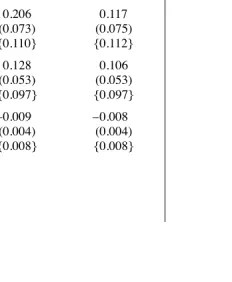
Table 9
Parameter Estimates from Earnings Regressions, Allowing the Effect of Average School SAT to Vary by Parental Education
Parameter Estimates
1976 Cohort 1989 Cohort
Variable Basic
Self-
Revelation Basic
Self- Revelation
School SAT score / 100 0.126 0.041 0.206 0.117
(0.035) (0.036) (0.073) (0.075) {0.058} {0.055} {0.110} {0.112}
Average years of parental education 0.066 0.063 0.128 0.106 (0.027) (0.027) (0.053) (0.053) {0.041} {0.038} {0.097} {0.097}
Dale and Krueger
Effect of a 200- point increase in school SAT score if Average years of parental education = 12 (equivalent to
high school graduate)
0.148 –0.025 0.193 0.052
Average years of parental education = 16 (approximately equivalent to college graduate)
0.113 –0.060 0.120 –0.009
Average years of parental education = 19 (approximately equivalent to graduate degree)
0.087 –0.087 0.065 –0.055
Sample size (unweighted) 12,053 12,053 6,466 6,466
Source: C&B data and Detailed Earnings Records from the Social Security Administration.
to 5.2 percent higher earnings in 2007 for those with average parental education of 12 years (equivalent to graduating from high school). However, for those whose par-ents averaged 16 years of education (approximately equivalent to college graduates), there was virtually no return to attending a more selective college. Similar to Dale and Krueger (2002), we also found a negative interaction between predicted parental income and school average SAT score though the interaction term was generally not statistically signifi cant.
VI. Conclusion
Consistent with the past literature, we fi nd a positive and signifi cant effect of college selectivity during a student’s prime working years in regression mod-els that do not adjust for unobserved student quality for cohorts that entered college in 1976 and 1989 using administrative earnings data from the SSA’s Detailed Earnings Records. Based on these same regression specifi cations, we also fi nd that the effect of college selectivity increases over the course of a student’s career. However, after we partially adjust for unobserved student characteristics (by controlling for the average SAT score of the colleges students applied to) in our “self- revelation” model, the ef-fect of college selectivity falls dramatically. For the 1976 cohort, the efef-fect of school SAT score for the full sample is indistinguishable from zero in the self- revelation model. Similarly, the effects of other college characteristics (the Barron’s index and net tuition) are substantial in regressions that control for commonly observed student characteristics but small and not statistically distinguishable from zero in the self- revelation model.
There were noteworthy exceptions for subgroups. First, for the 1989 cohort, the estimates indicate the effect of attending a school with a higher average SAT score is positive for black and Hispanic students, even in the selection- adjusted model. Second, our results suggest that students from disadvantaged family backgrounds (in terms of educational attainment) experience a greater benefi t from attending a college with a higher average SAT score than do those from more advantaged family back-grounds. For example, for the 1989 cohort, our estimates from the selection- adjusted model imply that the effect of attending a college with a higher average SAT score is positive for students whose parents had an average of fewer than 16 years of school-ing; however, the effect of attending a more selective college was zero (or even nega-tive) for students whose parents averaged 16 or more years of education. One possible explanation for this pattern is that although most students who apply to selective col-leges may be able to rely on their families and friends to provide job- networking op-portunities, networking opportunities that become available from attending a selective college may be particularly valuable for black and Hispanic students and for students from less educated families.
Dale and Krueger 351
6 percent higher earnings (in 1995 and 2007, respectively) according our basic model; for both cohorts, this effect was close to zero in our selection- adjusted model.
Our fi ndings have several caveats. First, the analysis does not pertain to a nationally representative sample of schools because the sample is derived from 27 colleges and universities in the C&B data set, the majority of which are very selective. However, estimates of the effects of school selectivity based on the C&B data set were similar to—indeed, slightly higher than—those based on a nationally representative data set, the NLS- 72. (See Dale and Krueger 2002.) In addition, Dale and Krueger (2002) found an insignifi cant payoff to attending more selective schools when they used the NLS to estimate the self- revelation model. Thus, although the results reported in this paper are based on students that mainly attended moderately selective or very selective schools, it is not clear that we would have obtained different results from a nationally representative data set.
Second, the estimates from the selection- adjusted models are imprecise, especially for the 1989 cohort. Thus, even though the point estimates for the effect of a college characteristic are close to zero, the upper bound of the 95 percent confi dence intervals for these estimates are sometimes sizeable. Also, our estimates are based on a single proxy for school quality and therefore may be understated relative to estimates are based on multiple proxies for school quality as explained by Black and Smith (2006). Nonetheless, our results do suggest that estimates that do not adjust for unobserved student characteristics are biased upward.
Finally, it is possible that our estimates are affected by students sorting into the colleges they attended based on their unobserved earnings potential. About 35 percent of the students in each cohort in our sample did not attend the most selective school to which they were admitted.23 Our analysis indicates that students (especially those from the 1976 cohort) who were more likely to attend the most selective school to which they were admitted tended to have observable characteristics that are associated with higher earnings potential. If unobserved characteristics bear a similar relation-ship to college choice, then our already small estimates of the payoff from attend-ing a selective college would be biased upward. It is also possible that the benefi t in terms of future earnings from attending a selective college varies across students and that students sort into college based on their perceived costs and benefi ts. Very selective colleges may attract not only students with very high family incomes (who can afford tuition) but also those with low family incomes (who receive fi nancial aid). Conversely, students who expect a lucrative career because they intend to earn an MBA after college (for example) may sort into less selective undergraduate colleges. If students sort on the basis of their idiosyncratic return from attending a selective college, then Equation 1 cannot be given a causal interpretation. However, if this is the case, then the typical student does not unambiguously benefi t from attending the most selective college to which he or she was admitted. Rather, students need to think carefully about the fi t between their abilities and interests, the attributes of the school they attend, and their career aspirations.
The Journal of Human Resources
Appendix
Table A1
Characteristics of College and Beyond Schools Included in Study
1976 Cohort 1989 Cohort
Institution
SAT Percentile Relative to All 4- Year Institutions
(1992)
1978 Average SAT Score
1976 Net Tuition ($)
1978 Barron’s
Index
1992 Average SAT Score
1990 Net Tuition ($)
1992 Barron’s
Index
Barnard College 97 1210 3,530 4
Bryn Mawr College 99 1370 3,171 5 1285 11,905 5
Columbia University 99 1330 3,591 5
Duke University 99 1226 3,052 4 1285 12,219 5
Emory University 96 1150 3,237 3
Georgetown University 97 1225 3,304 4 1235 12,141 5
Hamilton College 95 1246 3,529 4
Miami University (Ohio) 95 1073 1,304 2 1154 3,018 4
Morehouse 76 830 1,549 2 998 5,601 3
Northwestern University 98 1240 3,676 4
Oberlin College 97 1227 3,441 4 1216 15,738 5
Pennsylvania State University 90 1038 1,062 2 1083 5,426 3
Dale and Krueger
Smith College 95 1210 3,539 5
Stanford University 99 1270 3,658 5 1351 11,127 5
Swarthmore College 99 1340 3,122 5
Tufts University 98 1200 3,853 4
Tulane University 95 1080 3,269 3
University of Michigan 95 1110 1,517 3 1164 6,595 4
University of Notre Dame 98 1200 3,216 4
Vanderbilt University 96 1162 3,155 3 1177 11,030 4
Washington University 97 1180 3,245 3 1201 11,267 5
Wellesley College 98 1220 3,312 5 1240 11,358 5
Wesleyan University 98 1260 3,368 5 1284 12,688 5
Williams College 99 1255 3,541 5 1329 13,249 5
Xavier 68 710 1,326 4 966 5,391 2
Yale University 99 1360 3,744 5 1379 13,366 5
Source: American Council on Education (1973, 1983, 1992) (for net tuition); Barron’s (1978) and College Division of Barron’s Education Series (1992) (for Barron’s index in 1978 and 1992 and school SAT scores in 1992); the Higher Education Research Institute (for school SAT scores in 1978).
Table A2
Relationship Between Student Characteristics and Average SAT Score / 100 of College Attended
Correlation with College Average SAT Score
Parameter Estimate for Effect of Student Characteristic on College
Average SAT Score of School Attended 1976 Cohort 1989 Cohort 1976 Cohort 1989 Cohort
Predicted parental 0.182 0.278 –0.020 0.049
income < 0.001 < 0.001 (0.013) (0.016)
Student SAT score / 100 0.511 0.579 0.060 0.049
< 0.001 < 0.001 (0.060) (0.004)
High school grade 0.265 0.200 0.114 –0.052
point average < 0.001 < 0.001 (0.014) (0.024)
Female 0.016 0.023 0.084 0.067
0.035 0.033 (0.009) (0.001)
Black –0.184 –0.232 –0.066 –0.086
< 0.001 < 0.001 (0.019) (0.022)
Hispanic 0.062 0.084 0.305 0.192
< 0.001 < 0.001 (0.043) (0.033)
Asian 0.090 0.160 0.113 0.036
< 0.001 < 0.001 (0.030) (0.020)
Other race –0.041 0.029 –0.132 0.260
< 0.001 0.006 (.022) (0.076)
Source: C&B Survey.
355 Table A3
Full Set of Parameter Estimates for Selected Log of Earnings Regressions
1976 Cohort 1989 Cohort
School SAT score / 100 0.061 –0.023 0.056 –0.008
(0.013) (0.014) (0.031) (0.034)
Student SAT score / 100 0.022 0.014 0.047 0.033
(0.005) (0.005) (0.008) (0.008)
Student SAT missing –0.141 –0.122 –0.262 –0.217
(0.030) (0.030) (0.160) (0.160)
High school GPA 0.218 0.216 0.194 0.188
(0.021) (0.021) (0.042) (0.042)
High school GPA missing 0.015 0.013 0.094 0.092
(0.014) (0.014) (0.021) (0.021)
Predicted parental income 0.161 0.140 0.137 0.117
(0.019) (0.017) (0.029) (0.029)
Athlete 0.124 0.123 0.135 0.092
(0.025) (0.037) (0.037) (0.020)
Average SAT score / 100 of 0.100 0.099
schools applied to (0.012) (0.014)
One additional application 0.062 0.029
R- squared 0.147 0.153 0.122 0.126
Sample size (unweighted) 12,075 6,479
Source: C&B Survey and Detailed Earnings Records from the Social Security Administration.