BENDING THE DOMING EFFECT IN STRUCTURE FROM MOTION
RECONSTRUCTIONS THROUGH BUNDLE ADJUSTMENT
L. Magria, R. Toldob,∗
a
Dip. Informatica - Universit`a di Verona - Strada Le Grazie 15, Verona, Italy - [email protected] b
3Dflow SRL, c/o Computer Science Park - Strada Le Grazie 15, Verona, Italy
KEY WORDS:Bundle Adjustment, Doming effect, Ground detection
ABSTRACT:
Structure from Motion techniques provides low-cost and flexible methods that can be adopted in arial surveying to collect topographic data with accurate results. Nevertheless, the so-called “doming effect”, due to unfortunate acquisition conditions or unreliable modeling of radial distortion, has been recognized as a critical issue that disrupts the quality of the attained 3D reconstruction. In this paper we propose a novel method, that works effectively in the presence of a nearly flat soil, to tacklea posteriorithe doming effect: an automatic ground detection method is used to capture the doming deformation flawing the reconstruction, which in turn is wrapped to the correct geometry by iteratively enforcing a planarity constraint through a Bundle Adjustment framework. Experiments on real word datasets demonstrate promising results.
1. THE DOMING EFFECT
In recent years Structure from Motion techniques have enjoyed increasing popularity in the context of aerial surveying – where have been used in several applicative scenarios, ranging from earth science to heritage documentation – thanks to their ability to provide detailed imagery and accurate 3D models, by exploit-ing a flexible and low cost equipment, such as consumer-grade cameras.
Unfortunately, despite this appealing feature, Structure from Mo-tion methods may be affected with two major problems. First, the incremental nature of Structure from Motion, which itera-tively builds up a 3D model by alternating between camera pose and scene points estimates, suffers fromdrifting(Cornelis et al., 2004): i.e. the propagation of errors, due to noisy measurements, accumulated through the reconstruction process. As a remedy, Bundle Adjustment is routinely adopted to jointly refine the 3D structure of the scene together with the viewing parameters of the acquisition setup. Second, inaccuracies in modeling the ra-dial distortion of camera lens (Fryer and Mitchell, 1987) (which may commonly occur in many self-calibration procedure) are re-flected in the so called “doming” effect: a broad-scale systematic deformation of the reconstructed surface which often appears as a rounded-vault-distortion of flat surface – as recognized exper-imentally for example in (Rosnell and Honkavaara, 2012, Javer-nick et al., 2014, Ou´edraogo et al., 2014). Interestingly, from a theoretical point of view, this phenomenon is related to critical loci arisen in the context of radial distortion self calibration (Wu, 2014). In practice, (James and Robson, 2014, Smith and Ver-icat, 2015) observe that the doming effect is particular evident for UAV systems that take images from near-parallel directions, causing systematic errors in the associated DEM. The rundown of these studies is that the doming effect may be alleviated with a careful design of a distributed network of ground points or by taking slightly off-vertical convergent imagery. However, even if these solutions succeed in reducing the amount of deformation, they do not remove its systematic nature and are limited only to laborious controlled setting.
∗Corresponding author
Contributions In this work we present a novel solution to deal with the doming effect that mitigates the need of these precau-tions during the acquisition phase by correcting the deformation during the reconstruction step. In particular, under the assump-tion of a known geometry of the terrain,e.g.an approximate flat soil, we show how it is possible to compensate the doming defor-mation by enforcing a planarity constraint over a set of automati-cally selected points on the ground within the Bundle Adjustment framework. The main idea is to extract the relevant information to guide the Bundle Adjustment optimization by leveraging on a simple-to-implement robust model fitting technique that auto-matically assess and quantify the amount of doming deforma-tion. In this way, we are able to allow accurate reconstructions in a wider array of circumstances. For example, this method will increase the quality of the attained 3D model when the adopted cameras manifest some unavoidable radial distortion or have been modeled in a defective way. In addition, the proposed approach can also deal with challenging acquisition scenarios,e.g. when oblique images are not available, or when it is difficult to define a careful designed net of control points.
This manuscript is structured as follows, a first overview of the method in Section 2 is followed by the description of the two main steps of the suggested solutions, namely ground detection in Section 3 and constrained Bundle Adjustment in Section 4. Sample results attained on real datasets are provided in Section 5.
2. OVERVIEW
Our method in a nutshell can be presented as follows. Starting from a tentative 3D reconstruction of the scene, before Bundle Adjustment is carried on, a robust model fitting technique is used to detect the ground, which is geometrically approximate either as a plane or as a second order surface, depending on the amount of the deformation. In this work we employ elliptic paraboloids to describe the domed deformation of the terrain, and we derive anad hocconstrained-type least square fitting method.
Ground detection
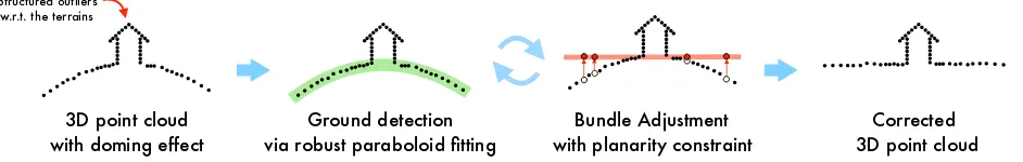
Figure 1. An overview of the main steps of the proposed method. At first the domed terrain is extracted from the point cloud via a robust paraboloid fitting technique. Hence points on the ground are selected and used to enforce a planarity constraint within an iterative Bundle Adjustment framework.
therefore, we exploits a robust framework, based on LMedS, com-bined with an outlier diagnostic criterion, to extract from the 3D point cloud the ground, either in the form of a plane or a paraboloid. The structure that has the least median of squared residuals is used to approximate the soil geometry. Residuals be-tween points and the attained structures are computed, hence, a Forward Search procedure, based on the scrutiny of this residual distribution, is used to prune outliers and identify points laying on the ground. If the recovered structure happens to be a plane, the doming effect can be considered negligible, otherwise some of the inliers of the estimated paraboloid are used as control points and constrained to be coplanar in the subsequent Bundle Adjust-ment optimization. The procedure is iteratively repeated until the detected ground happen to be correctly flattened to the soil plane. An high-level illustration of this strategy is pictorially sketched in Figure 1.
3. GROUND DETECTION
We split up the problem of automatically extract the terrain from a 3D reconstruction of a scene in two sub-problems which are re-spectively addressed in the following two sections.
The first issue is the geometric description of the deformed ter-rain. While flat soil can be straightforwardly represented by a plane, fitting a second order surface to a domed terrain is a more challenging task, because, without further restraints, the estima-tion of a generic quadric surface may yield, in presence of noise and occlusions, to different kinds of quadrics and may also get stuck in degenerate cases that do not capture adequately the dom-ing effect. For these reasons, in the next section, we conceive a simple and direct specific-paraboloid least-square fitting method that avoids these difficulties.
The second problem to deal with is robustness, which is discussed in Section 3.2 where LMedS and Forward Search are presented.
3.1 Specific paraboloid fitting
Elliptic paraboloids are manageable parametric models that well represent the doming deformation. They are special instances of quadric surfaces. A general quadric surface can be represented as the vanishing locus of a second order polynomial of the form
F(Q,X) =X⊤QX= 0 (1)
whereQis a4×4real symmetric matrix andX= [x, y, z,1]⊤ denotes a point in the euclidean space in homogeneous coordi-nates.F(Q,X)represents the algebraic distance of a pointXto the quadricQ. Given a sparse cloud ofnpointsX ={Xi}ni=1, the general problem of fitting a quadric may be tackled via a least square approach by minimizing the sum of squared algebraic dis-tances
In order to avoid the trivial solutionQ≡0, the entries ofQmay be constrained to satisfy a relation of some kind. We recall that two matricesQ,Q′ that differ for a multiplicative factor, repre-sent the same quadric, therefore we have the freedom to arbitrar-ily scale the entries ofQ.
This feature can be favorably exploited to derive a quadratic con-strain to force the quadric to be an elliptic paraboloid. This idea was firstly suggested by (Fitzgibbon et al., 1999) for the problem of fitting an ellipse in the plane. Here we revisit and generalize to our paraboloid fitting scenario this approach. The main advan-tages are: (i) ensure some desirable features∗that well describe the geometry of the soil to the fitted surface – namely, the sur-face is composed by a single connected component, the nature of the points iselliptical(i.e. a point of the surface is elliptic if the surface in its neighborhood is on the same side of the tangent plane) (ii) avoid degenerate cases in the presence of noise and occlusions.
We recall thatQrepresents an elliptic paraboloid if and only if the following two conditions on the so calledorthogonal invariants hold
We confine our discussion to paraboloids having the principal axis vertically aligned, as we assume that the reference system has the z-axis pointing towards the zenith. In this case Equa-tion (1) can be further simplify as
a1x2+a2xy+a3y2+a4x+a5y+a6z+a7= 0, (4)
and the corresponding quadric matrix turns out to be
Q=
in this way the conditionI3 = 0is always satisfied. As regards
the constraintI4 <0, with some calculations, it can be reduced
to
a1a3−a 2 2
4 >0. (6)
Rather than working with this inequality, which in general is dif-ficult to deal with, we take advantage of the freedom to arbitrarily scale the entries ofQ: we simply integrate the scaling factor into
Equation (6) by enforcing the equality
By wrapping up the quadric parameters in vectorial form asa= [a1, a2, a3, a4, a5, a6, a7]⊤, we can rephrase more compactly this
condition as a quadratic constrainta⊤Ca= 1of the form
a⊤
In summary, starting from the problem in Equation (2), we end up with the following constrained fitting problem
minkDak2constrained toa⊤Ca= 1 (9)
This problem can be efficiently solved, as explained in (Fitzgib-bon et al., 1999), by retaining as a solution the eigenvectorˆathat corresponds to the single negative generalized eigenvalue of the associated generalized eigenproblem
(
D⊤Da=λCa
a⊤Ca= 1. (11)
3.2 Robust estimation technique
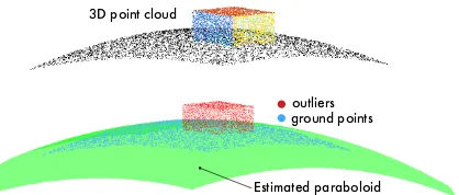
The reconstructed scene may include many structured points that do not lie on the soil and that act as outliers during the terrain extraction phase, as illustrated at the top of Figure 2. In presence of such outlying measurements, our specific-paraboloid fitting method, being a simple constrained least squares technique, will break down. Therefore, in order to compensate for its fragility, we integrate the ground detection step in a robust estimation frame-work based on the Least Median of Squares (LMedS) coupled with Forward Search to prune outliers at the end. An example of the results yielded by this robust approach on an instance of synthetic data is depicted at the bottom of Figure 2.
Least Median of Squares LMedS is a robust regression tech-nique that achieves the maximum theoretical breakdown point of 0.5,i.e., it can tolerate up to 50% percent of outliers in the data without being affected. At high level, if we denote byri,athe Euclidean distance between thei-th pointxiand a model deter-mined bya, the LMedS estimate is given by:
ˆ
a= arg min
a median
xi∈Xri,2a, (12)
that is, the estimate must yield the smallest value for the median of squared residuals computed for the entire data set.
The parametersaare obtained via random sampling: a number of subsetsS ⊂X composed by the minimum number of points
3D point cloud
Estimated paraboloid outliers ground points
Figure 2. Ground detection with robust paraboloid fitting. A toy example with synthetic dataTOP: the input data are given by the points on a paraboloid and points on a box lying on top of it (colored for visualization purpose). Gaussian noise is added on point coordinatesBOTTOM: the paraboloid estimated via LMedS is displayed in green. Forward Search is used to dichotomize between inliers in light blue and outliers in red.
necessary to instantiate a model (e.g. 3points for instantiate a plane or7to fit a paraboloid) are randomly selected from the data, and a parameter vectoraSis fitted to the points in each sub-set. Hence, eachaSis tested by calculating the squared residual distancer2
i,aS of each of then−kpoints inX−Sand the me-dian of the residuals is computed. TheaScorresponding to the smallest median is chosen as the estimateaˆ. Ifnis the number of points in the initial set of data, there are nk
different subsets ofkpoints that should be considered. In order to speed up the process, the number of subsets to test can be reduced to
M = log(1−p)
log(1−(1−ǫ)k), (13)
wherepis the probability of calculating the correct estimate and ǫis the percentage of outliers.
In our scenario we found beneficial to adopt a simple bucketing technique to encourage the sampling of well separated points, in order to reduce the standard error on the estimated parameter by leveraging on data that are more spread out.
It is known that, when in addition to outliers, Gaussian noise is present, the relative statistical efficiency of LMedS is low.
Therefore, to compensate for this deficiency, it is important to re-fine the fit on a outliers-free set of data. To this end, a common practice is to adopt scale estimation strategies to dichotomize be-tween noisy inliers and gross outliers. Along this line, common solutions consist in univariate single-step outlier detection pro-cedures that reject those points whose residuals are greater than a certain threshold. This threshold can be fixed in advance or computed adaptively from the data, for example using the me-dian absolute deviation (MAD). Other solutions involve the use of sequential procedures that monitor the distribution of residu-als either byinward testing, that performs successive elimination of points with high residual, or byoutward testing, that adds se-quentially points to the inlier set until a certain criterion is met.
estimat
ed inlier t
hr
eshold
residual distribution
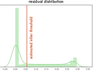
Figure 3. The distribution of the residuals computed w.r.t. the paraboloid estimated from LMedS on the toy example of Figure 2, together with the inlier threshold (red line) obtained via For-ward Search.
the parameters of the modelasand thes+ 1residualrs+1,as is checked to detect the point when the iteration starts including outliers.
Among the several monitoring heuristics proposed in literature, we consider here one of the simplest, that dates back to (Hadi and Simonoff, 1993). The forward search stops when:
rs2+1,as≥(t(1−α/2(s+1),s−k)σs)2 (14)
wheret(1−α/2(s+1),s−k) is the1−α/2(s+ 1)quantile of the
t-distribution withs−kdegrees of freedom, andσsis the stan-dard deviation of the leastsresiduals (the residual divided byσs is also called “studentized” residual). The main idea is to recog-nized the first point whose residual does not follow the gaussian distribution of the inlier to the model.
Thei-th iteration of the algorithm can be summarized as follows:
1. Estimate the parameters of the modelasusing thes=m+ i−1points in the clean subset;
2. Calculate the residualsrs+1,as of all thenpoints and ar-range them in ascending order;
3. Test the(s+ 1)thresidual:
Ifr2
s+1,as ≥(t(1−α/2(s+1),s−k)σs)2then declare all
the remainingn−sobservations as outliers and stop.
Otherwise incrementi(include the(s+ 1)thpoint in the inliers).
4. Ifm+i−1 =n, then stop, otherwise go to step 1.
We applied this procedure to the synthetic data presented in Fig-ure 2, and the results achieved are presented in FigFig-ure 3 where it can be appreciated the multi-modality of the residual distribution and how the estimated inlier threshold accurately dichotomized between inliers and structured outliers.
3.3 Model selection: flat or domed?
Our objective is to enforce a linear constraint on the domed ground, warping progressively into a plane the inliers points of the paraboloid retrieved by FS. Due to the iterative nature of this wrapping pro-cess, we need a mechanism to automatically assess when points
x
iπ
φ
(
t
)
Figure 4. The distance between a point and a paraboloid is re-duced to computing the distance between a point and a parabola in the plane.
on the paraboloid happen to be planar, or in other words, we need the ability to robustly detect both elliptic paraboloid and planes∗.
In general, this issue turns to be a tricky model selection problem that requires some kind of regularization based on suitable model complexity measures. Fortunately, for our purpose, we find that a simple extension of the LMedS framework, aimed at handling at the same time different kind of parametric models, works prof-itably. Specifically, we tailor LMedS to simultaneously instanti-ate tentative paraboloids and planes. In this way, by expressing residuals in the same geometric unit of measure, we are able to neatly compare the goodness of fit of sampled structures and to choose the proper geometric primitive. Please note that the adop-tion of our specific-paraboloid fitting method is crucial for the success of this approach: a generic quadric fitting method would produce a degenerate estimate in case of flat terrain leading to inconsistent results.
Mixed sampling strategy: The adjustments to LMedS apply exclusively to the sampling step. Paraboloids are instantiated from minimum sample set of7points whereas3D planes are ob-tained by sampling triplets of points. The geometric residual be-tween a pointxiand a plane, that is represented as a4parameter vectora, is easily computed as
ri,a=
|a⊤xi| p
a2
1+a22+a23
. (15)
When an elliptic paraboloid is considered, abecomes a7 pa-rameter vector, and the geometric residual ofxiis computed as follows (for reference see Figure 4):
1. the planeπpassing through the axis of the paraboloid and the pointxiis computed;
2. the parabola given by the intersection ofπand the paraboloid is determined and parametrized asφ(t);
3. the distance betweenxi and the parabola is calculated by finding the minimum of the squared normf(t) =kφ(t)−
xik2. This boils down to finding the roots of the third degree polynomial obtained by differentiatingf(t)with respect to t, that can be easily computed in closed form.
In order to avoid7-tuple of bad conditioned points, every time a minimum sample set is drawn, a planarity check is performed
and, if it is deemed as planar, a plane is instantiated and added to the pool of putative models.
LMedS, aside from the described mixed sampling strategy, is im-plemented in a straightforward way. The model selection simply boils down to select the structure, either plane or paraboloid, that obtains the least median of squares, which in turn is used to ap-proximate the ground and feed to Forward Search.
4. BUNDLE ADJUSTMENT WITH PLANAR CONSTRAINT
It is customary to adopt Bundle Adjustment (Triggs et al., 1999) to minimize the propagation of errors in Structure from Motion techniques in order to provide a jointly optimal estimate of 3D structure and viewing parameters. The terms “bundle” comes from the bundle of light rays that connects each camera center with the set of visible 3D points of the scene. This bundle of rays is adjusted via a proper optimization routine aimed at min-imizing the overall residual error,i.e., the distance between the re-projected 3D points and the corresponding measured image points, in formulas:
Pjis a3×4matrix encapsulating the interior and exterior orien-tations together with the radial distortion parameters of thej-th camera, Xirepresents thei-th points of the scene andxi,j its 2D homogeneous coordinates in thej-th image,d()indicates the Euclidean distance in the image plane. The coefficientswi,jare weights that indicates if a pointsXiis seen by a cameraPjand can also be used to mitigate the effect of gross measurements, down-weighting the influence of outliers (Zach, 2014). This non linear least weighted square problem can be efficiently resolved through several numerical implementations rooted in Gauss-Newton methods, that conveniently exploit the structure of the Jacobian associated to Equation (16), seee.g.(Agarwal et al., 2010, Kono-lige and Garage, 2010) for a review and a more detailed discus-sion.
We want to modify Equation (16) in order to guide Bundle Ad-justment to correct the camera parameters (including radial dis-tortion values) and the point locations towards a reconstruction in which the terrain is plane. Under the flat soil assumption, the positions of the inliers of the attained paraboloid are certainly in-accurate. Therefore, enforcing a planarity constraint on their lo-cations, is a useful cues that can be encompassed in the optimiza-tion process. With this idea in mind, we perform the following three steps:
1. At first we automatically pick a subset of ground points Xi∈U indexed byU ⊂ {1, . . . , n}among the inliers ob-tained via Forward Search.
2. Then, we linearly project the selected points onto a designed planeτ, obtaining new 3D positions – sayYiwithi∈ U.
3. At the end, we force the bundle of rays corresponding to the selected points to pass through the 3D positionsYi.
This means that Bundle Adjustment minimizes the re-projection error with respect to both the camera parameters and the 3D point positions for all the points, except the selectedXi i ∈ U for
LMedS
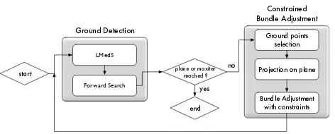
Figure 5. The flow chart of the proposed method
which the coordinates are kept fixed and equal to their planar pro-jectionsYi. Thus Equation (16) becomes
min
Selection of ground points The subsetUcorresponding to the selected ground points is obtained through a decimation heuristic based on a bucketing technique. Only points that are inliers to the attained quadric are taken into account. Hence, the space of the scene is divided in regular cells with predetermined width. For each nonempty cell the point that is nearest to the cell-center is selected and the corresponding index is put inU. In this way the selected points are well spread through the whole scene. An example of selected ground points in a real scene is presented in Figure 7.
Planar projection The planeτonto which points are projected is chosen to be the tangent plane to the estimated quadricQat a certain pointMon Q. The pointMcan be picked in several ways: the vertex of the paraboloid is a good candidate, alterna-tively it can be specified by the user. Given the coordinates ofM, the coefficients of the planeτ are simply found ast = M⊤Q. The projectionYionτ are computed via matrix multiplication Yi=HXi, where
H= (td⊤−(t⊤d)I)⊤, (18)
drepresents a direction of projection expressed in homogeneous
coordinates,e.g.v= [0,0,1,0]⊤, andIdenotes the4×4identity matrix.
Weights setting If thei-th points is visible from thej-th cam-era, the corresponding addend that appears in Equation (17) is robustly weighted by the coefficientswi,j. The weight is defined in terms of the re-projection error so to reduce the influence of contributions higher than a certain toleranceǫi:
wi,j(u) = (
1 ifu < ǫi
1/u otherwise. (19)
We set an higher toleranceǫifori∈ U because we want to in-crease the importance of the error relative to the selected ground points. In this way we are able to guide Bundle Adjustment towards a planar solutions. In practice, if we express the re-projection error in pixel, we fixǫi = 5 ifi ∈ U andǫi = 1 otherwise.
5. EXPERIMENTAL VALIDATION
Most Structure from Motion pipelines are either sequential –i.e.a two-view reconstruction is sequentially augmented by adding in a new image at each iteration – or hierarchical: input images are at first organized in a dendrogram based on a similarity measure and then, following the order defined by this structure, smaller re-constructions are progressively merged in a complete 3D model. In order to assess the results of our constrained Bundle Adjust-ment, we used a Structure from Motion technique belonging to the latter category. Specifically, we employed 3DF Zephyr Aerial which implements the hierarchical approach of SAMANTHA – a state-of-the-art Structure from Motion technique described in (Toldo et al., 2015). It is worth noting that, the camera parame-ters were kept fixed and jointly optimize by Bundle Adjustment for blocks of similar images grouped together by Samantha.
We took in consideration three datasets of sparse reconstructions obtained from aerial survey: villagecomposed by 6.323 points captured by 136 cameras,country lanecomposed by 18.059 points registered by 49 cameras, andbuildingsmade up of 18.655 points and 103 cameras. The first two acquisitions were taken from an higher distance with respect to the last one. In all the three cases the internal orientations of the cameras were flawed, in particu-lar, the radial distortion parameters were erroneously estimated. These unfavorable conditions resulted in a set of 3D points af-fected by the doming deformation, as can be seen in the first col-umn of Figure 6 where a top view of the three scenes together with the color-coded elevation of the points is presented. In vil-lage, where the vertex of the paraboloid of the doming effect is in the middle of the scene, it is particular easy to recognize the parabolic geometry of the terrain.
The point cloud obtained by our constrained Bundle Adjustment are collected in the right column of Figure 6, from which it can be appreciated that the doming effect has been considerably attenu-ated, confirming the usefulness of this approach. One can also observe that, at the same time, the overall details and the other structures of interest present in the scene have been preserved thanks to the careful choice of ground points to guide Bundle Ad-justment. For example, one can compare, the bottom-right corner of thebuildingdataset and recognized that the positions of the yellow points – which corresponding to a roof in the scene – have not been moved by Bundle Adjustment as they have been deemed as outliers with respect to the ground paraboloid.
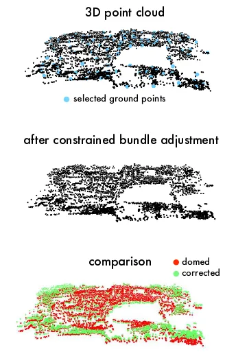
In Figure 7 a comparison between the input and the output point cloud on thevillagedatasets, qualitatively illustrate the transfor-mation induced by Bundle Adjustment which wraps the points towards a flat-soil geometry.
6. CONCLUSION AND FUTURE WORK
We have presented an effective method aimed at mitigating the doming effect. Our approach recover a correct reconstruction by properly integrating geometric clues in an iterative Bundle Ad-justment framework. Further investigations about the connec-tions between inaccuracies in the estimation of radial distortion parameters and the induced geometry of the deformed scene are in plan for future work. Moreover, a further advancement of this approach would be the introduction of a rematching phase of the keypoints at the end of the whole process. Also a careful study of the directiondthorugh which the planar projection is realized, would increase the accuracy of the attained reconstruction.
Figure 6. Top views of the doming effect on three datasets. The elevation values of the points is color-coded.
3D point cloud
selected ground points
after constrained bundle adjustment
comparison domed corrected
REFERENCES
Agarwal, S., Snavely, N., Seitz, S. and Szeliski, R., 2010. Bundle adjustment in the large.Computer Vision–ECCV 2010pp. 29–42.
Atkinson, A. and Riani, M., 2000.Robust Diagnostic Regression Analysis. Springer Series in Statistics, Springer.
Cornelis, K., Verbiest, F. and Van Gool, L., 2004. Drift detec-tion and removal for sequential structure from modetec-tion algorithms. IEEE Transactions on Pattern Analysis and Machine Intelligence 26(10), pp. 1249–1259.
Fitzgibbon, A., Pilu, M. and Fisher, R. B., 1999. Direct least square fitting of ellipses. IEEE Transactions on pattern analysis and machine intelligence21(5), pp. 476–480.
Fryer, J. and Mitchell, H., 1987. Radial distortion and close range stereophotogrammetry. Australian Journal of Geodesy, Photogrammetry and Surveying46(47), pp. 123–138.
Hadi, A. S. and Simonoff, J. S., 1993. Procedures for the iden-tification of multiple outliers in linear models. Journal of the American Statistical Association88(424), pp. pp. 1264–1272.
James, M. R. and Robson, S., 2014. Mitigating systematic error in topographic models derived from uav and ground-based im-age networks. Earth Surface Processes and Landforms39(10), pp. 1413–1420.
Javernick, L., Brasington, J. and Caruso, B., 2014. Modeling the topography of shallow braided rivers using structure-from-motion photogrammetry.Geomorphology213, pp. 166–182.
Konolige, K. and Garage, W., 2010. Sparse sparse bundle adjust-ment. In:BMVC, Vol. 10, pp. 102–1.
Ou´edraogo, M. M., Degr´e, A., Debouche, C. and Lisein, J., 2014. The evaluation of unmanned aerial system-based photogramme-try and terrestrial laser scanning to generate dems of agricultural watersheds.Geomorphology214, pp. 339–355.
Rosnell, T. and Honkavaara, E., 2012. Point cloud generation from aerial image data acquired by a quadrocopter type micro unmanned aerial vehicle and a digital still camera.Sensors12(1), pp. 453–480.
Smith, M. W. and Vericat, D., 2015. From experimental plots to experimental landscapes: topography, erosion and deposition in sub-humid badlands from structure-from-motion photogramme-try. Earth Surface Processes and Landforms40(12), pp. 1656– 1671.
Toldo, R., Gherardi, R., Farenzena, M. and Fusiello, A., 2015. Hierarchical structure-and-motion recovery from uncali-brated images. Computer Vision and Image Understanding140, pp. 127–143.
Triggs, B., McLauchlan, P. F., Hartley, R. I. and Fitzgibbon, A. W., 1999. Bundle adjustmenta modern synthesis. In: Interna-tional workshop on vision algorithms, Springer, pp. 298–372.
Wu, C., 2014. Critical configurations for radial distortion self-calibration. In: Proceedings of the IEEE Conference on Com-puter Vision and Pattern Recognition, pp. 25–32.