SENSITIVITY ANALYSIS OF UAV-PHOTOGRAMMETRY FOR CREATING DIGITAL
ELEVATION MODELS (DEM)
G. Rock a, *, J.B. Ries b, T. Udelhoven a
a Dept. of Remote Sensing and Geomatics. University of Trier, Behringstraße, 54286 Trier, Germany.
[email protected] [email protected]
b Dept. of Physical Geography. University of Trier, Behringstraße, 54286 Trier, Germany.
KEY WORDS: UAVs, Photogrammetry, Geomorphological Landforms, Indirect Sensor Orientation,
ABSTRACT:
This study evaluates the potential that lies in the photogrammetric processing of aerial images captured by unmanned aerial vehicles. UAV-Systems have gained increasing attraction during the last years. Miniaturization of electronic components often results in a reduction of quality. Especially the accuracy of the GPS/IMU navigation unit and the camera are of the utmost importance for photogrammetric evaluation of aerial images. To determine the accuracy of digital elevation models (DEMs), an experimental setup was chosen similar to the situation of data acquisition during a field campaign. A quarry was chosen to perform the experiment, because of the presence of different geomorphologic units, such as vertical walls, piles of debris, vegetation and even areas. In the experimental test field, 1042 ground control points (GCPs) were placed, used as input data for the photogrammetric processing and as high accuracy reference data for evaluating the DEMs. Further, an airborne LiDAR dataset covering the whole quarry and additional 2000 reference points, measured by total station, were used as ground truth data. The aerial images were taken using a MAVinci Sirius I – UAV equipped with a Canon 300D as imaging system. The influence of the number of GCPs on the accuracy of the indirect sensor orientation and the absolute deviation’s dependency on different parameters of the modelled DEMs was subject of the investigation. Nevertheless, the only significant factor concerning the DEMs accuracy that could be isolated was the flying height of the UAV.
* Corresponding author
1. INTRODUCTION
In the recent past, the use of unmanned aerial vehicles (UAVs) has increased, which can be ascribed to technical developments of electronic components and the possibility of their integration in remotely controlled aircrafts. With electronic elements such as GPS receiver, microcomputers, gyroscopes and miniaturized sensor systems, UAV-Systems gained increasing attraction in geosciences due to the possibility of capturing cost effective data at high spatial and temporal resolution. This allows the acquisition of spatial data also for small research groups (Aber, 2010; Acevedo-Whitehouse, 2009; Everearts, 2009; Marzolff, 2009).
UAV-based image acquisition is often associated with higher inclination angles, poor overlapping areas and higher distortions than classical aerial images, which complicates photogrammetric processing. This study systematically addresses the potential of UAVs for photogrammetric applications by a) quantifying the errors incurred by processing UAV-imagery; and b) analysing the sensitivity of different parameters with respect to the accuracy of DEM height accuracy. To do so, an extensive field campaign was carried out in a quarry in order to look into three-dimensional reconstruction of geomorphologic landforms.
2. METHODS
2.1 UAV and payload description
The UAV used for this analysis is the “Sirius 1” produced by the German MAVinci company (figure 1). It is a fixed wing
UAV based on the Multiplex Mentor with a wingspan of 1.6m and produced from Elapor®, an easy to handle, very durable and flexible foam. The aircraft is equipped with electronic components, such as GPS-receiver, gyroscopes, computer and payload. The integrated autopilot-system enables the aircraft to follow a predefined path, so that one may cover the whole test site with a suitable amount of imagery.
In addition, the UAV can be programmed to just capture pictures if the camera’s deviation from nadir view is less than 5°. Equipped with these electronic components, the UAV has a payload capacity of about 1100 grams.
Figure 1. MAVinci Sirius I being launched by hand.
payload capacity was almost completely used by the imaging system and allowed about 20 minutes of flight time.
A 6 million pixel Canon 300D, equipped with a Sigma 28mm/1.8 Ex lens was used to perform the image acquisition. This system was fully calibrated in order to increase the quality of the image evaluation.
2.2 Test field and reference data
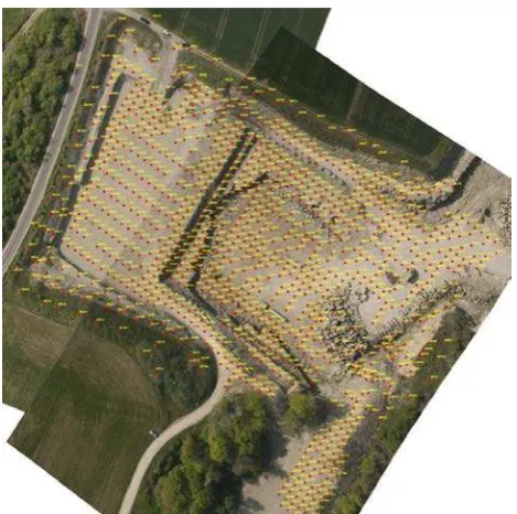
2.2.1. Test field: The test field for this study should contain different geomorphologic landforms, especially those which are difficult to capture by photogrammetric means. A quarry near Trier was chosen to serve as a test field (figure 2), which includes flat areas, several piles of debris and steep faces. A dense and regular network of GCPs was placed across the site to support both, photogrammetric processing as well as the evaluation of the derived DEMs. The GCPs were designed such that they can easily be distinguished from the background and the centre of the GCP can easily be marked during the processing of the aerial images. Altogether 1042 GCPs were distributed and their positions were measured using a Topcon GPT9000a high precision total station.
Figure 2. Quarry serving as test field. Red dots representing the location of 1042 GCPs
2.2.2. Reference data: Altogether, three different datasets were used as reference data for evaluating the DEMs. For the first one (GCP), the coordinates of the GCPs, used for photogrammetric processing of the aerial images, served as reference data, too. Because the GCPs are regularly distributed in the field, this data is very useful for the following accuracy assessment. Due to the fact that the GCPs are installed at even locations, this reference data did not allow evaluating geomorphological complex areas. This led to the preparation of a second reference dataset by measuring about 2000 additional coordinates (HI). These were chosen at positions of high relief energy in order to get a higher density of reference measurements at complex locations. The weakness of this approach lies in the density of measurements which is very heterogeneous over the whole test area. The third reference is an airborne LiDAR dataset flown ten days before the image
has the advantage of a high density of reference measurements across the complete test field.
2.2.3. Image acquisition: The flight path was predefined in GIS-like UAV control software and transferred to the UAV using a wireless connection. The route was designed in wind direction, so that when flying against the wind, very slow aboveground speeds could be achieved. This helped to avoid motion blur due to the conventional high flying speed of the UAV.
The slow above-ground speed has another advantage for image acquisition. Due to the low trigger frequency of the camera, it was not possible to capture the whole area with a 60% of overlap in one flight, flying at low altitudes. To compensate these gaps in the imagery, the flying speed had to be reduced as much as possible and multiple flights at the same flight altitude had to be done, to acquire a complete dataset with overlapping images.
Another issue concerned the presence of shadows. If the image acquisition took too long, the shadows in the images moved due to the motion of the sun, which may negatively impact on the performance of matching algorithms.
In total, 19 flights were performed at different altitudes, ranging from 50m to 550m. 413 of these were chosen to be considered in the following steps.
3. PHOTOGRAMMETRIC PROCESSING
3.1. Aerotriangulation
In order to evaluate the accuracy’s dependency on the number of GCPs used during indirect sensor orientation, six images of different acquisition altitudes were chosen to perform this analysis. During that test, the number of GCPs used during aerotriangulation varied from 3 to the maximum of GCPs that were visible in the image. For every number of control points the sensor orientation has been executed and the RMSE as well as the accuracy of the calculated orientation parameters were registered.
3.2. DEM generation
To maintain the feasibility of the project, not all the possible combinations of image pairs could be processed. Due to the fact that the UAV used for image acquisition didn’t register the exterior orientation (EO) parameters for every captured image, it was necessary to perform a first sensor orientation for the whole dataset. To achieve this, the aerotriangulation was calculated using 5 – 10 GCPs for each of the 413 images. Next, in order to retain a wide variability of parameters like flying altitude, deviation from nadir-view, length of the photo base, etc., 133 image pairs were selected, covering the whole range of these variables. After this selection, the image pairs were processed in Leica Photogrammetry Suite 9.3 (LPS).
The second dataset was generated similarly to the first dataset, except that the algorithms were applied to the first, blue, image channel (dataset 2).
The third set of DEMs was generated using the green channel of the images, too, but in comparison to the first two datasets, the coordinates used to perform the aerotriangulation were reduced in accuracy by adding random noise. This was done to simulate coordinates of GCPs measured by GPS (dataset 3).
All the DEMs were saved in raster format with a ground sampling distance of 5 cm.
3.3. DEM evaluation
3.3.1. Aerotriangulation: The first investigation done using the acquired imagery dealt with the accuracy of the indirect sensor orientation, depending on the number of control points. For that, the exterior orientation parameters for different aerial images were calculated using different amounts and combinations of GCPs. On the one side, the software used to perform this operation, LPS, calculated a RMSE for the whole image block, which in this case contained one sole image. On the other side, an accuracy value for the different EO-parameters was calculated. Both, RMSE and the accuracy values were considered for evaluating the accuracy of the aerotriangulation.
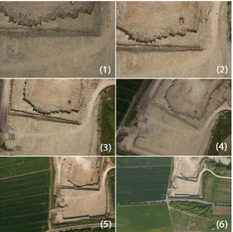
Figure 3. Aerial images of different flight altitudes used for quantification of the indirect sensor orientation accuracy (1: 70m, 2: 100m, 3: 150m, 4: 200m, 5: 300m, 6: 550m)
3.3.2. DEM accuracy: The accuracy of the DEMs was determined by comparing the modeled height values to three different reference datasets. For every DEM, the pixel values were determined at exactly the same coordinates as the points of the reference dataset. Subsequently the differences in height were calculated. Using these residuals a method had to be found to generate an index, describing the accuracy of the DEMs. For every DEM that had to be evaluated, the RMSE and standard deviation (stdv) were calculated from the residuals. These values were used for the following analysis (Haala, 2010).
4. RESULTS AND DISCUSSION
4.1. Aerotriangulation
The first question that was discussed was the quality of the indirect sensor orientation as a function of the number of GCPs which were considered during the aerotriangulation. To get a first impression of the data, the two different values describing the quality of the sensor orientation were plotted against the number of GCPs. Figures 4 and 5 show the results for one aerial image taken at a flight altitude of 300m.
0 200 400 600
Figure 4. RMSE in relation to the number of GCPs used; the red line represents the mean value
0 20 40 60 80 100 120
Figure 5. EO accuracy in dependence of the number of GCPs. Z-component taken as an example
These results confirm the assumption that the accuracy of an indirect sensor orientation increases with a higher number of GCPs considered during the aerotriangulation.
0 100 200 300 400 500 600
Figure 6. Mean EO accuracy for Z-component. Accuracy is decreasing with increasing flight altitude. The five remaining
EO parameters behave similar
Although a higher number of GCPs would improve the accuracy of the sensor orientation and also the quality of the following image processing steps, the number of GCPs was limited to 5 per image. This was decided to maintain the conditions of image acquisition during a field campaign, where the time for preparing the field is limited.
4.2. DEM accuracy
To get an initial impression and overview over the generated data, a scatterplot matrix was visualized. Particular attention was paid to the scatterplots which set the two error values, standard deviation (stdv) and RMSE, in relation to the parameters that could be influenced during image acquisition. Only the flight altitude seemed to show an influence on the accuracy of the DEMs. The remaining parameters showed a randomly distributed point cloud.
Figure 7. Scatterplot matrix showing the relationship between the error values RMSE and stdv against different parameters. Zs1: flight altitude, DZs: difference in flight altitude, DKappa:
In the next step, a linear model was fitted to these point clouds, setting the error values in relation to the image acquisition altitude. A quadratic growth with increasing flight altitude seemed to give the best fit. Figure 7 shows that the two error values, RMSE and stdv, hardly differ. As a consequence, only the RMSE error value is taken into account in the following evaluation.
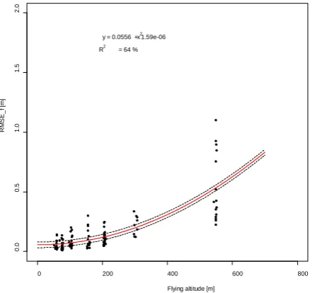
Figures 8, 9 and 10 show the results for dataset 2 (matching algorithms applied on the blue channel). It is important to note, that, comparing with the GCP reference, the spread is minimal but increasing with high flying altitudes.
0 200 400 600 800
Figure 8. Scatterplot setting the residuals’ RMSE (determined with GCP reference) in relation to the flight altitude. The red line represents the linear fit using a quadratic growth; the dotted
line represents the 95% confidence interval.
0 200 400 600 800
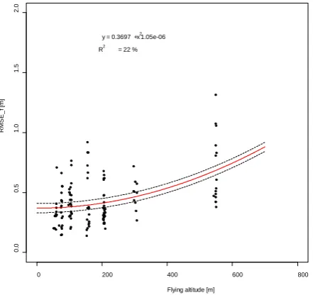
Figure 9. RMSE (determined with HI reference) in relation to the flight altitude.
pictures had to be taken to cover the whole quarry. This was very time consuming and allowed the movement of the shadows. These errors can easily be identified at the portion of low flight altitudes of the figure, which embodies some high error values at 50-70m of flying altitudes. This problem mainly appears in the low flying altitudes, because in that case the movement distance of the shadows easily reaches the distance of the ground sampling distance. As a result the spread is more or less decreasing from low to high flight altitudes and maximal compared to the two plots using the other reference datasets.
For the evaluation using the LiDAR reference, the error values lie somewhere in between of those calculated using the GCP and HI references. The spread is more or less constant for all flying altitudes and intermediate to the two other reference datasets.
Figure 10. RMSE (determined with LiDAR reference) in relation to the flight altitude.
The two remaining datasets behave similarly concerning shape and relative positions of the fitted functions. Table 1 summarizes the equations of the linear fit as well as the coefficients of determination. It is easy to see that using the blue or green channel of the imagery algorithms hardly makes a difference in quality of the generated DEMs.
Dataset Reference Equation R2
1 GCP y = 0.0558+1.59e-06x2 64 %
Table 1. Equation of the linear fit and coefficient of determination for the nine different combinations of DEM- and
reference datasets. Abbreviations explained in the text.
5. CONCLUSIONS
Concluding, a higher number of GCPs considered during aerotriangulation has been shown to improve the quality of the sensor orientation. Unfortunately, the preparations in the field is very time consuming and not feasible for large areas.
In addition, the assumption that using the green channel of an RGB image would improve the quality of the generated DEMs could not be validated, since the differences lie in the range of tenth of millimeters to millimeters.
A final suggestion for application of UAV-photogrammetry, as a method to capture three dimensional data, would be that a compromise has to be found between high resolution and the susceptibility to outliers as a reaction to shadow movement. If high resolution digital elevation models have to be generated, the terrain has to be properly prepared with a time consuming placement of GCPs.
REFERENCES
Aber, J.S., Marzolff, I., Ries, J.B. 2010. Small-Format Aerial
Photography. Principles ,techniques and geoscience
applications. Elsevier, Amsterdam. 268 p.
Acevedo-Whitehouse, K., Rocha-Gosselin, A., Gendron, D. 2009. A novel non-invasive tool for disease surveillance of freeranging whales and its relevance to conservation programs.
Animal Conservation.
Haala, N, Hastedt, H.; Wolf, K., Ressl, C., Baltrusch, S. 2010. Digital Photogrammetric Camera Evaluation - Generation of Digital Elevation Models. Photogrammetrie, Fernerkundung,
Geoinformation, 2/2010, pp. 99-116.
Marzolff, I., Poesen, J. 2009. The potential of 3D gully monitoring with GIS using high resolution aerial photography and a digital photogrammetry system. Geomorphology, 111 (1-2). pp. 48–60.
Everaerts, J., 2008. The Use of Unmanned Aerial Vehicles for Remote Sensing and Mapping. The International Archives of
the Photogrammetry, Remote Sensing and Spatial Information Sciences, Beijing, China. Vol. XXXVII, Part B5, pp.