EVALUATION OF ASTER GDEM V3 USING ICESAT LASER ALTIMETRY
C. C. Carabajal a, J.-P. Boy b
a
Sigma Space Corporation @ NASA/GSFC, Planetary Geodynamics Laboratory – Code 698, Greenbelt, MD 20771, USA - [email protected]
b
EOST/IPGS (UMR 7516 Université de Strasbourg / CNRS), 5 rue René Descartes, 67084 Strasbourg, France - [email protected]
Commission IV, WG IV/3
KEY WORDS: ASTER, ICESat, Topography, Elevation Models, Geodetic Ground Control, Laser Altimetry.
ABSTRACT:
We have used a set of Ground Control Points (GCPs) derived from altimetry measurements from the Ice, Cloud and land Elevation Satellite (ICESat) to evaluate the quality of the 30 m posting ASTER (Advanced Spaceborne Thermal Emission and Reflection Radiometer) Global Digital Elevation Model (GDEM) V3 elevation products produced by NASA/METI for Greenland and Antarctica. These data represent the highest quality globally distributed altimetry measurements that can be used for geodetic ground control, selected by applying rigorous editing criteria, useful at high latitudes, where other topographic control is scarce. Even if large outliers still remain in all ASTER GDEM V3 data for both, Greenland and Antarctica, they are significantly reduced when editing ASTER by number of scenes (N≥5) included in the elevation processing. For 667,354 GCPs in Greenland, differences show a mean of 13.74 m, a median of -6.37 m, with an RMSE of 109.65 m. For Antarctica, 6,976,703 GCPs show a mean of 0.41 m, with a median of -4.66 m, and a 54.85 m RMSE, displaying smaller means, similar medians, and less scatter than GDEM V2. Mean and median differences between ASTER and ICESat are lower than 10 m, and RMSEs lower than 10 m for Greenland, and 20 m for Antarctica when only 9 to 31 scenes are included.
1. INTRODUCTION 1.1 ICESat data as Geodetic Control
The ICESat mission acquired single-beam, globally distributed laser altimeter profiles between ± 86° using the Geoscience Laser Altimeter Sensor (GLAS) (Zwaly et al., 2002 and Schutz et al., 2005). ICESat footprints are spaced over 170 m along the profiles. Data was collected from February, 2003 to October, 2009, during approximately month long observation periods, three times per year through 2006 and twice per year thereafter. These highly accurate altimetry profiles are a consistently referenced elevation data set with quantified errors. ICESat waveforms represent the vertical distribution of energy reflected within the laser-illuminated area (footprint), and centroid elevations indicate the average elevation (Harding and Carabajal, 2005).
We generated Ground Control Points (GCPs) from ICESat, with sub-decimeter vertical accuracy and better than 10 m horizontal accuracy. Table 1 in Carabajal et al. (2011) lists ICESat observation periods, their timelines, transmit energies and long- arc accuracy estimates from rigorous analysis of instrument calibration and validation schemes using ocean scan maneuvers and cross-overs, and correspond to data processed as Release 31, current at the time of GCPs processing. We estimate that our GCPs are of equivalent accuracy for all the observation periods based on the stringent editing criteria applied to the data. Later releases of the data did not include significant modifications to the elevations provided in the GLA14 products used for this millimeters to a few centimeters will have negligible effects on
the outcome of these types of evaluations, and no re-processing of the GCP database has been done with the most recent ICESat data release.
This database of ICESat GCPs have been previously used to characterize and quantify spatially varying elevation biases in Digital Elevation Models (DEMs), assessing the accuracy of valuable topographic datasets like GMTED2010 (Global Multi-resolution Terrain Elevation Data), developed by the USGS (United States Geological Survey) and NGA (National Geospatial-Intelligence Agency), and previously those produced by sensors like the Shuttle Radar Topography Mission (SRTM) (Carabajal and Harding, 2005 and 2006; Carabajal et al., 2010), and the Advanced Spaceborne Thermal Emission and Reflection Radiometer (ASTER) (ASTER Validation Team 2009 and 2011). In this study, we have analysed the error to end of less than 5 m, indicating the within-footprint relief is low. We also apply editing based on laser beam off-pointing and instrumental parameters, working with mostly nadir-looking data, with negligible saturation. All ICESat elevations were converted to WGS84/EGM96 for these comparisons. We exclude ICESat data identified as returns from water based on the ENVISAT MERIS Globcover land cover classification (Bicheron et al., 2008).
elevation products, such as return saturation, and cloud contamination and data from low energy returns, and they are designed based on the particular application. For the higher latitudes, ICESat tracks followed reference tracks on a repeat track mode. When sufficient data along profiles were available for all the periods, we were able to use overlapping profiles to enhance the efficacy of the editing schemes. We have applied a cloud-clearing procedure that identifies the outliers from overlapping profiles in a iterative manner, looking at the mean and standard deviations of the elevation profiles, and using a threshold of 50 m for Greenland, and 40 m for Antarctica.
Data acquired by Laser 3 were used to evaluate the 30 m posting ASTER GDEM Version 3. The spatial distribution of the ICESat footprint energy was Gaussian and nearly circular, with a diameter of about 50 m at the 1/e2 energy level. We computed ASTER GDEM V3 elevations minus ICESat waveform centroid derived elevations at the footprint location using the nearest-neighbor approach. Positive elevation differences means ASTER is above ICESat.
1.2 ICESat Inter-Period Biases
We estimated ICESat inter-period biases by looking at differences from our global comparisons between SRTM v2 finished products elevation data (Farr et al., 2007; Slater et al., 2006) and ICESat centroid elevations for bare Earth only data based on MODIS Land Cover classifications of 100% bare cover (Hansen et al., 2006).
Figure 1. ICESat Laser 3 Inter-Period biases in meters derived from elevation differences against global SRTM elevations at bare earth locations based on MODIS % bare land cover classification.
Figure 1 shows our estimated inter-period biases for Laser 3 periods. Biases reflect changes in instrument characteristics as it experienced a decay in laser energy through its lifetime. These estimates of inter-period biases are robust. They were derived from global comparisons of approximately one million lidar measurements per ICESat observation period with respect to SRTM in non-vegetated and low relief regions. These biases are applied to the ICESat data before computing the differences with ASTER elevation.
2. COMPARISON BETWEEN ASTER AND ICESAT ELEVATIONS IN GREENLAND AND ANTARCTICA 2.1 Comparisons Using all GCP Data
The edited altimetry control is less available around the edges of the ice sheets; nevertheless we have a large number of data available for this comparison. Tables 1 and 2 show the statistics for differences between ASTER GDEM V3 data and all ICESat GCPs, and those obtained when grouping the data based on various categories of number of scenes for Greenland and Antarctica, respectively.
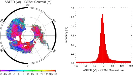
Larger mostly positive elevation differences are seen in the interior of the Greenland ice sheet. The histograms show a tailed distribution skewed toward large positive differences. Smaller differences are observed on the edges, on the order of
For Greenland, differences computed for all GCPs available show a large positive mean elevation difference of 214.90 m, with a median of 85.81 m and an RMSE of 564.17 m, indicating that a large quantity of the data are significantly above the ICESat ground elevations, with extreme outliers.
N scenes N shots Mean (m) Median Greenland. Negative number of scenes corresponds to other elevation sources used for fill.
For Antarctica, differences computed for all GCPs available show a large positive mean elevation difference of 135.42 m, with a median of 0.83 m, and a large 682.12 m RMSE. Comparisons for all GCPs in Antarctica show large negative and positive differences in the Western and Central Antarctica. The frequency distribution is more symmetrical, with a small negative median. On the margins, we observe differences above ±20 m, larger than on the Greenland margins, extending further towards the interior of the ice sheet where the data is available.
N scenes N shots Mean (m)
Median (m)
RMSE (m)
Maximum (m)
Minimum (m)
All 30196718 135.42 0.83 682.12 6161.89 -4049.18
0≤ N <5 22854965 178.92 17.48 783.48 6161.89 -4049.18
5≤ N <9 3704445 5.28 -3.29 73.39 3322.17 -3514.75
9≤ N <16 2294584 -4.38 -5.03 18.86 978.63 -1782.71
16≤ N <31 952768 -6.80 -7.04 15.13 270.21 -1509.33
N ≥ 31 389956 -7.74 -8.08 10.60 148.04 -1066.91
Table 2. Statistics for the ASTER GDEM V3 – ICESat (centroid) elevation differences (in meters) using data from the L3 laser periods as a function of the number of scenes (N) for Antarctica.
2.2 ASTER Along ICESat Elevation Profiles
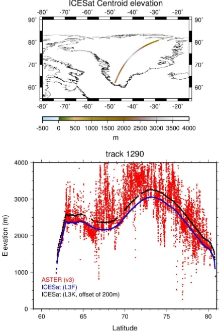
Data from ASTER GDEM elevations extracted at the footprint locations along ICESat profiles show a large degree of scatter. In contrast, the data collected along an ICESat profile shows the larger precision of these elevation measurements for all acquisition periods. Figure 4 shows the ASTER GDEM V3 data for the L3F track across Greenland. The Greenland ice sheet occupies a basin in the central regions, with bedrock surface near sea level under most of Greenland, sometimes exposed along the edges. Two ICESat profiles for observation periods L3F (May, 2006) and L3K (October, 2008) are also plotted, L3K plotted with an offset of 200 m, to better emphasize their agreement.
Figure 4. Elevation data from ASTER GDEM V3 (red) extracted along an ICESat L3F laser altimetry profile for Track 1290 (blue). A profile for L3K offset by 200 m is shown in black.
For Greenland, ASTER GDEM V3 elevations are largely higher with respect to the ICESat elevations, reaching several hundreds of meters above the ground profiles. This agrees with the map
shown in Figure 1. The scatter is reduced at the edges of the profiles. There is a good repeatability along the profiles for the edited ICESat GCP data from the different campaigns.
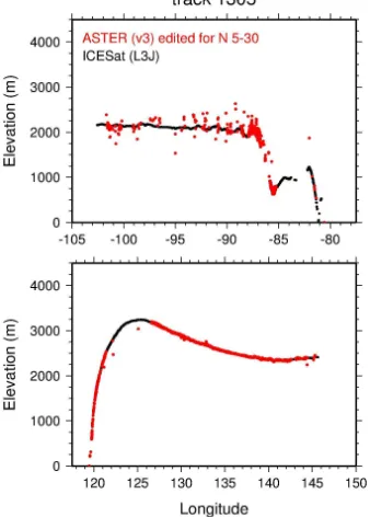
Figure 5. Elevation data from ASTER GDEM V3 (red) extracted along an ICESat L3J laser altimetry profile for two segments of Track 1305 (blue). A profile for L3K offset by 200 m is shown in black.
For Western Antarctica (top profile), ASTER GDEM V3 elevations further inland are several hundred meters than the ICESat elevations, becoming less negatively biased towards the margin. The profile on Eastern Antarctica (bottom profile) shows large negative and positive biases with respect to ICESat, and a close agreement with ICESat in the central region of the profile, with large negative biases towards the interior. This is also in agreement with the observations in Figure 2. As for Greenland, the scatter is reduced at the edges of the Antarctica ice sheet.
3. ELEVATION DIFFERENCES AND NUMBER OF ASTER GDEM V3 SCENES
Multiple ASTER scenes (stereo pairs) are averaged to derive the final GDEM v3 elevation value for any given location using a “stacking” approach (Abrams et al., 2010). To a certain extent, it is expected that the accuracy of the elevation products will increase with the number of scenes used in the production process.
The number of scenes (N) is provided in the ASTER data as an ancillary layer. It represents the number of individual ASTER scenes (stereo pair) DEMs that were stacked and averaged to derive the elevation value at each pixel in ASTER GDEM V3. The number was extracted at each ICESat GCP location, and statistics computed based segmented groupings.
For Greenland, the geographic distribution of N is shown in Figure 6 ASTER is above ICESat when N < 9. For N > 9 the distributions become more normal, with medians closer to the mean differences, and ASTER below ICESat. The smallest means are observed for 9 ≤ N < 16, at -4.06 m, with a median of -7.34 m, and an RMSE of 26.92 m. Less scatter (RMSE = 12.42 m) is observed for 16 ≤ N < 31. When more than 30 scenes are used in the processing of Greenland elevations, the distributions are more symmetrical, with a more negative mean and median of -10.87 and -10.94, respectively, and an RMSE of 12.25 m.
Figure 6. Geographic Distribution of Number of Scenes (N) for Greenland. Negative number of scenes refers to other elevation data used as fill.
Figure 7. Geographic Distribution of Number of Scenes (N) for Antarctica.
For Antarctica, ASTER is above ICESat when N < 9. For N > 9 negative means are observed with ASTER below ICESat, and the distributions become more normal, with medians closer to
the mean differences. The smallest means are observed for 9 ≤ N < 16, at -4.38 m, with a median of -5.03 m, and an RMSE of 18.86 m. For 16 ≤ N < 31, the RMSE is 15.13 m, and the scatter is reduced. When more than 30 scenes are used in the processing of Antarctica, the distributions are more symmetrical, but with a negative mean and median of -7.74 and -8.08, respectively, and an RMSE of 10.60 m, but larger outliers than for Greenland.
3.1 Discriminating by the Number of ASTER GDEM V3 Scenes Used for Processing
Mean elevation differences show the most improvement when 16 to 31 scenes are processed, while minor improvements are achieved in accuracy for N > 16. In our analysis, Figures 8 and 9. We have selected these data processed with more than 5 scenes to examine the effects of editing based on the number of scenes on the quality of the elevation data. The means and standard deviations for the elevations differences are shown in Figures 8 and 9 for Greenland and Antarctica, respectively.
Figure 8. Geographic distribution of 5 ≤ N < 31, frequency distribution, and means, standard deviations and RMSEs for the edited data in Greenland (bottom right).
In both cases, elevation differences for edited data display more normal distributions and a consistent improvement in means and standard deviations as the number of scenes available for processing increases.
m, and an RMSE of 106.54 m. For Antarctica, the mean bias is 2.42 m, a median of -2.66 m, and an RMSE of 52.86 m using 5,334,329 GCPs. In comparison, GDEM V3 for 667,354 GCPs in Greenland show a mean of 13.74 m, a median of -6.37, with an RMSE of 109.65 m. For Antarctica, 6,976,703 GCPs show a mean of 0.41 m, with a median of -4.66 m, and a 54.85 m RMSE. Smaller means, similar medians, and less scatter is observed for GDEM V3.
Figure 9. Geographic distribution of 5 ≤ N < 31, frequency distribution, and means, standard deviations and RMSEs for the edited data in Antarctica (bottom right).
Not all scatter in the ASTER elevations is eliminated when editing by number of scenes, as illustrated by the plots along ICESat profiles shown in Figures 12 and 13, for Greenland and Antarctica, respectively (same geographic location as in the map on the top of Figures 4 and 5). In general, closer correspondence between ASTER and ICESat elevations is observed in the ice sheet margins for Greenland, and in Eastern Antarctica, while the Western Antarctica profile shows that a larger amount of scatter in the elevations still remains.
Figure 10. Geographic distribution of ASTER GDEM V3 minus ICESat elevation differences (top) for edited data (5 ≤ N < 31) and their frequency distribution (bottom) in Greenland, corresponding to the statistics displayed in Figure 8.
Figure 12. ASTER GDEM V3 edited profile (5≤ N <31) across the ICESat L3F profile (track 1290) in Greenland (see Figure 4 for the location on the map).
Figure 13. ASTER GDEM V3 edited profile (5≤ N <31) across the ICESat L3J profile (track 1305) in Antarctica (see Figure 5 for the location on the map).
4. ASTER GDEM V3 AND ICESAT ELEVATION DIFFERENCES WITH RESPECT TO ELEVATION 4.1 Greenland ASTER – ICESat Differences with respect to Elevation
Elevations in Greenland range from elevation at sea level to 3,6694 m (summit of Gunnbjørn Fjeld). Coincidentally, a large portion of the edited data is located in these regions, showing evidence of cloud contamination. For edited ASTER GDEM V3 data (5 ≤ N < 31), geographic distributions of elevations are shown in Figure 14. The highest elevations are located towards the center of the ice sheet, and are between 1,100 m and 1,600 m. The distribution of means and standard deviations show an almost constant negative mean, up to 1,200 m, and a positive mean bias exponentially increasing with respect to increasing elevation, while the standard deviations and RMSEs decrease significantly, showing an exponential increase with elevation
for the higher terrain, and a larger amount of departure from a mean distribution. Statistics are shown in Table 3.
Figure 14. Map of ASTER GDEM V3 minus ICESat GCPs elevation differences (in meters) for Greenland (top). Frequency distribution for data binned at 250 m (center), and means standard deviations and RMSEs of the differences (bottom).
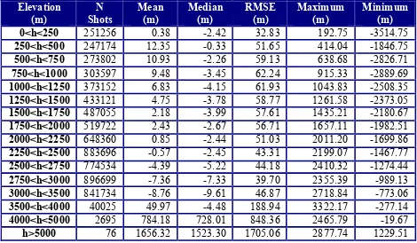
Table 3. Statistics of the edited ASTER GDEM V3 – ICESat (centroid) elevation differences (in meters) for GCPs from L3 periods with respect to elevation, using 250 m ranges, for data in Greenland (5< N <31).
The lowest mean elevations differences are for ranges between 1,250 m and 500 m (139,268 GCPs), with a mean of -0.34 m, a median of -5.69 m and an RMSE of 37.28 m (Table 3). The lowest median elevation of 0.01 m is observed for elevation
Elevation (m) N
Shots Mean
(m)
Median (m)
RMSE (m)
Maximum (m)
ranges between 1,750 m and 2,000 m (67,502 GCPs), with a positive mean elevation difference of 22.41 m, and an RMSE of 78.06 m.
4.2 Antarctica ASTER – ICESat Differences with respect to Elevation
Figure 15. Map of ASTER GDEM V3 minus ICESat GCPs elevation differences (in meters) for Antarctica (top). Frequency distribution for data binned at 250 m (center), and means standard deviations and RMSEs of the differences (bottom).
The highest elevation in Antarctica is Vinson Massif, at 4,897 m, not sampled by the edited data. The lowest mean elevation difference of -0.57 m is seen for elevation ranges between 2,250 m and 2,500 m, with a median of -2.45 m and a 43.31 m RMSE
Accurate global topographic control provided by ICESat has helped establish the accuracy of DEMs and the spatial distribution of elevation biases. These distributions can vary significantly based on the technology used to acquire them and their production method. ASTER requires adequate seasonal illumination for imaging. In stereo methods, smooth terrain complicates scene-pair correlations required to measure terrain height. ASTER GDEM V2 (Tachikawa et al., 2011; Meyer et al., 2012) was developed to address limitations with ASTER GDEM V1 was widely acknowledged as a research grade product with known artifacts (ASTER GDEM Validation Team, 2009). ASTER GDEM V2 represented a marked improvement over its predecessor, including more coverage, improved spatial resolution and better water masking (ASTER GDEM Validation Team, 2011; Meyer et al., 2012).
It is clear that in the ASTER GDEM V3 products some artifacts remain. They are correlated with the number of scenes used in the elevation products, and issues related to cloud masking. Over the ice sheets, larger mean errors are observed. Our assessments indicate that when the data is filtered to exclude areas with perennial ice and/or lacking sufficient observations for correlation (less than 5 scenes), those errors are reduced.
Based on the comparisons against quality ICESat laser altimetry derived GCP elevations where coincident data exists, and our comparable assessments of previous versions of ASTER GDEM as reported in previous Validation Team reports, we conclude that ASTER V3 shows limited improvements over its previous version in Greenland and Antarctica.
Laser altimetry geodetic control data has been proven to provide an adequate means to evaluate the quality of topographic assets. Datasets that include ICESat altimetry as control in their production processing are of superior quality, and efforts to produce global elevation products those types of products are underway. With the upcoming launch of ICESat-2 in late 2017 (Abdalati et al., 2010), and its increased coverage, a vast dataset of global laser altimetry data with which to perform similar assessments, as those pioneered by these techniques.
Elevation
4000<h<5000 2695 784.18 728.01 848.36 2465.79 -19.67
ACKNOWLEDGEMENTS
The development of the ICESat Geodetic Control Data Base was supported by NASA’s Earth Surface and Interior (ESI) Program, Contract NNH09CF42C: “Building an ICESat Geodetic Control Data Base for Global Topographic Mapping and Solid Earth Studies.” David J. Harding was the Co-I in the project, and Vijay P. Suchdeo helped with the pre-processing of the ICESat altimetry before GCP production.
REFERENCES
Abdalati, W., H.J. Zwally, R. Bindschadler, B. Csatho, S. L. Farrell, H.A. Fricker, D. Harding, R. Kwok, M. Lefsky, T. Markus, A. Marshak, T. Neumann, S. Palm, B. Schutz, B. Smith, J. Spinhirne, and C. Webb, 2010. The ICESat-2 Laser Altimetry Mission, Proceedings of the IEEE, Vol. 98, No. 5, pp. 735-751.
Abrams, M., B. Bailey, H. Tsu and M. Hato, 2010. The ASTER global DEM. Photogrammetric Engineering and Remote Sensing, 76, pp. 344–348.
ASTER GDEM Validation Team, 2009. ASTER Global DEM Validation Summary Report (28 p.)
https://lpdaac.usgs.gov/sites/default/files/public/aster/docs/AST ER_GDEM_Validation_Summary_Report.pdf (April 16, 2016).
ASTER GDEM Validation Team, 2011. ASTER Global Digital Elevation Model Version 2 - Summary of Validation Results. (26 p.)
http://www.jspacesystems.or.jp/ersdac/GDEM/ver2Validation/S ummary_GDEM2_validation_report_final.pdf (April16, 2016).
Bicheron P. et al., 2008. GLOBCOVER Products Description and Validation Report, ESA/ESA Globcover Project,MEDIAS France/POSTEL (47 p.)
http://due.esrin.esa.int/files/GLOBCOVER_Products_Descripti on_Validation_Report_I2.1.pdf(April 04, 2016).
Borsa, A. A., G. Moholdt, H. A. Fricker, and K. M. Brunt, 2014. A range correction for ICESat and its potential impact on ice-sheet mass balance studies, The Cryosphere, 8, pp. 345–357.
Carabajal, C.C., and D. J. Harding, 2005. ICESat validation of SRTM C-band digital elevation models, Geophys. Res. Let.,32, L22S01.
Carabajal, C.C. and D. J. Harding, 2006. SRTM C-band and ICESat Laser Altimetry Elevation Comparisons as a Function of Tree Cover and Relief, Photogram. Eng. and Rem. Sens., 72(3), pp. 287-298.
Carabajal, C.C., D.J. Harding and V.P. Suchdeo, 2010. ICESat Lidar and Global Digital Elevation Models: Applications to DESDynI, Geoscience and Remote Sensing Symposium (IGARSS), 2010 IEEE International, Honolulu, HI, pp. 1907-1910.
Carabajal, C.C., D.J. Harding, J.-P. Boy, J.J. Danielson, D.B. Gesch and V.P. Suchdeo, 2011. Evaluation of the Global Multi-Resolution Terrain Elevation Data 2010 (GMTED2010) Using ICESat Geodetic Control, SPIE Proceedings, International Symposium on LIDAR and Radar Mapping: Technologies and Applications (LIDAR & RADAR 2011), Nanjing, China.
Farr, T.G., P. A. Rosen, E. Caro, R. Crippen, R. Duren, S. Hensley, M. Kobrick, M. Paller, E. Rodriguez, L. Roth, D. Seal, S. Shaffer, J. Shimada, J. Umland, M. Werner, M. Oskin, D. Burbank and D. Alsdorf, 2007. The Shuttle Radar Topography Mission. Reviews of Geophysics, 45(RG2004.
Hansen, M., R. DeFries, J.R. Townshend, M. Carroll, C. Dimiceli, and R. Sohlberg, 2006. Vegetation Continuous Fields MOD44B, 2001 Percent Tree Cover, Collection 4, University of Maryland, College Park, Maryland, 2001.
Harding, D.J., and C.C. Carabajal,, 2005. ICESat Waveform Measurements of Within-footprint Topographic Relief and Vegetation Vertical Structure, Gephys. Res. Lett., L21S10.
Meyer, D.J., Tachikawa, T., Abrams, M., Crippen, R., Krieger, T., Gesch, D., et al., 2012. Summary of the validation of the second version of the aster GDEM. 2012 XXII ISPRS Congress
(pp. 291–293). Melbourne, Australia: ISPRS.
Schutz, B.E., H.J. Zwally, C.A. Shuman, D. Hancock, and J.P. DiMarzio, 2005. Overview of the ICESat Mission, Geophys. Res. Lett., 32, L21S01.
Slater, J.A., G. Garvey, C. Johnston, J. Haase, B. Heady, G. Kroenung and J. Little, 2006. The SRTM Data Finishing Process and Products, Photogrammetric Engineering and Remote Sensing,. 772(3), pp. 237-248.
Tachikawa, T., M. Hato, M. Kaku and A. Iwasaki, 2011. Characteristics of ASTER GDEM version 2. Geoscience and Remote Sensing Symposium (IGARSS), 2011 IEEE International, Vancouver, BC, 2011, pp. 3657-3660.