MULTI-TARGET DETECTION FROM FULL-WAVEFORM AIRBORNE LASER
SCANNER USING PHD FILTER
T. Fuse a, D. Hiramatsu a, W. Nakanishi a, *
a Dept. of Civil Engineering, The University of Tokyo, 7-3-1 Hongo, Bunkyo-ku, Tokyo 1138656 Japan - (fuse@civil, hiramatsu@trip, nakanishi@civil).t.u-tokyo.ac.jp
Commission V, WG V/4
KEY WORDS: Probability hypothesis density, Full-waveform airborne laser scanner, Multi-target detection
ABSTRACT:
We propose a new technique to detect multiple targets from full-waveform airborne laser scanner. We introduce probability hypothesis density (PHD) filter, a type of Bayesian filtering, by which we can estimate the number of targets and their positions simultaneously. PHD filter overcomes some limitations of conventional Gaussian decomposition method; PHD filter doesn’t require a priori knowledge on the number of targets, assumption of parametric form of the intensity distribution. In addition, it can take a similarity between successive irradiations into account by modelling relative positions of the same targets spatially. Firstly we explain PHD filter and particle filter implementation to it. Secondly we formulate the multi-target detection problem on PHD filter by modelling components and parameters within it. At last we conducted the experiment on real data of forest and vegetation, and confirmed its ability and accuracy.
* Corresponding author
1. INTRODUCTION
Full-waveform airborne laser scanner becomes widely used in LiDAR. Reflection intensity data acquired by full-waveform airborne laser scanner is expected to be useful compared with traditional discrete-return laser system, especially in the case multiple target exist above ground. For example, to retrieve 3D canopy structure from LiDAR data is important with regard to carbon cycle modelling (Hurtt et al., 2004). Many researchers have used Gaussian decomposition to model and analyse full-waveform data, and detect multiple targets including ground (e.g. Persson et al., 2005; Wanger et al., 2006; Pirotti, 2011). However it is difficult to detect multi-target precisely when reflection intensity from target is weak and not distinguishable from noise. Richter et al. (2014) has proposed the method to correct attenuation reflected by target which are further from scanner. Nevertheless, the two shortcomings with Gaussian decomposition are the following; we have to fix the number of targets in advance, and the reflection intensity might not fit Gaussian distribution.
As discussed in Kleinherenbrink et al. (2014), the reflection intensity of successive signals can be helpful in specifying targets, for the signals are continuous spatially and temporally. Based on this concept of similarity in reflection intensity distribution of neighbourhood signals, we regard the multi-target detection problem as the time-series analysis. We propose a new method of analysing the full-waveform data for multi-target detection by employing probability hypothesis density (PHD) filter. PHD filter is a type of Bayesian filter; Bayesian update system of PHD introduced by Mahler (Mahler, 2000; Mahler, 2003). PHD filter is applied to multi-target tracking, for it can deal with unknown and variable number of objects. More specifically we can estimate the number of targets within the area and their positions simultaneously by PHD filter. In fact,
many applications of PHD filter to multi-target tracking have shown that the filter is a robust solution to deal with uncertain factors such as number of targets and accuracy of observation (e.g. Tobias and Lanterman, 2004; Ikoma et al., 2008).
Our idea is that the problem of variable-number multi-target tracking by still sensor is similar to the problem of variable-number multi-target detection by moving sensor, e.g. aerial laser scanner. The structure of these problems are almost the same; what we can observe are generated stochastically by latent variables, or “state”, and state follows a certain dynamics and it sometimes appears and disappears. What generates time-series changing is the only difference; in tracking, motion of target does, and in detection, irradiation angle of sensor. In the following section, we explain PHD filter, formulate multi-target detection problem by using it, and then apply a proposed method to the acquired data of forest and vegetation.
2. PROBABILITY HYPOTHESIS DENSITY FILTER
2.1 Sequential Bayesian Filtering
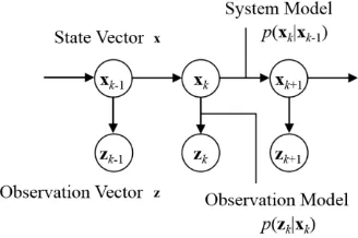
Consider a general state space model (Figure 1): non-Gaussian and nonlinear state space model for time series zk,
1 | k p k k
x x x (1)
zk p
zk|xk
(2)where xk is an unknown state vector and the conditional probability functions of each equation are not necessarily Gaussian. Equation (1) is called the system model and equation (2) the observation model. After we obtain z1:k = {z1, z2,..., zk},
a series of observations from time 1 to k, the posterior distribution of xk is calculated by Bayes’ theorem as follows:
1: 1: 1
Equation (3) shows the process of sequential Bayesian filtering. It includes the system model and the observation model, and the estimated result at time k-1: p(xk-1|z1:k-1). Therefore we can sequentially estimate the posterior of xk by this equation. If we need the estimated value for xt, an expected value of p(zt|xt) is usually used.
Figure 1. General state space model
2.2 PHD Filter
Equation (3) can be directly applied to the single- or constant-number-target detection. However, considering a variable- number multi-target detection, the dimension of xk should increase or decrease appropriately according to the increase or the decrease of targets. Thus equation (3) cannot be directly used for problems in such situations, which are indeed true with real application.
Consider a random and non-negative integer n(k), the number of targets at time k, and a state vector Xk ={x1, x2,…,xn(k)} at time k. As n(k) is stochastic, Xk is also a random variable (vector). Usually state space of Xk is not computable because its dimension increases exponentially according to the number of objects. Instead, probability hypothesis density (PHD), the first order moment of this state space is proposed. And PHD is shown to be identical to the factorial moment density in point process theory, so PHD can be any density function that when integrated over the interested area, the integration of it is the expected number of the targets within that area. Therefore taking multi-target detection as an example, under a set of time-series observations Z1:k = {Z1, Z2,…, Zk} from sensors, we can estimate the number of targets n(k) and their positon xk at time k: Xk ={x1, x2,…,xn(k)} by PHD filter.
We indicate PHD of a state vector x as D(x). Then the predictive PHD at time k given observation from time 1 to k-1 is described as
k| 1:k1
s
k| k1
k1| 1:k1
k1 birth
kD x Z p
p x x D x Z dx D x (4)where ps is the survival probability that the target x at time k-1 will appear at k, Dbirth(xk) is the PHD of the likelihood function that makes a new targets x at time k, and p(xk|xk-1) is the single-target motion model: system model of equation (1). Then the posterior of PHD after observation at time k is that
observation model of equation (2): the conditional probability density of observation z given x.
The integration of posterior of PHD (equation (5)) is the expectation of the number of targets at time k, n(k). That is,
k| 1:k
kE n k
D x Z dx (6)and usually we use the nearest integer of E[n(k)] as the estimated value of number of targets at time k.
2.3 Particle Filter Implementation of PHD Filter
In this subsection, we explain how to calculate equation (4) and (5) using particle approximation (Figure 3). This implementation has been proposed by some researchers (Vo et al., 2003; Zajic and Mahler, 2003; Vo et al., 2005).
2.3.1 Preparation: Consider a set of particles
that approximates the PHD at time instance k-1, where xk-1,i is a realisation of D(xk-1), wi is the weight of particle i, and Lk-1 is the number of particles and at time k-1. Set the number of particles ρ par one object. Then Lk-1 = ρ×E[n(k-1)] and wi = 1/ρ.
2.3.2 System Model: Firstly calculate the first term of right-hand member of equation (4) by set wi = ps/ρ:
This calculation corresponds to the survival of the target. Then calculate the second term of right-hand member of equation (4) by generate ρ particles drawn from Dbirth(xk) with their weight
Then we obtain the particle approximation of posterior PHD at time instance k as
2.3.4 Estimation and Resampling: Calculate equation (6) as
i iE n k
w (11)and the number of particles to be resampled as
k i
i
L
w (12)Then resample particles by drawing Lk times from the posterior PHD: the probability of each particle proportional to its weight. Now we obtain equation (7) at time k, and then repeat from 2.3.2.
Figure 2. Particle filter implementation of PHD filter
3. PHD FILTERING FORMULATION FOR MULTI-TARGET DETECTION
In this section we formulate the multi-target detection problem using PHD filter.
3.1 Observation
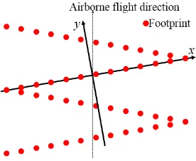
Firstly we explain the data and observations. Full-waveform laser scanner records the reflection intensity as a function of elapsed time, or time of flight, t from the laser irradiation at time k (Figure 3). A peak of high intensity implies that there is a target (Figure 4). And we can calculate the distance between the scanner and each reflection point using the speed of light c, the relative position using the irradiation angle θ. However there can be a target even if the intensity has only a weak peak. So the problem is how to identify the number of target from the waveform information by relating the peak of intensity to the target and distinguishing them from noise, at each irradiation.
3.2 Formulation
3.2.1 State Vector and Observation Vector: We consider a simple situation that we have known the height and attitude of airborne. Also since the scanning rate is high enough, we can assume that the airborne almost remains still and the targets are almost at the same positions in the successive irradiation. Therefore the change of the irradiation angle of the scanner is only considered in the following of this paper. Above these assumptions, we define variable x as position on ground: xy-plane (x, y) and height from scanner h. We also define variable z as a series of reflection intensity r={r1, r2,…, rT}.
3.2.2 System Model: If we consider that the dataset is small and thus define x axis parallel to the scanning line (Figure 5), random error term for each element of x. The equation that hk is approximately equal to hk-1 is based on the high scan rate assumption stated above. And under this assumption, the system model for x is derived as
Figure 4. x-h coordinates, reflection intensity and target
Figure 5. x-y coordinates for small dataset
3.2.3 Observation Model: We can employ any function that relate the observation r and the variable x as an observation model. Note that even in the full-waveform, intensity r is recorded as the convolution of energy in a short time window between t and t+Δt, and we denote it as the intensity rt at discrete time instance t. In this paper, we define the observation model as following model:
and c is the speed of light. The first equation of (16) means that twice of the distance from the scanner to the target equals the elapsed time t* times c, and the second means the interpolation of intensity at t* using neighbour discrete time t. This model represents that higher intensity implies higher likelihood of the existence of the target.
constant p and uniformly distributed D.
3.3 Object Identification
3.3.1 Concept: PHD in equation (4) and (5) doesn’t have any information about the target identification. One possible solution to identify each target from PHD is to apply a clustering method at each time. On the other hand, in case of the PHD filter in this paper, we assume that we can track each target before detection at each time k, namely “track
-before-detect” approach in the field of visual tracking. In this
subsection, we explain the manner to manage labels put on to each target, based on Ikoma et al. (2013). The purpose here is to determine each particle’s association with target to calculate the position of each target.
3.3.2 Modification in Filtering: We put a set of positive integer labels on each target. Thus, we add a label variable l to state vector x of equation (7),
and we put l=0 for newly generated particles. Then the same as Ikoma et al. (2013), based on l at previous time instance k-1, we eliminate other targets from the original reflection signal at time k. We calculate state-dependent likelihoods for each target, instead of summation of all targets in equation (9). The estimation result for each target is calculated as the expected value for each label.
3.3.3 Labelling Rule: After we calculate posterior PHD at time k, we update the set of labels according to labelling rule. It includes putting new label and removing existing label. We put new positive integer label for particles with l=0 if the summation of their weight within a sliding window along h is greater than threshold ladd. In the same way, we remove the existing label with positive integer if the summation of their weight are less than threshold lrem, and replace their labels with l=0. The threshold ladd and lrem are defined in advance. Note that this labelling is independent of PHD estimation itself. Thus the
integration of particles’ weight with a certain label may be
3.3.4 Initial PHD: At last, we manually set the initial PHD, setting variables (x, h, l) for each target. Although this process can be replaced with automatic target detection method, as we focus on basic performance of PHD filtering step in this paper, we give priority to avoiding any initial errors.
4. EXPERIMENTS
4.1 Data and Setting
We use the full-waveform data of forest and vegetation at the Institute for Nature Study located in Tokyo. Data was acquired on October 20, 2012, from the altitude of 950m. Scan rate is 100[kHz], scan rate is 42[Hz] and scan angle is 30[°] (see Nakano and Chikatsu (2015) for more detail). Thus we can calculate ωΔt = 4.4×10⁻⁴[rad/shot] in equation (13) and (14).
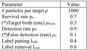
Experiment to detect multi-targets in 20 irradiation points that are align is conducted. We define x axis on this alignment so that we can omit the variable y on xy-plane. Thus we directly use the system and observation model of equation (13) and (15), respectively. According to the data, we set the parameters
(*)Target birth and false detection rate are assumed to follow a uniform distribution over the state-space in this experiment.
Table 6. Parameter settings
4.2 Result and Discussion
Firstly we obtain ground truth data by manually detecting targets from original reflection signals. There are 56 targets during 20 time steps and the number of targets at each time varies from one to four (Figure 7).
Experimental results show that the proposed technique can simultaneously estimate the number of targets and their positions. Figure 7 shows the estimated and true number of targets at each time. Precise estimation is achieved by the
proposed technique at many time instances. It may be a limitation so far that after emergence of new target and disappearance of existing target at around time k=10 and k=16, the estimated number of targets cannot follow such increase or decrease immediately. Nevertheless, after a few time steps, the estimation become precise again.
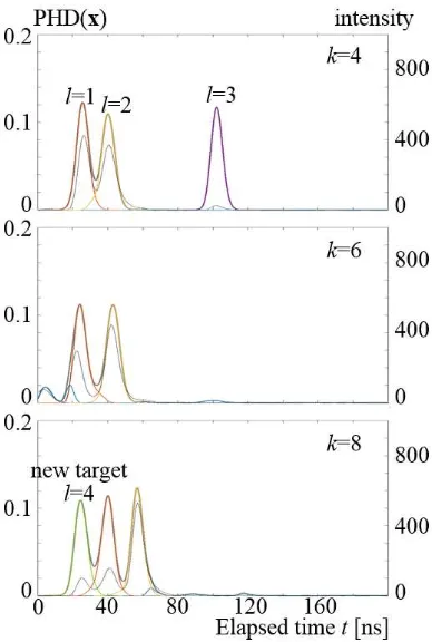
Figure 8 shows the estimated posterior PHD and original reflection signal at some time instances. Colour lines show the PHD corresponding to each target. Red line shows the label variable l=1, yellow l=2, purple l=3, yellow green l=4, and blue l=0. Their densities are shown in left-hand side axis. Also the black line shows the intensity of right-hand side axis. Since the peak of reflection intensity corresponds to peak of PHD, we can conclude that the estimation of position of each target is also almost accurate. Especially the increase and decrease of the number of targets are estimated accurately at time k=6 and k=8.
Figure 9 shows the expected and true value of the position of targets, (x, h). Residuals of estimated position are within 20[cm] for 29 targets of 56, and 50[cm] for 39 targets. Some false detections are shown in Figure 9. For example, one target is incorrectly detected as two targets at k=10, and two targets as only one target at k=16. They will be solved by more accurate observation model and labelling. Precise analysis on the shape of waveform corresponding to existence of targets will be the next step to find such models.
5. CONCLUSION
In this paper, we introduced the technique of PHD filter to multi-target detection by full-waveform airborne laser scanner. We assumed the detection problem as the time series analysis and formulated the filtering model. In the modelling of PHD filter, movement of scanner is modelled as the system model, reflection intensity as the observation model, and increase and decrease of the number of the targets as the birth and survive rate. We also set the rule of labelling to identify each target estimated by the filter.
Experimental result showed the ability of the proposed method to estimate the number of objects and their positions. Besides, compared with existing method, this method allowed an analysis without a priori knowledge of the number of targets and an assumption of Gaussian distribution.
In the future, other observation models need to be employed, which are more robust to noises. For instance, we will consider that the target corresponding to the ground surface has more survival rate than that to the vegetation. Also an application of this method to the problem of larger size such as whole forest is recommended. They will be presented in a future paper. Colour lines show the estimated PHD of each label (left axis) and black shows the signal intensity (right axis).
Elapsed time t can be converted to x-h coordinates by equation (14). Smaller t means smaller h (also see Figure 9) Figure 7. Number of targets at each time k
Figure 9. Estimated results on x-h coordinates Figure 8. Estimated PHD
ACKNOWLEDGEMENTS
The authors would like to thank Aero Asahi Corporation for providing LiDAR data used in this paper.
REFERENCES
Hurtt, G. C., Dubayah, R., Drake, J., Moorcroft, P. R., Pacala, S. W., Blair, J. B. and Fearon, M. G., 2004. Beyond potential vegetation: combining lidar data and a height-structured model for carbon studies. Ecological Applications, 14, pp.873– 883.
Ikoma, N., Yamaguchi, R., Kawano, H. and Maeda, H., 2008. Tracking of Multiple Moving Objects in Dynamic Image of Omni-Directional Camera using PHD Filter. Journal of Advanced Computational Intelligence and Intelligent Informatics, 12(1), pp.16-25.
Ikoma, N., Hasegawa, H. and Haraguchi, Y., 2013. Multi-Target Tracking in Video by SMC-PHD Filter with Elimination of Other Targets and State Dependent Multi-Modal Likelihoods. 16th International Conference on Information Fusion, pp.588-595.
Kleinherenbrink, M., Ditmar, P. G. and Lindenbergh, R. C., 2014. Retracking Cryosat Data in the SARIn Mode and Robust Lake Level Extraction. Remote Sensing of Environment, 152, pp.38-50.
Mahler, R. P., 2000. A Theoretical Foundation for the
Stein-Winter “Probability Hypothesis Density (PHD)” Multitarget
Tracking Approach. Army Research Office, Alexandria VA.
Mahler, R. P., 2003. Multitarget Bayes Filtering via First-Order Multitarget Moments. IEEE Transactions on Aerospace and Electronic Systems, 39(4), pp.1152-1178.
Nakano, K. and Chikatsu, H., 2015. On Ground Surface Extraction Using Full-waveform Airborne Laser Scanner for CIM. ISPRS Archives, 45(4/W5), pp.159-163.
Persson, A., Soderman, U., Topel, J. and Ahlberg, S., 2005. Visualization and Analysis of Full-waveform Airborne Laser Scanner Data. ISPRS Archives, 36(3/W19), pp.103-108.
Pirotti, F., 2011. Analysis of full-waveform LiDAR Data for Forestry Applications: a review of investigations and methods. iForest - Biogeosciences and Forestry, 4(3), pp.100-106.
Richter, K., Stelling, N. and Maas, H. G., 2014. Correcting Attenuation Effects Caused by Interactions in the Forest Canopy in Full-waveform Airborne Laser Scanner Data, ISPRS Archives, 40(3), pp.273-280.
Tobias, M. and Lanterman, A. D., 2004. A Probability Hypothesis Density-based Multitarget Tracker Using Multiple Bistatic Range and Velocity Measurements. IEEE Proceedings of the Thirty-Sixth Southeastern Symposium on System Theory 2004, pp.205-209.
Vo, B. N., Singh, S. and Doucet, A., 2003. Sequential Monte Carlo Implementation of the PHD Filter for Multi-target
Tracking. Proceedings of International Conference on Information Fusion, pp.792-799.
Vo, B. N., Singh, S. and Doucet, A., 2005. Sequential Monte Carlo Methods for Multi-Target Filtering with Random Finite Sets. IEEE Transactions on Aerospace and Electronic Systems, 41(4), pp.1224-1245.
Wagner, W., Ullrich, A., Ducic, V., Melzer, T. and Studnicka, N., 2006. Gaussian Decomposition and Calibration of a Novel Small-footprint Full-waveform Digitising Airborne Laser Scanner. ISPRS Journal of Photogrammetry and Remote Sensing, 60(2), pp.100-112.
Zajic, T. and Mahler, R. P., 2003. A Particle-systems Implementation of the PHD Multitarget-tracking Filter, Proceedings of SPIE 5096, Signal Processing, Sensor Fusion, and Target Recognition XII, pp.291-299.