Investigations on the quality of the interior orientation
and its impact in object space for UAV photogrammetry
H. Hastedt a, *, T. Luhmann a
a IAPG, Jade University of Applied Sciences, Ofener Str. 16/19, 26121 Oldenburg, Germany - (heidi.hastedt, luhmann)@jade-hs.de
KEY WORDS: UAV, interior orientation, accuracy, camera calibration, photogrammetry, Computer Vision, OpenCV
ABSTRACT:
With respect to the usual processing chain in UAV photogrammetry the consideration of the camera’s influencing factors on the accessible accuracy level is of high interest. In most applications consumer cameras are used due to their light weight. They usually allow only for automatic zoom or restricted options in manual modes. The stability and long-term validity of the interior orientation parameters are open to question. Additionally, common aerial flights do not provide adequate images for self-calibration. Nonetheless, processing software include self-calibration based on EXIF information as a standard setting. The subsequent impact of the interior orientation parameters on the reconstruction in object space cannot be neglected. With respect to the suggested key issues different investigations on the quality of interior orientation and its impact in object space are addressed. On the one hand the investigations concentrate on the improvement in accuracy by applying pre-calibrated interior orientation parameters. On the other hand, image configurations are investigated that allow for an adequate self-calibration in UAV photogrammetry. The analyses on the interior orientation focus on the estimation quality of the interior orientation parameters by using volumetric test scenarios as well as planar pattern as they are commonly used in computer vision. This is done by using a Olympus Pen E-PM2 camera and a Canon G1X as representative system cameras. For the analysis of image configurations a simulation based approach is applied. The analyses include investigations on varying principal distance and principal point to evaluate the system’s stability.
1. INTRODUCTION
In UAV photogrammetry the interior orientation of the camera system, its stability during image acquisition and flight as well as its calibration options and consideration in the bundle adjustment, are limiting factors to the accuracy level of the processing chain. In most applications of UAV imagery, consumer cameras are used because of a limited payload, a specific hardware configuration and cost restrictions. In general, such consumer cameras provide automatic zoom, image stabilization and restricted options in manual modes. These issues lead to a lower accuracy potential due to a lack of stability and long-term validity of the interior orientation parameters. Besides the use of accuracy limiting hardware components, the application of different software packages for UAV photogrammetry might significantly influence the processing results. In most cases the application of professional photogrammetric processing software for UAV imagery is limited. This would require standard image blocks due to the determination of overlapping areas for automatic processing as it is usually found within aerial photogrammetry products. UAV imagery is highly influenced by the dynamics during the flight and cause more irregular image blocks and subsequent processing difficulties. Therefore, specialized processing software for UAV photogrammetry is established nowadays. Such software products like Agisoft PhotoScan or Pix4D are mainly based on principles of computer vision, namely structure-from-motion approaches. The consideration of fixed pre-calibrated interior orientation parameters is possible. However, this does usually not shape the standard processing scenario within UAV software that considers a self-calibration and EXIF information for the camera’s initial parameters. Especially a complete photogrammetric camera calibration might not be available for all user groups.
Camera calibration and the evaluation of high-quality interior orientation parameters is one main topic in research and development of photogrammetry since decades (Remondino & Fraser 2006). Within computer vision one can see an increasing interest in the investigations of camera calibration and interior orientation models. Both disciplines use similar strategies in order to get object reconstructions in 3D space by using image based data sets. As a major difference between the two disciplines it can be stated that in photogrammetry accuracy and reliability in object reconstruction including a precise camera calibration is of highest interest whereas in computer vision the scene reconstruction focuses on complete and quick algorithms and systems. A reliable and significant estimation and consideration of the interior orientation parameters is of lower interest and therefore missing in some systems and applications. Nevertheless, both mathematical approaches are based on the central projection. Often the same functional descriptions for the interior orientation, based on Brown (1971), is applied (e.g. OpenCV, iWitness). While a reverse non-linear modelling in 3D space forms the photogrammetric approach (Luhmann 2014), a two-step method based on linear descriptions following Zhang (2000) or Heikkila & Silvén (1997) and subsequent non-linear adjustments can be found in computer vision, which mainly rely on the usage of planar calibration patterns.
Colomina & Molina (2014) give a detailed summary on nowadays UAV systems, techniques, software packages and applications. With respect to the camera’s interior orientation parameters the relevance of their estimation and its impact in object space is rarely analysed or documented. Douterloigne et al. (2009) present a test scenario for camera calibration of UAV cameras based on a chess-board pattern. The repeatability of the interior orientation parameters is evaluated by using different The International Archives of the Photogrammetry, Remote Sensing and Spatial Information Sciences, Volume XL-1/W4, 2015
image blocks and error propagation systems. An extended test on the comparability of camera calibration methods is done by Pérez et al. (2011). Camera calibration results based on an a priori testfield calibration and a field calibration procedure are evaluated with respect to the parameter values and the resulting precision in image space. A subsequent estimation of its impact in object space is done for one scenario. Here the resulting coordinates of the bundle adjustment at defined signalized targets are checked against their GPS coordinates. Cramer et al. (2014) compare results of an on-the-job calibration within UAV applications and their impact in object space by applying a digital surface comparison to reference points. Simulation based scenarios for image block configurations in field calibrations are published by Kruck & Mélykuti (2014). They notice that the simulation focuses on the determinability but not on the reliability of parameter estimation. Different published analyses and applications include approaches to assess the parameters of interior orientation and its influence on the results of specific UAV applications.
Nevertheless the impact of the interior orientation parameters in object space within UAV flight scenarios has to be analysed furthermore. With respect to the suggested key issues different investigations on the quality of interior orientation and its impact in object space are addressed. On the one hand the investigations concentrate on the improvement in accuracy by applying pre-calibrated interior orientation parameters. On the other hand, image configurations are investigated that allow for an adequate self-calibration in UAV photogrammetry.
2. DEFINTION OF INTERIOR ORIENTATION
2.1 Mathematical models of interior orientation
The functional model in photogrammetric reconstruction as well as in computer vision is based on the pinhole camera model or central projection, respectively. Within a self-calibration framework or a previously conducted testfield calibration three groups of parameter sets for modelling the interior orientation of a camera are included in the basic functional model:
a. principal distance c and principal point x'0, y'0
b. radial-symmetric lens distortion (rad) c. decentring distortion (tan).
Usually interior camera parameters are set constant for all images of a photogrammetric project. Distortion parameters are defined with respect to the principal point. Then the standard observation equation in central projection (1) yield
'
The standard observation equation (1) summarizes the effects of distortion (2) through the correction of Δx' in the image space
x-direction, Δy' respectively (Luhmann et al. 2014). For radial-symmetric lens distortion (3) an unbalanced form (4) is chosen. The decentring distortion (also known as radial-asymmetric and tangential distortion) follows equations (5).
tan
The interior orientation model for photogrammetric approaches and those of computer vision, like Agisoft Photoscan or OpenCV is based on Brown (1971). The results are comparable when applying equality of the principal distance and pixel size in x- and y-direction of image space.
Camera modelling with image-variant parameters causes three more parameters per image to be estimated within the bundle adjustment. Hence the number of unknown grows up to nine per image. These parameters describe the variation of the principal distance and the shift of the principal point, hence the possible displacement and rotation of the lens with respect to the image sensor are compensated by this approach using extended standard observation equation (6).
i
2.2 Conversion of interior orientation parameters
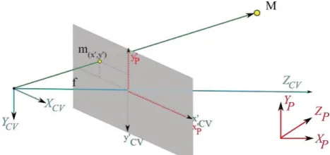
Although the basic functional model is equal between the photogrammetric approach (AXIOS Ax.Ori) and those in computer vision (OpenCV and Agisoft PhotoScan) a parameter conversion is necessary. In order to support a direct comparability of the resulting parameters the implemented functional contexts have to be analysed and conversion terms have to be defined. A major difference can be identified within the definition of the coordinate systems (Figure 1). In computer vision approaches the image space is defined within the pixel coordinate system and its common positive directions. This influences the principal distance as well as the principal point.
Figure 1: Coordinate system definitions
Due to the direct linear imaging description of computer vision approaches the resulting distortion parameters are superimposed by the principal distance when compared to a photogrammetric system. Hastedt (2015) describes the comparability and conversion of parameter groups of interior and exterior orientation. Table 1 summarizes the necessary conversion terms from computer vision results to photogrammetric notation. The International Archives of the Photogrammetry, Remote Sensing and Spatial Information Sciences, Volume XL-1/W4, 2015
Photogrammetry PhotoScan / OpenCV
c[mm] -fx · pixSize [mm] = -fy · pixSize [mm]
x'
0 [mm] (cx-0.5 sensorsize_xpix)·pixelSize [mm] y'
0 [mm] (-cy+0.5 sensorsize_ypix)·pixelSize [mm]
A1 [1/mm²] K1 / cmm²
A2[1/mm4] K2 / cmm4 A3[1/mm6] K3 / cmm6 B1[1/mm2] P2 / cmm2 B2[1/mm2] -P1 / cmm2
Table 1. Conversion scheme of interior orientation
Some approaches in computer vision, like Agisoft PhotoScan, allow for the estimation and consideration of a skew parameter. As this is not comparable to photogrammetric approaches it will not be dealt within these investigations.
3. CAMERA CALIBRATION
3.1 Tested cameras
For UAV photogrammetry a microdrones md4-1000 is used and an Olympus Pen E-PM2 system camera (Figure 2) is equipped to the system. This camera offers a high imaging quality whereas the geometric quality is influenced by different effects and has to be modelled conscientiously. The camera offers an imaging resolution of 4608 x 3456 pixels with a pixel size of 3.75 µm and a 14 – 42 mm zoom lens. The manual mode can be used with manual focus, however the focussing can only be checked in live view and not be fixed at infinity. This limits the usability as the auto-focus needs to be fixed once in order to enable a sharp image acquisition at infinity. Therefore adequate camera settings for flight purposes are limited as the camera settings cannot be changed within the flight in order to support right focussing.
Figure 2. Olympus Pen E-PM2
In addition a Canon G1X system camera is tested for comparison. This camera acquires images with a resolution of 4352 x 2907 pixels. The pixel size is 4.3 µm, the zoom-lens can be used with 15 – 64 mm.
3.2 Test fields and scenarios
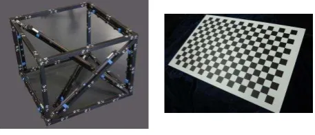
The investigations on the quality of the interior orientation estimation are based on two test scenarios. On the one hand a typical photogrammetric image block (Table 2, top) is taken over a volumetric VDI testfield (VDI 2002, see Figure 3). On the other hand a planar chessboard pattern (Figure 3) is chosen, as it is commonly used within computer vision applications and products. Two different image blocks are taken whereby a
strong block configuration is characterized by an almost volumetric image acquisition around the object including images rolled around the camera axis at each camera station. This enables a reliable and stable parameter estimation. The weak block configuration follows some typical descriptions of camera calibration blocks within computer vision. One can often find a recommended image acquisition by slightly moving the camera in front of the calibration pattern. This leads to more or less random results for the interior orientation parameters. Luhmann et al. (2014) and Hastedt (2015) summarize typical scenarios to circumvent these effects.
Figure 3. Volumetric VDI testfield and planar chess board pattern
Image block taken over a volumetric VDI testfield
volumetric distribution of images
images rolled through the camera axis all around
the scenario
Strong image block taken over a planar chessboard
pattern
almost volumetric distribution of images images rolled around the
camera axis
Weak image block taken over a planar chessboard
pattern
images in front of planar pattern
slightly moved and rolled image positions
Table 2. Image block configurations for camera calibration The International Archives of the Photogrammetry, Remote Sensing and Spatial Information Sciences, Volume XL-1/W4, 2015
VDI - 3D VDI - 3D VDI - 3D
Ax.Ori Agisoft OCV Ax.Ori Agisoft OCV Agisoft OCV Ax.Ori Agisoft OCV
c [mm] 15.3804 15.3417 15.4139 14.5060 14.4967 14.5538 14.5202 14.6537 14.5027 14.4735 14.5379
dev. to Ax.Ori -0.0387 0.0335 -0.0093 0.0478 0.0142 0.1477 -0.0292 0.0352
[mm] -0.0698 -0.0689 -0.0743 -0.3504 -0.3676 -0.3719 -0.3689 -0.3577 -0.1171 -0.1295 -0.1368
dev. to Ax.Ori 0.0009 -0.0045 -0.0172 -0.0215 -0.0184 -0.0073 -0.0124 -0.0197
[mm] -0.0372 -0.0368 -0.0120 0.2679 0.2632 0.2567 0.2613 0.2685 0.0817 0.0968 0.0757
dev. to Ax.Ori 0.0004 0.0251 -0.0047 -0.0112 -0.0066 0.0006 0.0151 -0.0060
A1 -2.29E-04 -2.26E-04 -2.41E-04 -3.01E-04 -3.17E-04 -3.24E-04 -3.23E-04 -3.35E-04 -3.10E-04 -3.00E-04 -3.19E-04
dev. to Ax.Ori 2.62E-06 -1.20E-05 -1.58E-05 -2.27E-05 -2.19E-05 -3.41E-05 9.99E-06 -9.47E-06
A2 5.20E-07 8.93E-07 1.10E-06 4.79E-07 1.19E-06 3.86E-07 1.04E-06 8.54E-07 7.94E-07 6.37E-07 4.27E-07
dev. to Ax.Ori 3.73E-07 5.82E-07 7.12E-07 -9.25E-08 5.62E-07 3.75E-07 -1.56E-07 -3.66E-07
A3 1.29E-10 -3.63E-09 -5.72E-09 3.11E-09 -3.40E-09 5.98E-09 -1.49E-09 3.46E-10 -1.48E-10 1.71E-09 4.20E-09
dev. to Ax.Ori -3.75E-09 -5.85E-09 -6.51E-09 2.88E-09 -4.59E-09 -2.76E-09 1.86E-09 4.35E-09
B1 2.95E-06 2.30E-09 -4.35E-07 -3.56E-04 -2.65E-05 -2.53E-05 -2.50E-05 -2.40E-05
dev. to Ax.Ori -2.95E-06 -3.38E-06 3.30E-04 3.31E-04 3.31E-04 3.32E-04
B2 -3.06E-05 -2.21E-06 -8.27E-07 3.02E-04 2.04E-05 2.06E-05 2.13E-05 2.05E-05
dev. to Ax.Ori 2.84E-05 2.97E-05 -2.82E-04 -2.82E-04 -2.81E-04 -2.82E-04
adjustment not including radial-asymmetric and decentring distortion
parameters for interior orientation Olympus Pen E-PM2
Canon G1X
chess board - 2D - strong image block
chess board - 2D - strong image block
chess board - 2D - weak image block same settings including focus same settings including focus
chess board - 2D - strong image block
' 0
x
' 0 y
Table 3. Results of camera calibration on volumetric and planar patterns
3.3 Parameter results
The results of the interior orientation parameters are listed in Table 3. Parameters are estimated by the AXIOS Ax.Ori photogrammetric bundle adjustment program using the VDI testfield setup. In addition, the calibration with the planar pattern is analysed with Agisoft Lens and OpenCV. All camera settings were set equally for the different image blocks. The resulting parameters of interior orientation in the photogrammetric environment and in Agisoft Lens are proofed against their reliability reconsidering their standard deviations. All parameters are reliable if not evaluated furthermore in the following.
The resulting principal point for the Olympus camera has to be considered carefully as well as the parameters of the decentring distortion. The calibration procedure has to include the estimation of both parameter sets, otherwise a high impact in object space will cause a loss of accuracy. This is caused by a high correlation between these parameters. In addition, it leads to significantly different parameter values for the principal point if the decentring distortion is neglected. It can be observed that skipping the decentring distortion parameters, the remaining radial-symmetric distortion parameters cannot be estimated significantly. This gives rise to an under-parametrization which
can be observed by analyzing the systems’ statistics. In order to check the quality of the parameter estimation with and without estimating the decentring distortion, the distortion-free coordinates for the image corners are calculated. As these do not result in the same coordinates by using the different parameter sets, the choice of the parameter set is of high importance for this camera and its calibration.
Analyzing the resulting parameters by comparison of the different software packages and testfield configurations it can be summarized that Agisoft Lens and OpenCV, operated with a planar chess board pattern, provide relatively good estimations of the interior orientation parameters. However, a strong image
block has to be chosen in order to provide repeatable and reliable parameters although the resulting parameters remain almost the same. As indicator the remaining standard deviations can be used. This advice also follows previous analyses and experiences on camera calibration and minimization purposes of correlations between the parameters of interior orientation and exterior orientation within the bundle (Hastedt 2015, Luhmann et al. 2014). High correlations indicate that the parameters are not estimated independently. Therefore the usage of separated parameters of such systems might lead to errors in a subsequent application.
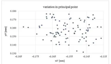
Table 3 shows deviations in the principal distance and principal point up to 20 µm for this specific calibration. It has to be considered that the instability of the camera and its components do not take a similar effect as it would be within a UAV flight. The extend of the variation in principal distance and principal point can be estimated by using the calibration over the VDI testfield since many images are taken from different viewing directions in a larger spatial volume. The resulting variation for the Olympus camera results to a range of 44 µm for the principal distance (Figure 4) and 45 µm for the principal point components (Figure 5).
Figure 4. Variation in principal distance for Olympus camera The International Archives of the Photogrammetry, Remote Sensing and Spatial Information Sciences, Volume XL-1/W4, 2015
Figure 5. Variation in principal point for Olympus camera
3.4 Impact in object space
In order to evaluate the impact of the different calibration results in object space a test is modelled after a prospecting flight scenario. A testfield at a planar wall (Figure 6) is captured by a set of overlapping images in row. For all signalized points
a. their coordinates in object space, estimated within a bundle adjustment, are transformed to their control point coordinates
b. their within a bundle adjustment estimated coordinates in object space, including pre-calibrated interior orientation parameters, are transformed to their control point coordinates
c. forward intersections for object coordinates are calculated, based on previously estimated interior and exterior orientation parameters using the overlapping images (as it would be in flight, too), and transformed to their control point coordinates
d. forward intersections for object coordinates are calculated, based on previously estimated exterior orientation parameters using the overlapping images and pre-calibrated interior orientation parameters, and transformed to their control point coordinates.
Figure 6. Wall testfield
The results in object space are listed in Table 4. Three camera settings are chosen in order to demonstrate a possible effect of changing settings on the results in object space. The images are taken with a ground sample distance of about 0.2 mm according to the lab test. As expected the b and d scenario, introducing pre-calibrated interior orientation parameters, offer a significant higher accuracy level in object space. As expected, the impact right after calibration or considering coordinates of the bundle adjustment itself show best results. The change of camera settings therefore cause a loss in accuracy, for this test scenario, of about 1 – 2 mm, relatively about 200% up to 640%. This range illustrates the unknown dependency of the settings of calibration to those of image acquisition for object reconstruction. Nevertheless, the introduction of (any) reliable
parameter estimation in a project using comparable camera settings lead to an increasing accuracy level in object space.
standard deviations [mm] in transformation
with respect to control points a b c d
Olympus right after calibration 2.15 0.24 3.76 0.98
Olympus changed to AF-mode (same
distance to test object) 4.17 1.56 11.12 2.49
Olympus changed to MF-mode (no focus) 4.54 1.10 7.87 2.65
Table 4. Impact of calibration estimation in object space
4. FLIGHT SIMULATION
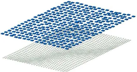
In order to evaluate the impact of the interior orientation parameters on the reconstruction in object space, some UAV flight simulations are used. For this purpose an area of 236 m x 134 m, as it represents a real-world benchmark area, is chosen. Due to nowadays used UAV software packages including dense matching algorithms, an usual image overlap of 80% each along and across the flight direction is used. Figure 7 shows a resulting flight scheme for a flying height of 50 m . The simulation is based on an idealised surface of a double-sinus waveform. This is undulated by 10 m and 30 m respectively. Figure 8 and Figure 9 show a three-dimensional view on the UAV flight scenarios.
Figure 7. Overview on simulated flight order with 80/80 image overlap
Figure 8. Simulated UAV flight scenario above area with 30 m undulation in Z-direction and a flying height of 50 m
Figure 9. Simulated UAV flight scenario above area with 10 m undulation in Z-direction and a flying height of 50 m
The simulation is based on a standard uncertainty for image measurements of 0.003 mm which is equivalent to a bit less than a pixel for the Olympus camera. With respect to the analyses of interior orientation and its estimation within a UAV flight scenario, three types of flight configurations are applied:
1. The first scenario corresponds to a typical flight where all images are taken in the same relative orientation.
2. The second configuration includes additional images taken above the centre of the area by rotating the camera, respectively consecutively changing the yaw angle of the UAV by +90° (see Figure 10).
3. In the third scenario two tilted images are added to the previous configurations by changing the roll angle to 25° and -25° for two images above the centre of the area (see Figure 10).
Figure 10. Additional images for UAV-flight configurations 1 to 3 (numbers in camera symbols indicate scenario)
The processing of the flight simulations follows a usual setup for the bundle adjustment in UAV-photogrammetry. In this case six homogeneous distributed control points are introduced to define the datum. Their standard deviations are set to values of 15 mm for X- and Y- and 30 mm for Z- coordinates. This follows expectable accuracies gained with GPS measurements.
deviation to input
deviation to input
deviation to input
deviation to input
Ck -14.5203 0.0097 -0.0009 -14.5177 0.0090 0.0017 -14.5349 0.0194 -0.0155 -14.5291 0.0183 -0.0097 Xh -0.3530 0.0060 0.0019 -0.3530 0.0050 0.0019 -0.3515 0.0056 0.0034 -0.3537 0.0037 0.0012 Yh 0.1539 0.0060 -0.0050 0.1549 0.0056 -0.0040 0.1566 0.0059 -0.0024 0.1579 0.0042 -0.0010
A1 -2.99E-04 1.84E-06 1.09E-07 -2.98E-04 2.03E-06 1.36E-06
A2 5.32E-07 2.93E-08 3.58E-09 5.18E-07 2.36E-08 -1.01E-08
A3 2.70E-09 1.60E-10 1.60E-11 2.78E-09 1.31E-10 9.68E-11
B1 -3.70E-04 5.18E-06 -5.94E-06 -3.65E-04 5.93E-06 -1.15E-06
B2 2.12E-04 4.60E-06 -4.51E-07 2.13E-04 5.88E-06 2.68E-07
RM Sx 56.5647 54.0502 51.9441 49.0817
RM Sy 56.9475 54.4882 51.9895 49.1083
RM Sz 130.4288 126.6614 123.0858 116.5126
s0 0.0301 0.0301 0.0299 0.0299
RM S(x,y,z) 16.2360 17.2525 18.7632 6.2703 6.0297 12.7277 8.2110 7.3885 33.7752 8.1322 8.5175 9.8338 min -50.7156 -60.9439 -74.6600 -29.1049 -23.3962 -43.7445 -27.9865 -45.3175 -74.3811 -30.8542 -25.3168 -30.4478 max 31.7128 55.6351 38.3410 23.6001 19.5575 43.2544 20.8672 21.1803 48.8647 16.0484 16.8104 18.2000 range 82.4284 116.5790 113.0010 52.7050 42.9537 86.9989 48.8537 66.4978 123.2458 46.9026 42.1272 48.6478
scenario 1: 30m dom undulation, h = 50m scenario 1: 10m dom undulation, h = 50m
result result
Bu
ndl
e a
dj
us
tm
ent
[mm]
int
ers
ec
ti
on
result result
deviation to input
deviation to input
deviation to input
deviation to input
Ck -14.5198 0.0018 -0.0004 -14.5221 0.0016 -0.0027 -14.5093 0.0049 0.0101 -14.5094 0.0048 0.0100 Xh -0.3475 0.0030 0.0074 -0.3504 0.0020 0.0045 -0.3581 0.0036 -0.0032 -0.3577 0.0022 -0.0028 Yh 0.1584 0.0023 -0.0005 0.1594 0.0020 0.0005 0.1599 0.0034 0.0010 0.1600 0.0025 0.0011 A1 -3.01E-04 1.58E-06 -1.24E-06 -3.03E-04 1.44E-06 -3.64E-06
A2 5.47E-07 2.86E-08 1.92E-08 5.97E-07 2.28E-08 6.86E-08
A3 2.58E-09 1.55E-10 -1.02E-10 2.29E-09 1.25E-10 -3.98E-10
B1 -3.61E-04 2.03E-06 3.30E-06 -3.63E-04 3.18E-06 1.14E-06
B2 2.12E-04 1.69E-06 -1.10E-06 2.12E-04 2.92E-06 -4.96E-07
RM Sx 50.1945 49.9646 49.7342 48.9865
RM Sy 50.3886 50.1809 49.7862 49.0128
RM Sz 117.0060 116.9018 117.8215 116.2943
s0 0.0300 0.0300 0.0299 0.0299
RM S(x,y,z) 11.1714 10.7151 14.1030 11.6333 11.0770 16.4061 3.7852 3.3182 13.0357 3.6320 3.3918 8.5650 min -42.0538 -35.8189 -62.1377 -42.8574 -36.9618 -83.7740 -10.5780 -11.5126 -22.3239 -11.0629 -8.9493 -20.0731 max 39.7442 40.1605 46.4178 33.2964 37.6425 39.9380 8.7748 8.3916 40.8271 6.4956 7.3357 27.5132 range 81.7980 75.9794 108.5555 76.1538 74.6043 123.7120 19.3528 19.9042 63.1510 17.5585 16.2850 47.5863
scenario 3: 30m dom undulation, h = 50m scenario 3: 10m dom undulation, h = 50m
int
ers
ec
ti
on
result result
Bu
ndl
e a
dj
us
tm
ent
result result
[mm]
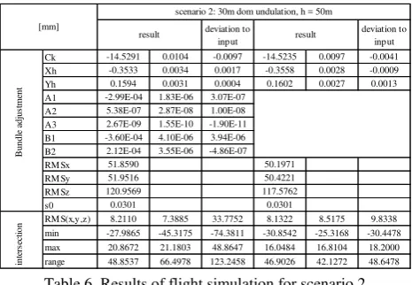
Table 5. Results of flight simulation for scenario 1 and 3
deviation to input
deviation to input Ck -14.5291 0.0104 -0.0097 -14.5235 0.0097 -0.0041 Xh -0.3533 0.0034 0.0017 -0.3558 0.0028 -0.0009 Yh 0.1594 0.0031 0.0004 0.1602 0.0027 0.0013 A1 -2.99E-04 1.83E-06 3.07E-07
A2 5.38E-07 2.87E-08 1.00E-08 A3 2.67E-09 1.55E-10 -1.90E-11 B1 -3.60E-04 4.10E-06 3.94E-06 B2 2.12E-04 3.55E-06 -4.86E-07
RM Sx 51.8590 50.1971
RM Sy 51.9516 50.4221
RM Sz 120.9569 117.5762
s0 0.0301 0.0301
RM S(x,y,z) 8.2110 7.3885 33.7752 8.1322 8.5175 9.8338 min -27.9865 -45.3175 -74.3811 -30.8542 -25.3168 -30.4478 max 20.8672 21.1803 48.8647 16.0484 16.8104 18.2000 range 48.8537 66.4978 123.2458 46.9026 42.1272 48.6478
result
Bu
ndl
e a
dj
us
tm
ent
int
ers
ec
ti
on
[mm]
result
scenario 2: 30m dom undulation, h = 50m
Table 6. Results of flight simulation for scenario 2 Table 5 and Table 6 summarize the results of the described investigations based on flight simulations. The analyses are done by 1) adjusting all interior orientation parameters and 2) adjusting only the principal distance and principal point by introducing pre-calibrated distortion parameters.
For each result the adjusted parameters of interior orientation and its standard deviations are collected. The RMS-values of all object points as well as the s0 value (standard deviation of unit weight) estimate the statistical precision level of the simulated data set. In order to evaluate the impact of the systems’ configuration, forward intersections are calculated for a set of 60 object points. Afterwards these coordinates are transformed to a set of control point coordinates. The remaining deviations are summarized as RMS-values in X, Y and Z. In addition the minimum and maximum values as well as the subsequent range of deviations are summarized. The results of forward intersection can be taken as absolute accuracy level for these investigations and indicate the impact of different scenarios in object space.
The results show an increase in the object space accuracy for X- and Y-direction by introducing yaw-changed images (scenario 2) in contrast to a standard data set (scenario 1). If tilted images are introduced the accuracy for the Z-direction rises, too (scenario 3). An increase in Z-direction accuracy is also possible considering pre-calibrated distortion parameters. In all cases the overall accuracy in object space is increasing (RMS-values and range) compared to the almost stable statistical precisions in the RMS-values from the bundle adjustment.
Considering an instable principal distance and principal point to the flight scenario, the results in object space decrease as expected. Expecting a statistical variation of these three components of 0.01 mm, the remaining accuracies in object space decrease about 120% to 400% (see Table 7). The percentage decrease is less with scenario 3 where rolled images have been introduced.
scenario 1: 30m dom undulation, h = 50m 224.0198 191.3321 406.9649 scenario 3: 30m dom undulation, h = 50m 120.6109 118.2818 181.2093 scenario 3: 10m dom undulation, h = 50m 192.1743 210.7108 174.2395 decrease in object space accuracy when considering instable principal distance and
principal point [%]
Table 7. Percentage decrease in object space accuracy considering instable interior orientation
A higher undulation of the surface lead to a more significant and reliable estimation of the interior orientation parameters.
This is especially obvious and to be expected for the principal distance. Its reliability increases when using scenario 3 and should be considered as requirement for a flight scenario if self-calibration is utilized.
It can be observed that the simulations with a less undulating surface lead to a higher accuracy level in object space. This effect can also be observed when using a larger flying height, e.g. with 75 m.
In general the bundle adjustment results shown in Table 5 and Table 6 have to be considered as statistical data, especially when evaluating the interior orientation parameters. The generated forward intersections and the subsequent derived accuracies in object space demonstrate the dependency on the whole bundle system. While very small deviations to the input data are remaining, the standard deviations of the interior orientation parameters are still high within several microns. This also leads to an influence to the whole system and therefore causes higher deviations in object space. Only when introducing additional, tilted images to the bundle, the standard deviations of the interior orientation parameters are increasing and lead to an increase in object space accuracy.
The resulting accuracies in object space are still influenced by the camera and its interior orientation. Object space accuracies in the order of several ground pixels (GSD) show the limits in standard UAV scenarios. The investigations on image blocks that allow for adequate self-calibration to not replace a metric UAV camera and a serious calibration. However, they help for awareness of additional influences on the accuracy in object space.
5. SUMMARY
Within these investigations on the impact of the interior orientation parameters in object space different aspects are analysed further. On the one hand nowadays used consumer cameras in UAV photogrammetry, e.g. an Olympus Pen E-PM2 or other system cameras, are analysed with respect to their internal stability and reliability of the chosen parameter set. In addition, the influence of the camera calibration procedure itself is estimated. On the other hand simulation based UAV flight analyses are evaluated in order to investigate adequate flight scenarios for self-calibration.
The camera calibration procedures of Agisoft Lens and OpenCV are compared with respect to a photogrammetric approach. For the results of an Olympus Pen E-PM2 camera it can be summarized that using a strong image block configuration on a planar chessboard pattern, as it is used in computer vision applications, relatively reliable parameters are estimated. For the Olympus Pen E-PM2 camera itself, a high correlation between the components of the principal point and the decentring distortion can be observed. This is not only true for the statistical correlation but also for the resulting parameters itself. They result to significantly different values depending on the set of estimated parameters for the interior orientation. With respect to the camera calibration, these parameters should not be removed as they lead to an under-parametrization of the system and therefore to erroneous results for the remaining parameter.
This is probably caused by an instability of the camera components. The camera is based on an auto-focus lens, as many consumer cameras do. In addition, a variation of the The International Archives of the Photogrammetry, Remote Sensing and Spatial Information Sciences, Volume XL-1/W4, 2015
principal distance and the principal point, estimated for each image separately, is visible.
The investigations on flight scenarios allowing for adequate self-calibration show the necessity of introducing rolled images to a UAV flight scenario. In order to allow for stable and accurate object coordinates in all three coordinate directions, these additional images are recommended. Furthermore, this leads to a higher level of significance for the interior orientation parameter estimation. The camera instability, that should be expected when using consumer cameras, causes a loss in accuracy of at least 200%. The results in object space show the limit of standard UAV scenarios as the remaining deviations in object space are up to the extend of several ground pixels. If self-calibration is used with UAV flights one should be aware of the quality and significance of the parameter estimation. A pre-calibration should be introduced if possible.
REFERENCES
Brown, D. C. (1971): Close-Range Camera Calibration. Photogrammetric Engineering, Vol. 37, Nr. 8, S. 855-866
Colomina, I., Molina, P. (2014): Unmanned aerial systems for photogrammetry and remote sensing: A review. ISPRS Journal of Photogrammetry and Remote Sensing, 92 (2014), S. 79-97
Cramer, M., Haala, N., Gültlinger, M., Hummel, R. (2014):
RPAS im operationellen Einsatz beim LGL Baden-Württemberg – 3D-Dokumentation von Hangrutschungen. Publikationen der DGPF Nr. 23
Douterloigne, K., Gautama, S., Philips, W. (2009): Fully automatic and robust UAV camera calibration using chessboard patterns. IEEE IGARSS 2009, S. II-551-554
Hastedt, H. (2015): Entwicklung einer Simulation zur Genauigkeitsevaluation der Kamerakalibrierung mit OpenCV. Master Thesis.
Heikkila, J., Silvén, O. (1997): A Four-step Camera Calibration Procedure with Implicit Image Correction. Proceedings of IEEE Society Conference on Computer Vision and Pattern Recognition, S. 1106-1112
Kruck, E., Mélykuti, B. (2014): Kalibrierung von Oblique und UAV Kameras. Publikationen der DGPF Nr. 23
Luhmann, T., Robson, S., Kyle, S., Boehm, J. (2014): Close-Range Photogrammetry and 3D Imaging. De Gruyter textbook, 2nd edition, ISBN 978-3-11-030269-1
Pérez, M., Agüera, F., Carvajal, F. (2011): Digital camera calibration using images taken from an unmanned aerial vehicle. International Archives of Photogrammetry, Remote Sensing and Spatial Information Sciences, Vol. XXXVIII-1/C22, UAV-g 2011
Remondino, F., Fraser, C.S. (2006): Digital camera calibration methods: considerations and comparisons. The International Archives of Photogrammetry, Remote Sensing and Spatial Information Sciences, Vol. 36(5), S. 266-272
VDI (2002): Optische 3D-Messsysteme, Bildgebende Systeme mit punktförmiger Antastung. Verein Deutscher Ingenieure – Verband der Elektrotechnik, Elektronik Informationstechnik VDI/VDE, 2634 Blatt 1 (German guideline on optical 3D
measuring systems – Imaging systems with point-by-point probing)
Zhang, Z. (2000): A flexible new technique for camera calibration. Microsoft Research, Technical Report MSR-TR-98-71