Analytical solutions for solute transport in
saturated porous media with semi-infinite or
finite thickness
Youn Sim & Constantinos V. Chrysikopoulos*
Department of Civil and Environmental Engineering, University of California, Irvine, CA 92697, USA
(Received 5 April 1997; revised 19 June 1998; accepted 25 June 1998)
Three-dimensional analytical solutions for solute transport in saturated, homogeneous porous media are developed. The models account for three-dimensional dispersion in a uniform flow field, first-order decay of aqueous phase and sorbed solutes with different decay rates, and nonequilibrium solute sorption onto the solid matrix of the porous formation. The governing solute transport equations are solved analytically by employing Laplace, Fourier and finite Fourier cosine transform techniques. Porous media with either semi-infinite or finite thickness are considered. Furthermore, continuous as well as periodic source loadings from either a point or an elliptic source geometry are examined. The effect of aquifer boundary conditions as well as the source geometry on solute transport in subsurface porous formations is investigated. q1999 Elsevier Science Ltd. All rights reserved.
Keywords: solute transport, analytical solution, multidimensional systems, nonequili-brium sorption, first-order decay.
NOMENCLATURE
a semi-axis of the elliptic source parallel to the x-axis [L]
a1, a2 defined in eqns (22) and (23), respectively
A defined in eqn (5)
b semi-axis of the elliptic source parallel to the y-axis [L]
B defined in eqn (6)
C solute concentration in suspension (liquid
phase) [M L¹3]
C0 source concentration [M L¹3]
C* sorbed solute concentration (solute mass/solids mass) [M M¹1]
C` steady-state solute concentration in the absence of decay [M L¹3]
Dx longitudinal hydrodynamic dispersion
coeffi-cient [L2t¹1]
Dy lateral hydrodynamic dispersion coefficient [L2t¹1]
Dz vertical hydrodynamic dispersion coefficient
[L2t¹1]
erf[x] error function, equal to(2=p1=2)
Zx
0e ¹z2dz
E defined in eqn (B2)
E defined in eqn (A2)
f, f0, f1, f2 arbitrary functions
F general functional form of virus source config-uration [M L¹3t¹1]
Printed in Great Britain. All rights reserved 0309-1708/99/$ - see front matter
PII: S 0 3 0 9 - 1 7 0 8 ( 9 8 ) 0 0 0 2 7 - X
507
F¹1 Fourier inverse operator
Ffc finite Fourier cosine transform operator
Ffc¹1 finite Fourier cosine inverse operator
g defined in eqn (B9)
G source loading function [M t¹1(point source); M L¹2t¹1(elliptic source)]
H finite aquifer thickness [L]
H defined in eqn (7)
I0[·] modified Bessel function of first kind of order zero
I1[·] modified Bessel function of first kind of first
order
K0[·] modified Bessel function of second kind of
order zero
lx0,ly0,lz0 x, y and z Cartesian coordinates, respectively, of a point source or the center of an elliptic source [L]
L¹1 Laplace inverse operator
m integer summation index
p dummy integration variable
P defined in eqn (A27)
q dummy integration variable
Q defined in eqn (A17)
r radius of circular source [L]
r1 forward rate coefficient [t¹1]
r2 reverse rate coefficient [t¹1]
s Laplace transform variable with respect to time
S defined in eqn (B7)
t time [t]
U average interstitial velocity [L t¹1]
v dummy integration variable
W source geometry function [L¹3]
x,y,z spatial coordinates [L]
Greek symbols .
a arbitrary constant
ax longitudinal dispersivity [L]
ay lateral dispersivity [L]
az vertical dispersivity [L]
b,b1,b2 arbitrary constants
g Fourier transform variable with respect to
spatial coordinate x
d(·) Dirac delta function
z dummy integration variable
h defined in eqn (A23)
v porosity (liquid volume/porous medium
volume) [L3L¹3]
k,k1,k2 defined in eqns (26a), (24) and (25), respectively
l decay rate of liquid phase solute [t¹1
]
l* decay rate of sorbed solute [t¹1]
L1,…,L6 defined in eqns (17a)–(17d), (21) and (30),
respectively
y dummy integration variable
r bulk density of the solid matrix (solids mass/
aquifer volume) [M L¹3]
t dummy integration variable
f Laplace transform variable with respect to
spatial coordinate z
F defined in eqn (A8)
wm finite Fourier cosine transform variable with
respect to spatial coordinate z, defined in eqn (31)
W defined in eqn (B6)
q Fourier transform variable with respect to
spatial coordinate y
1 INTRODUCTION
and fate of contaminants in the subsurface. For well-defined, ideal aquifers, analytical solute transport models are frequently employed. Furthermore, analytical models are often used for verifying the accuracy of numerical solutions to complex solute transport models.
Multidimensional contaminant transport models have several advantages over one-dimensional models. For exam-ple, multidimensional models can account for concentration gradients and contaminant transport in directions perpendicu-lar to the groundwater flow. As indicated by Leij and Dane,14 measuring experimentally lateral and vertical dispersion coef-ficients is not a trivial task. However, multidimensional trans-port models can provide such parameters by direct fitting of available experimental data. In addition, multidimensional models can easily account for a variety of boundary condi-tions, as well as contaminant source geometries.
Although several multidimensional analytical models for solute or colloid/virus transport are available in the litera-ture,1,3–5,8,10,14,15,20,22,23 multidimensional analytical models that can accommodate a variety of contamination source configurations in porous media with semi-infinite or finite thickness are nonexistent.
The present study extends the collection of contaminant transport models by presenting analytical solutions to multi-dimensional transport through saturated, homogeneous por-ous media, accounting for first-order decay of the solute in the aqueous phase or sorbed onto the solid matrix with different decay rates. A variety of source configurations, including continuous as well as periodic source loadings from either point or elliptic source geometries, are consid-ered. Generalized analytical solutions applicable to solute as well as virus transport in aquifers of semi-infinite and finite thickness are derived.
2 MODEL DEVELOPMENT
The transport of solutes in saturated, homogeneous porous media, accounting for three-dimensional hydrodynamic dis-persion in a uniform flow field, nonequilibrium sorption, and first-order decay of liquid phase and sorbed solutes with different decay rates, is governed by the following partial differential equation:
]C(t,x,y,z)
where C is the liquid phase solute concentration; C* is the solute concentration sorbed onto the solid matrix; Dx, Dy and Dz are the longitudinal, lateral and vertical hydrody-namic dispersion coefficients, respectively; U is the average
interstitial velocity; t is time; x, y and z are the spatial coor-dinates in the longitudinal, lateral and vertical directions, respectively; r is the bulk density of the solid matrix; vis the porosity of the porous medium; l is the decay rate of liquid phase solutes; l* is the decay rate of sorbed solutes; and F is a general form of the source configuration. It should be noted that the effective porosity, defined as percentage of interconnected pore space, may be employed instead of por-osity in a porous medium that contains a large number of dead-end pores or in a fractured porous formation.2,7
The accumulation of solutes onto the solid matrix is described by the following nonequilibrium expression:
r
where r1and r2are the forward and reverse rate coefficients.
Assuming that initially there are no sorbed solutes present in the porous formation, the expression describing C* is obtained by solving eqn (2) subject to the initial condition
C*(0,x,y,z)¼0 to yield
wheretis a dummy integration variable. In view of eqns (2) and (3), the governing equation, eqn (1), can be written as
where the following substitutions have been employed
A¼r1þl, (5)
B¼r1r2, (6)
H¼r2þlp: (7)
The derived integrodifferential equation, eqn (4), is solved analytically in the subsequent sections for the cases of aquifers with semi-infinite and finite thickness.
2.1 Source configuration
The source configuration is represented by the following general function:
F(t,x,y,z)¼G(t)W(x,y,z), (8)
area and W(x,y,z) characterizes the source physical geome-try. In this work, point as well as two-dimensional source geometries are considered. Furthermore, G(t) characterizes the source loading type. Although instantaneous or contin-uous/temporally periodic source loading types can easily be employed, the present research efforts focus only on a con-tinuous/temporally periodic source loading.
2.1.1 Point source geometry
The point source geometry is described mathematically by the following expression:
W(x,y,z)¼1
vd(x¹lx0)d(y¹ly0)d(z¹lz0), (9) where lx0,ly0,lz0 represent the x,y,z unbounded
(¹` ,lx0,ly0,lz0, `) Cartesian coordinates of the point source, respectively, and d is the Dirac delta function. It should be noted that here G represents the solute mass release from the point source.
2.1.2 Elliptic source geometry
The elliptic source geometry is described mathematically by the following expression:
W(x,y,z)¼
d(z¹lz0)
v
(x¹lx0)
2
a2 þ
(y¹ly0)
2
b2 #1,
0 otherwise,
8 > <
> :
(10)
where lx0,ly0,lz0 are x,y,z Cartesian coordinates, respec-tively, of the center of the elliptic source geometry, and a and b represent the semi-axes of the ellipse parallel to the x-and y-axes, respectively. It should be noted that here G signifies the solute mass release rate per unit source area.
2.2 Aquifer with semi-infinite thickness
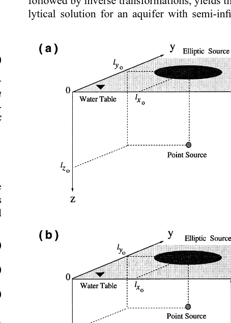
The appropriate initial and boundary conditions for the case of an aquifer with infinite longitudinal and lateral directions and semi-infinite vertical direction (thickness), as illustrated schematically in Fig. 1(a), are as follows:
C(0,x,y,z)¼0, (11)
C(t,6 `,y,z)¼0, (12)
C(t,x,6 `,z)¼0, (13)
]C(t,x,y,0)
]z ¼0, (14)
]C(t,x,y,`)
]z ¼0, (15)
where condition (11) corresponds to the situation in which solutes are initially absent from the three-dimensional por-ous formation, eqns (12) and (13) indicate that the aquifer is infinite horizontally and laterally, boundary condition (14) represents a zero dispersive flux boundary and eqn
(15) preserves concentration continuity for a semi-infinite vertical aquifer thickness. The vertical level z¼0 defines the location of the water table or a confining layer. Eqn (4), subject to conditions (11)–(15), is solved analytically. It should be noted that z increases in the downward direction. The analytical solution to the governing partial differen-tial equation, eqn (4), can be derived by a variety of meth-ods, including the conventional method of separation of variables, as well as integral transform methods. Further-more, a solution technique developed by Walker24 invol-ving a Green function (fundamental solution) can also be utilized. However, in the present study, integral transform techniques were employed because the multidimensional models developed are an extension of our previous analy-tical work on virus transport models,19,20 where Laplace transform techniques were employed. Similar mathematical techniques were employed for the analytical solutions of multidimensional solute transport by Toride et al.21 and Shan and Javandel.18
Taking Laplace transforms with respect to time variable t and space variable z, and Fourier transforms with respect to space variables x and y of eqn (4), and subsequently employ-ing the transformed initial and boundary conditions, followed by inverse transformations, yields the desired ana-lytical solution for an aquifer with semi-infinite thickness
Fig. 1. Schematic illustration of point and elliptic sources of
con-tamination with coordinates lx0,ly0,lz0 in an aquifer with semi-infinite (a) and finite (b) thickness. Note that the positive direction
(see Appendix A):
where p, q, v andz are dummy integration variables; the following definitions were employed:
L1(t)¼exp½¹Htÿ, (17a)
and I1 is the modified Bessel function of the first kind of
first order.
2.2.1 Point source geometry
Substituting eqns (8) and (9) into eqn (16) yields the analy-tical solution for the case of point source geometry:
C(t,x,y,z)¼ 1
where L1–L4 are defined in eqns (17a)– (17d), respec-tively, and the following property of the Dirac delta func-tion was employed:
Zb
af0(t)d(t¹t0)dt¼f0(t0), a#t0#b, (19) whereaandbare arbitrary constants, and f0is an arbitrary
function.
2.2.2 Elliptic source geometry
Substituting eqns (8) and (10) into eqn (16) leads to the analytical solution for the case of elliptic source geometry:
C(t,x,y,z)¼ 1
whereL1–L4are defined in eqns (17a)– (17d), respectively,
L5(t)¼erfk1(t,q,y)
erf[·] is the error function, and the following transformation and integral relationships were employed:
k¼ y¹v
As noted by Chrysikopoulos,4solving for an elliptic source geometry is advantageous because the appropriate solution for a circular source can easily be obtained by setting a¼b ¼r in eqns (22)–(25), where r is the radius of the circular
source.
2.3 Aquifer with finite thickness
The desired analytical solution for the case of an aquifer with finite thickness, as illustrated schematically in Fig. 1(b), is obtained by solving eqn (4) subject to conditions (11)–(14) and the following finite vertical, lower boundary condition:
]C(t,x,y,H)
]z ¼0, (28)
(28) implies that the aquifer is confined by an impermeable layer at depth z¼ H. Taking the Laplace transform with
respect to the time variable t, Fourier transforms with respect to space variables x and y, and the finite Fourier cosine transform with respect to the space variable z of eqn (4), and subsequently employing the transformed initial and boundary conditions, followed by inverse transformations yields (see Appendix B):
C(t,x,y,z)¼ 1
whereL1–L3are defined in eqns (17a)–(17c), respectively,
L6(t,f1,f2)¼ f1
m is the integer summation index,F(t,¨ x,y,wm) represents the finite Fourier cosine transform of F(t,x,y,z) with respect to space variable z with corresponding finite Fourier cosine transform variablewm, and f1and f2are arbitrary functions.
2.3.1 Point source geometry
The desired analytical solution for the case of point source geometry is obtained by substituting the corresponding expression forF(t,¨ x,y,wm)into eqn (29). Substituting eqn (9) into eqn (8) and subsequently taking the finite Fourier cosine transform (defined in eqn (B3)) with respect to space variable z of the resulting expression yields
¨
where the latter formulation in eqn (32) is a consequence of employing eqn (19). In view of eqns (19) and (32), the general solution, eqn (29), reduces to the following form:
C(t,x,y,z)¼ 1
2.3.2 Elliptic source geometry
In view of eqn (10), the finite Fourier cosine transform of eqn (8) with respect to z is given by
¨
0 otherwise:
8
Substituting eqn (34) into eqn (29), the desired analytical solution for the case of elliptic source geometry is as follows: (17c), (21) and (30), respectively.
3 MODEL SIMULATIONS AND DISCUSSION
Model simulations are performed for two different source configurations, and aquifers with either semi-infinite or finite thickness. The integrals present in the analytical solu-tions (18), (20), (33) and (35) are evaluated numerically by the integration routines Q1DA and QDAG, which utilize globally adaptive quadrature algorithms.11,12 The infinite series part of the solution for the case of an aquifer with finite thickness (eqn (30)) is evaluated by considering up to 1000 terms (m¼1000). The number of terms, m, is selected so that additional terms do not alter the summation more than 0.001%.
The groundwater table and the bottom of the finite thick-ness aquifer are assumed to be located at z¼0 cm and z¼H ¼ 100 cm, respectively. Although all analytical solutions derived here are general enough to account for temporally
Table 1. Model parameters for simulations
Parameter Value Reference
Fig. 2. Comparison between the analytical solution derived in this work for a point source geometry with constant mass release rate (solid
curve) and the corresponding solution of the one-dimensional model presented by Sim and Chrysikopoulos19(circles). Here, D
y¼Dz. 0 cm2h¹1, lx0¼200 cm, ly0¼0 cm, lz0¼50 cm, r1¼ 0.03 h
¹1
, r2¼0.017 h ¹1
, t¼1 day, y¼0:1cm and z¼50 cm.
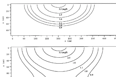
Fig. 3. Concentration contours in the x–z plane obtained for a point source within an aquifer of semi-infinite thickness at t¼50 days (a), t ¼100 days (b) and t¼300 days (c). Here, lx0¼200 cm, ly0¼0 cm, lz0¼50 cm, r1¼0.1 h
¹1
, r2¼0.0008 h ¹1
periodic source loading, for simplicity, the model simula-tions presented are based on a constant solute mass release rate and the value of G is set to unity. Unless otherwise specified, the fixed parameter values used in the simulations are those listed in Table 1.
For the case where Dy¼Dz.0 cm2h¹1, the analytical
solution derived in this work for a point source geometry with constant solute mass release rate is equivalent to the one-dimensional analytical solution for virus transport with constant concentration boundary conditions presented by Sim and Chrysikopoulos19 (eqn (31)). For this special case, model simulations are compared in Fig. 2 against the one-dimensional model derived by Sim and Chrysikopou-los.19 It should be noted, however, that in Fig. 2 the con-centrations simulated by the one-dimensional transport model (circles) are normalized with the source concentra-tion (C0), whereas concentrations generated by solutions
derived in this work (solid curves) are normalized with the steady-state concentration (C`) evaluated at t ¼
400 days, as suggested by Hunt.10 Fig. 2 clearly indicates
that the model simulations compared are virtually identical.
Fig. 3 illustrates two-dimensional snapshots of solute concentration at three successive times simulated for an aquifer with semi-infinite thickness (eqn (18)). A point source is assumed to be located inside the aquifer at
lx
0¼200 cm, ly0¼0 cm and lz0¼50 cm. It is observed that as the solute plume spreads with increasing time, solute spreading is restricted at the groundwater table (z¼
0 cm), with a consequent zero gradient of solute concentra-tion distribuconcentra-tion, whereas a continuous solute spreading occurs anywhere else below the water table because the aquifer extends to infinity without a boundary (eqn (15)). Consequently, the observed solute plume is asymmetric with respect to the flow direction along the plume center-line. In contrast, Fig. 4 illustrates symmetric solute plumes at three successive times, for an aquifer with finite thickness and point source geometry (eqn (33)). This is due to the presence of a fixed impermeable lower boundary (eqn (28), z¼H¼100 cm) in addition to the upper groundwater Fig. 4. Concentration contours in the x–z plane obtained for a point source within an aquifer of finite thickness at t¼ 50 days (a), t¼
100 days (b) and t¼300 days (c). Here, lx0¼200 cm, ly0¼0 cm, lz0¼50 cm, r1¼0.03 h
¹1
table boundary (z¼0 cm). Comparing Figs 3 and 4, it is clear that the vertical migration of solutes is hindered by the two fixed boundaries. Furthermore, the presence of these boundaries contributes to the enhancement of solute trans-port downstream from the source in the direction of ground-water flow.
The effect of the lower impermeable boundary condition is also demonstrated for the case of an elliptic source geometry. Two-dimensional snapshots of solute concentrations at t ¼
300 days are predicted for the case of an elliptic source geometry for an aquifer with semi-infinite thickness (eqn (20), Fig. 5(a)), as well as for an aquifer with finite thickness (eqn (35), Fig. 5(b)). Similarly to the case of point source geometry, the presence of a shallow impermeable aquitard significantly constricts the vertical spreading of solutes, which consequently leads to an enhanced solute migration in the direction of groundwater flow.
The analytical solutions derived in this work can be read-ily employed to simulate transport of a variety of contami-nants, including biocolloids such as viruses and bacteria. The applicability of these models to field investigations is limited to subsurface formations, where it may not be pos-sible to account for physicochemically heterogeneous
por-ous media. However, it should be noted that
multidimensional contaminant transport models are more advantageous than one-dimensional models where a homo-geneous porous medium assumption is valid, because they can account for concentration gradients and contaminant transport in directions perpendicular to the groundwater flow. Furthermore, multidimensional models can easily
account for a variety of boundary conditions, as well as contaminant source geometries.
4 SUMMARY
Three-dimensional analytical solutions for solute transport in saturated, homogeneous porous media were developed, accounting for three-dimensional hydrodynamic disper-sion in a uniform flow field, first-order decay of aqueous phase and sorbed solutes with different decay rates, and nonequilibrium solute sorption onto the solid matrix of the porous formation. The governing transport equations were solved analytically by employing Laplace, Fourier and finite Fourier cosine transform techniques. Aquifers with either semi-infinite or finite thickness are considered. The derived analytical solutions are general enough to accom-modate a variety of source loadings and source geome-tries. However, the simulations presented in this study are based on a continuous source loading from either point source or elliptic source geometry. It was shown that solute transport in subsurface porous media is signifi-cantly influenced by the aquifer boundary conditions. For an aquifer confined by a shallow impermeable aquitard, solute migration in the vertical direction is restricted, whereas solute transport in the direction of groundwater flow is enhanced, compared with the case of a relatively thick aquifer. The analytical solutions developed here are particularly useful for preliminary estimation of solute migration, characterization of Fig. 5. Concentration contours in the x–z plane obtained for an elliptic source geometry, and an aquifer with semi-infinite (a) and finite (b)
thickness. Here, a¼b¼25 cm, lx0¼200 cm, ly0¼lz0¼0 cm, r1¼0.1 h
¹1
contamination sources, examination of possible aquifer boundary conditions, validation of numerical solutions and determination of solute transport parameters from laboratory or well-defined field experiments.
ACKNOWLEDGEMENTS
This work was sponsored jointly by the National Water Research Institute and the University of California, Water Resources Center, as part of Water Resources Center Pro-ject UCAL-WRC-854. The content of this manuscript does not necessarily reflect the views of the agencies and no official endorsement should be inferred.
REFERENCES
1. Batu, V. A generalized two-dimensional analytical solute transport model in bounded media for flux-type finite multiple sources. Water Resour. Res., 1993, 29(8), 1125– 1132.
2. Bear, J., Dynamics of Fluids in Porous Media. Dover, 1972. 3. Bellin, A., Rinaldo, A., Bosma, W. J. P., van der Zee, S. E. A. T. M. and Rubin, Y. Linear equilibrium adsorbing solute transport in physically and chemically heterogeneous porous formations. 1. Analytical solutions. Water Resour. Res., 1993, 29(12), 4019–4030.
4. Chrysikopoulos, C. V. Three-dimensional analytical models of contaminant transport from nonaqueous phase liquid pool dissolution in saturated subsurface formations. Water Resour. Res., 1995, 31(4), 1137–1145.
5. Chrysikopoulos, C. V., Voudrias, E. A. and Fyrillas, M. M. Modeling of contaminant transport resulting from dissolution of nonaqueous phase liquid pools in saturated porous media. Trans. Porous Media, 1994, 16(2), 125–145.
6. Churchill, R. V., Operational Mathematics. McGraw-Hill, New York, 1958.
7. Domenico, P. A. & Schwartz, F. W., Physical and Chemical Hydrogeology. John Wiley, New York, 1990.
8. Goltz, M. N. and Roberts, P. V. Three-dimensional solutions for solute transport in an infinite medium with mobile and immobile zones. Water Resour. Res., 1986, 22(7), 1139– 1148.
9. Gradshteyn, I. S. & Ryzhik, I. M., Table of Integral, Series, and Products. Academic Press, New York, 1980.
10. Hunt, B. Dispersive sources in uniform groundwater flow. J. Hydraul. Div., Am. Soc. Civ. Engng, 1978, 104(HY1), 75–85. 11. IMSL, IMSL MATH/LIBRARY User’s Manual, version 2.0.
IMSL, Houston, 1991.
12. Kahaner, D., Moler, C. & Nash, S., Numerical Methods and Software. Prentice Hall, Englewood Cliffs, NJ, 1989. 13. Kreyszig, E., Advanced Engineering Mathematics, 7th ed.
John Wiley, New York, 1993.
14. Leij, F. J. and Dane, J. H. Analytical solutions of the one-dimensional advection equation and two- or three-dimensional dispersion equation. Water Resour. Res., 1990,
26(7), 1475–1482.
15. Leij, F. J., Skaggs, T. H. and van Genuchten, M. Th. Analytical solutions for solute transport in three-dimensional semi-infinite porous media. Water Resour. Res., 1991,
27(10), 2719–2733.
16. Park, N., Blanford, T. N. & Huyakorn, P. S., VIRALT: A Modular Semi-analytical and Numerical Model for Simulating Viral Transport in Ground Water. International
Ground Water Modeling Center, Colorado School of Mines, Golden, CO, 1992.
17. Roberts, G. E. & Kaufman, H., Table of Laplace Transforms. W. B. Saunders, Philadelphia, PA, 1966.
18. Shan, C. and Javandel, I. Analytical solutions for solute transport in a vertical aquifer section. J. Contam. Hydrol., 1997, 27(1)2, 63–82.
19. Sim, Y. & Chrysikopoulos, C. V., Analytical models for one-dimensional virus transport in saturated porous media. Water Resour. Res., 31(5) (1995) 1429–1437. [Correction, Water Resour. Res., 32(5), (1996) 1473].
20. Sim, Y. and Chrysikopoulos, C. V. Three-dimensional analytical models for virus transport in saturated porous media. Transport in Porous Media, 1998, 30(1), 87–112. 21. Toride, N., Leij, F. J. and Van Genuchten, M. T. A
comprehensive set of analytical solutions for
nonequilibrium solute transport with 1st-order decay and zero-order production. Water Resour. Res., 1993,
29(7), 2167 – 2182.
22. van Dujin, C. J. and van der Zee, S. E. A. T. M. Solute transport parallel to an interface separating two different porous materials. Water Resour. Res., 1986, 22(13), 1779– 1789.
23. van Kooten, J. J. A. A method to solve the advection– dispersion equation with a kinetic adsorption isotherm. Adv. Water Resour., 1996, 19(4), 193–206.
24. Walker, G. R. Solution to a class of coupled linear partial differential equations. IMA J. Appl. Math., 1987, 38, 35 – 48.
25. Yates, M. V. and Ouyang, Y. VIRTUS, a model of virus transport in unsaturated soils. Appl. Environ. Microb., 1992, 58(5), 1609–1616
APPENDIX A DERIVATION OF THE ANALYTICAL SOLUTION FOR AN AQUIFER WITH SEMI-INFINITE THICKNESS
The analytical solution for the case of semi-infinite thick-ness is obtained by solving eqn (4) subject to conditions (11)–(15). Taking Laplace transforms with respect to time variable t and space variable z, and Fourier transforms with respect to space variables x and y of eqn (4) and subse-quently employing eqn (11) and transformed boundary condition (14) yields
˜
and the following properties were employed for the Laplace and Fourier transformations:13,17
¯ˆ˜
where the tilde and overdot signify Laplace transform with respect to time and space variables t and z, respectively, and s and f are the corresponding Laplace domain vari-ables; the hat and overbar signify Fourier transforms with respect to space variables x and y with corresponding Fourier domain variables g and q, respectively; and
i¼(¹1)1/2.
Taking the Laplace inverse transformation of eqn (A1) with respect to f, applying boundary condition (15) and
subsequently evaluating C(s,¯ˆ˜ g,q,0) at the limit z → `,
and the following Laplace inversion identities were uti-lized:17
whereL¹1is the Laplace inverse operator, andaandbare
arbitrary constants.
Furthermore, for mathematical convenience, let
F¼ HF sþHþ
sF
sþH: (A12)
The inverse Laplace transformation of eqn (A12) with respect to s can be found by employing the following relationship:19
wheref˜0(s)is the Laplace transform of the arbitrary func-tion f0(t) andais an arbitrary constant. Following the
pro-cedures provided in Sim and Chrysikopoulos,19the inverse
Laplace transform of eqn (A12) is obtained as
L¹1 HF(s,g,q,z)
In view of eqns (A12) and (A14), and application of the convolution theorem, the inverse Laplace transformation of eqn (A7) with respect to s is given by
¯ˆ
The inverse Fourier transformation of eqn (A18) with respect to gis
where the following definitions of the Fourier inverse transform were employed:
F¹1fˆ1(g) whereF¹1is the Fourier inverse operator andyis a dummy integration variable.
In order to obtain the inverse Fourier transformation of eqn (A15) with respect tog, only the termQ(g,t) defined in eqn (A17) requires inversion, and is obtained as follows:
F¹1Q(g,t)
and the latter expression in eqn (A22) is a consequence of employing Euler’s formula (eigx¼cos(gx)þisin(gx)) and
the integral identities found in Gradshteyn and Ryzhik9 (eqn 3.923.1 and 2, p. 485) were utilized. Therefore, in view of eqn (A22), the inverse Fourier transformation of eqn (A15) is
The inverse Fourier transformation of eqn (A19) with respect toqis
C(t,x,y,z)¼ 1
In view of the following inverse Fourier transform relation-ship (see Kreryszig,13eqn 9, p. 621):
F¹1 exp ¹q2Dyz
the inverse Fourier transformation of eqn (A24) is
P(t,x,y,z)¼e¹Ht
Furthermore, in order to complete the description of eqn (A25), the derivative of P(t,x,y,z) with respect to t is obtained as follows:
]P(t,x,y,z)
Substituting eqn (A23) into eqns (A27) and (A28) and sub-sequently substituting the resulting expressions into eqn (A25) yields the desired generalized analytical solution, eqns (16), (17a)– (17d).
APPENDIX B DERIVATION OF THE ANALYTICAL SOLUTION FOR AN AQUIFER WITH FINITE THICKNESS
The analytical solution for the case of an aquifer with finite thickness is obtained by solving eqn (4) subject to eqns (11)–(14) and (28). Taking the Laplace transform with respect to the time variable t, Fourier transforms with respect to space variables x and y, and the finite Fourier cosine transform with respect to space variable z of eqn (4) and subsequently employing transformed initial condi-tion (11) yields
¨¯ˆ˜
operational property were employed (see Churchill,6p. 294): where the double over-dot signifies finite Fourier cosine
transform with respect to space variable z, with
corresponding finite Fourier cosine transform variablewm
¼mp/H,Ffcis the finite Fourier cosine transform operator and f is an arbitrary function.
The Fourier inverse transformation of eqn (B1) with respect tog is obtained by employing the Fourier inverse transforms (A20) and (A21), Euler’s formula, integral identities found in Gradshteyn and Ryzhik9(eqns 3.724.1 and 2, p. 407), eqn (B2) and application of the convolution theorem as follows:
¨¯˜
In view of eqns (A20), (A21) and (B6), Euler’s formula, the integral identity found in Gradshteyn and Ryzhik9 (eqn 3.961.2, p. 498), and application of the convolution theorem, the inverse Fourier transformation of eqn (B5) with respect toqis given by
¨˜
In view of eqns (B7) and (B9), the inverse Laplace trans-form (see Roberts and Kaufman,17 eqn 3, p. 169 and eqn 13.2.1, p. 304):
and by following the procedures outlined in Appendix A, the inverse Laplace transformation of eqn (B8) with respect to s is given by
The inverse Fourier cosine transformation of eqn (B11) with respect towmis given by
C(t,x,y,z)¼ 1