ASSESSING UAV PLATFORM TYPES AND OPTICAL SENSOR SPECIFICATIONS
Bas Altena, Toon Goedem´e
Faculty of Industrial engineering, KU Leuven Jan de Nayerlaan 5, Sint-Katelijne-Waver, Belgium
{bas.altena,toon.goedeme}@kuleuven.be
KEY WORDS:UAV photogrammetry, platform comparison, optical quality
ABSTRACT:
Photogrammetric acquisition with unmanned aerial vehicles (UAV) has grown extensively over the last couple of years. Such mobile platforms and their processing software have matured, resulting in a market which offers off-the-shelf mapping solutions to surveying companies and geospatial enterprises. Different approaches in platform type and optical instruments exist, though its resulting products have similar specifications. To demonstrate differences in acquisitioning practice, a case study over an open mine was flown with two different off-the-shelf UAVs (a fixed-wing and a multi-rotor). The resulting imagery is analyzed to clarify the differences in collection quality. We look at image settings, and stress the fact of photographic experience if manual setting are applied. For mapping production it might be safest to set the camera on automatic. Furthermore, we try to estimate if blur is present due to image motion. A subtle trend seems to be present, for the fast flying platform though its extent is of similar order to the slow moving one. It shows both systems operate at their limits. Finally, the lens distortion is assessed with special attention to chromatic aberration. Here we see that through calibration such aberrations could be present, however detecting this phenomena directly on imagery is not straightforward. For such effects a normal lens is sufficient, though a better lens and collimator does give significant improvement.
1 INTRODUCTION
Surveying of large scale topography has long been labor intensive and logistically complex. Last decade it has eased through the re-finement of satellite positioning. For this decade the combination of structure-from-motion and UAV technology has the potential to push this automation within the surveying profession one step further.
Although most of the initial faults and inherent problems have been reduced, like technical and legal aspects, an investment in a UAV mapping system still needs careful decision making as it is a large financial investment for small mapping enterprises. A broad spectrum of platforms and cameras are on the market and considerations about different instrument specifications and platform options might not be clear cut.
Therefore this study is an evaluation for different acquisition meth-ods and acquisitioning instruments. In this study we aim to high-light the current UAV mapping possibilities and challenges, for geometric quality in the same range as GNSS RTK. Several stud-ies already showed the mapping capabilitstud-ies of multi-rotors,i.e.: (Remondino et al., 2011), however a fixed-wing can operate on a similar elevation. In addition, we try to identify the differences in mapping strategies, furthermore, different optics is used and its performance is analyzed. Consequently, this might be of ben-efit to potential users, and a handhold for future investment and working practice.
Already quite some aspects have been compared in the case of UAV photogrammetry, for example flight planning (Eisenbeiss and Sauerbier, 2011), and camera type (Haala et al., 2013). Here we focus on off-the-shelf mapping systems (Trimble UX-5 and Microdrone MD4-1000) and its produced imagery. By relating metrics and analysing of the imagery with respect to platform dependent properties, we assess its mapping abillity. Practically, this is done through the analysis of two flights over the same area (only three days separation) and a well surveyed control field. In this manner, we distillate the pros and cons of the different operating systems.
2 CASE STUDY
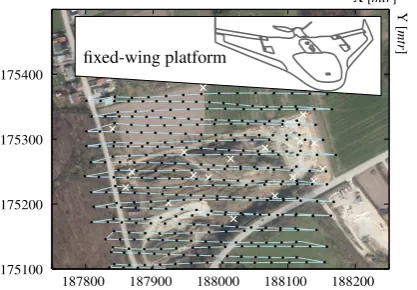
For the demonstration of this assessment we conducted a case study over an open mine near the villages of Kiezegem and Meensel, Belgium. This relatively small excavation site has a total cover-age of0.19km2, and elevation differences up to18meter, see
figure 1 & 2. A large part of the mine was overgrown with vege-tation, while the Eastern part was open bare sand. On this part of the mine a steep sandy wall up to seven meters is situated.
2.1 Ground truth
Control points consisted of twenty one targets. We chose for 33x33 cm wooden plates painted with a single checkerboard pat-tern, attached to a pole which was firmly hammered into the ground. Targets were measured with GNSS RTK, a polygonal net of total station measurements and some closed loops acquired through digital levelling. The processing of the data were inte-grally adjusted (Boekelo, 1996), based on the statistical princi-ples of the Delft school in the Move3 software package (version 4.2). The estimated standard deviation of the target points were horizontally all around three millimeter and vertically around half a millimeter.
2.2 Platforms and Instruments
The flights were done on 6th and 9th of August 2013, at the same time of the day, with the aim of delivering the same product in sense of ground sampling distance (GSD). Two different types of UAVs flew over the open mine, namely a Gatewing UX5 and a Microdrone MD4-1000, the platform and instrument specifica-tions are given in Table 1. These systems are commercially avail-able in these settings, their different properties are due to design decisions.
flight. This is in contrast to the multi-rotor system which has a stall speed of an order smaller. Consequently, different acquisi-tion strategies are taken.
Trimble Microdrone
UX5 MD4-1000
type fixed-wing multi-rotor
camera NEX-5R NEX-7
focal length 24 19 [mm]
sensor width 23.4 23.4 [mm]
sensor height 15.6 15.6 [mm]
resolution 16.0 24.0 [Mpix]
height 75 70 [mtr]
GSD 0.024 0.017 [mtr]
overlap 75 80 [%]
sidelap 85 45 [%]
exposure 1/2000 1/400 [sec]
setting shutter priority manual sensitivity automatic manual white balance automatic automatic
calibrated 2 2
collimator 2 2
Table 1: Acquisition details of the two different platforms and flight specifications during the case study.
175100 175200 175300 175400
fixed-wing platform
Y
[
mtr
]
187800 187900 188000 188100 188200 X [mtr]
Figure 1: Orthophoto of the open mine, with black dots illustrat-ing the acquisition centers (a total of 360 is used), the ground control points are indicated with a white cross.
The multi-rotor stabilizes the camera by hovering the platform and a stabilization rig underneath. This makes time available to adjust the sensitivity (through ISO) and integration time (through shutter time) during operation. Its operation strategy is struc-tured, its flight path is defined before hand, and executed as best as possible in this way. Its rotors make a full control possible over the three spatial dimensions, thus its position can be adjusted until the UAV has arrived at the predefined point. Due to its stabiliza-tion rig images are taken at close to perfect nadir and inline of the direction of flight. This results in close to ideal stereo imagery, for stereo plotting. In addition, the operator sets the ISO value and integration time. The flight resulted in six strips and a total of 148 images, taken in 16 minutes from roughly 70 meters above the surface.
The fixed-wing platform has a more ad-hoc flight planning, its flight path is decided in the field. The most favorable direction of flight is with wind from the side. Wind directions can be very local, therefore the orientation of the strips is determined just be-fore take-off. The platform glides in the air due to its wings and delta-shape, it has an efficient combustion. Hence, it can cover
large areas, as it has a cruising speed of 80 km/h and an opera-tion time of 45 minutes. However, the camera is fixed within the body, thus adjustment of the camera orientation is not possible. In addition the images have a crab angle, and the flight strips are not perfectly parallel. Nonetheless, at 75 meters above ground the system can still collect imagery with an high overlap. In or-der to make this possible, the ISO value is changed automatically, with the shutter time fixed. In our case, there was only a slight breeze, thus multiple configurations could be flown. From one of such a flight 360 images were selected, acquired at an approxi-mate height of 75 meter above the ground.
The two cameras are both manufactured by Sony, but have dif-ferent specifications. The camera attached to the fixed wing has bigger pixels of 4.76µm, in respect to the other (3.9µm), but a lower resolution. In addition, the fixed wing has a Voigtl¨ander lens which is assembled with the help of a collimator. The other system uses a normal consumer grade lens. In the remainder of this paper we will verify if these significant differences in instru-mental quality pay off.
175000 175100 175200 175300 175400
X [mtr]
Y
[
mtr
]
tiepoint acquisition
multi-rotor platform
187800 187900 188000 188100 188200 Figure 2: Large scale map, in Lambert72projection, illustrating the neighborhood of the site. The black dots (148) indicate the position of the UAV when a photo was taken. The crosses illus-trate the used ground-points for its assessment.
2.3 Processing
Both data-sets were processed with Pix4Dmapper software (ver-sion 1.1.23). This photogrammetric software package calibrates the camera as an integral part of the bundle adjustment. Its pro-jected errors are calculated through least squares adjustment us-ing the full covariance matrix of internal and external parameters (Strecha, 2014). The input of the geometric quality of the con-trol points is independent of its coordinate axis, therefore three millimeter was assigned to all entries. Furthermore, the software presumably derives a gray-scale image through a weighted mean of (0.2126, 0.7152, 0.0722) for the three colorbands (R,G,B), as is given in the camera database of the software. Due to the clear checkerboard pattern of the control points we assume we can identify the markers on pixel to sub-pixel level.
3 METHODS
as the one dataset has automatic camera settings unlike the other. For the image motion we look at the translational or rotational blur within the imagery, which are rooted from the fast cruising speed and/or turbulence of the air. We look at the quality of both lenses, by assessing the absolute and relative radial distortion, in grayscale as well as seperate colorbands. Furthermore, the dis-persion or chromatic abberation, is estimated. The used method-ologies will be explained hereafter.
3.1 Intensity
To extract a quality indicator for the acquired imagery a his-togram over the whole population of images might give a hand-hold. Both campaigns are flown on the same time of day, the sky having a bit of overcast sky in the form of alto-cumulus. Ideally, all the color histograms should be flat with a uniform occurence of each gray value. Skewted curves might indicate wrong settings of aperture and shutter time, or monotonous reflection distribu-tion pattern on the ground. Furthermore, we checked individual images for absence of contrast or saturation of pixel regions.
3.2 Image motion
Another difference between both systems is the image motion during operation. For the fixed-wing configuration the shutter speed of the camera is typically 1/2000 of a second, resulting in 1.1 cm platform movement during acquisition. While the ground sampling resolution is in the same order as this upper bound, therefor the possibility exist that image blur would be significant. This is done by estimating the blur kernel within a single image, following (Fergus et al., 2006), based on the following model:
B=K⊗L+N (1)
HereBdenotes the original image corrupted with blur,Kis the kernel which describes the local motion of the camera position and orientation,Lrepresents the ideal or latent image andNis white noise, this convolutional concept is also illustrated in fig-ure 3. Here the sum of the blur kernel adds up to unity. Within equation 1 only the original image is given. To further constrain the estimation a-priori variance information is included. Its vari-ance model is based on a Gaussian mixutre model, as a distri-bution with heavy tails is assumed in this natural image. This is used in a blind deconvolution estimation, where the blur kernel is estimated with a maximum marginal probability (Miskin and MacKay, 2000). A seven pixel wide square kernel was given as free space, and the intiated kernel had three elements within a row.
K
⊗ =
L B
Figure 3: Visual illustration of the blur convolution. At the left the original or pure image (L), is convoluted with the blur kernel (K). Here the brightness intensity of this matrix is related to value intensity, where the brightest value corresponds to0.1. The result of the convolution (B) is illustrated on the right.
For the case of a prominent translational motion, this kernel would hold for the entire image. However, for rotational motion, the ker-nel content would vary depending on its location within the im-age. In (Whyte et al., 2012) such an advanced rotational model is implemented, following the same estimation procedure as in equation 1. However, for the fixed-wing case the translation is presumably a more prominent factor than its rotational compo-nent, while the multi-rotor might experience both effects. There-fore, we estimated a local kernel subdividing the image into small patches, giving the possibility to extract the dominant motion (movement or rotation) from the image by inspection.
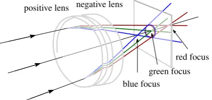
3.3 Refraction
The light rays traveling through the optics of the camera are bound to Snellius’ law. Different lenses and coatings are placed in-line to let all visible wavelength eventually coincide on the imaging plane to resemble a pinhole model. Nonetheless, discrepancies occur, thus green is taken as reference by focussing this wave-length sharply on the imaging plane (Bass et al., 2009). Con-sequently, wavelengths situated in the other two colorbands will not perfectly coincide, as is illustrated in figure 4. This results in image blur and is known as longitudal abberation. For light enter-ing at an off-nadir angle, a different effect is observed, beenter-ing pe-ripheral color shift. This is due to the wavelength dependent foci that result in different maginifications away from the center and is known as lateral abberations. Wide angle lenses, such as fish-eye, can have pixel displacements up to pixels (Schwalbe and Maas, 2006). Equally, for consumer-grade camera’s this pixel displace-ment is in the range of 0.1 to 0.2 (Cronk et al., 2006). Conse-quently, a pinhole and lens distortion model do not describe the chromatic aberrations working on the imaging plane.
The inclusion of chromatic aberrations within the camera calibra-tion has already been stressed by (Remondino and Fraser, 2006). This is certainly relevant in UAV photogrammetry, where the con-strain of instrument weight, favors the use of compact camera’s. But more importantly, the quality of lenses is low, thus chromatic aberrations can be a problem (Kaufmann and Ladst¨adter, 2005). Especially for the use of mapping, as mixed bands seems to be used for the detection of features within the imagery. Due to the mixing of bands, such features are smoothed, resulting in bad localization. To make matters worse, chromatic aberrations are greatest at the sides, while at the same time measurements on this periphery do strengthen the triangulation.
positive lens negative lens
blue focus green focus
red focus
In our case two different optical systems and specifications were used. On the multi-rotor platform a consumer grade lens was at-tached, while on the fixed wing a professional lens was deployed. Thus a difference in lens design in the form op different coatings and glass of the optics influences the amount of chromatic abber-ations, hence its image quality. In addition, the latter lens was adjusted with a collimator and its depth of field was set to a range of about 100 meters. Now it is of interest to see if such effort is worth the investment of money and time. To assess this we take two different approaches: On the one hand, individual bands are processed and the estimated calibration is evaluated. This gives an idea about the amount of radial distorition of each chromatic band and might give inference about the effect of refraction and the aid of a collimator.
On the other hand, the pheripherial colorshift effect is directly estimated on the imagery, in a similar fashion as (Kaufmann and Ladst¨adter, 2005). The relative displacement (the vectorc, with componentsdx, dy) is estimated for different colorbands. This proxy of colorshift gives a direct indication of the effect of chro-matic aberration and the use of a collimator. To come back to the compact camera case, such estimation could be of great use. They can function as extra input for advanced lens-models that take the chromatic aberrations into account. Such information is only present during acquisition, as the movement of lens to camera body make the lens model different from flight to flight. This effect is not only limited to consumer-grade cameras with moveable lenses, but the fixed-wing platform seem to change its internal parameters due to the shock inflicted during take-off and landing.
What is different from out approach in respect to (van den Heuvel et al., 2006, Luhmann et al., 2006), is the high amount of auto-matic processing and the lack of calibration targets. We use a bulk of imagery and estimated independent of contrast its displace-ment. For this the software package of COSI-Corr was used to estimate the color-shift on sub-pixel level (Leprince et al., 2007). It uses the phase shift within the frequency domain of the agery to estimate the displacement. However, in this domain im-age matching estimates between the red and the blue bands can give bad results. This is probably due to the methodology used within COSI-Corr, where the normalization of intensities is not implemented in the frequency domain, thus resulting in less ro-bust result than a normalized cross-correlation in the spatial do-main (Heid, 2012). Therefore, the red to blue band combination was estimated in the spatial domain through normalized cross correlation (NCC). The other colorbands were assumed to have enough a strong spectral covariance between each other, andesti-mated in the frequency domain.
However, an individual image might be corrupted with noise, or have unreliable matches, therefore weighting can be applied over the bulk of imagery (k). This is done through the use of the sig-nal to noise ratio (SNR) value, also given with the displacement estimation. This figure of merit ranges from 0 to 1, and to put more value to higher matches the weighting is done by the square of this value. Thus for every subset within the imagery the dis-placement vector is calculated through:
dx=
Additionally to the individual estimation of relative displacement,
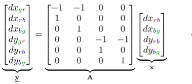
the estimation can also be conditioned. This is done by the vec-tor addition property of the chromatic abberation, where the dis-placement of all color-shift vectors should form a closed triangle:
0 =cgr+crb+cbg wherec⊤= [ dx dy ] (3)
Rearraning these terms gives the following model,
This linear system of equations can be solved by least sqaures adjustment following (Teunissen, 2000).
4 RESULTS & DISCUSSION
The methodology given in the former section will now be used to assess the three criteria, that is, intensity, motion and refraction. Both datasets are processed with all ground points. The total is more than necessary; the control points were respectively 224 and 558 times measured in the imagery. Thus this redundancy can be of use for the optimization of internal camera parameters.
To assess these criteria the dataset needs to be of high quality, therefor we looked at the projection errors of the photogrammet-ric processing. Heretofore, a minimum of six points is used for the bundle block adjustment, with others set as verification. The resulting re-projection errors on these points are given in table 2. This gives a clear insight in the strength of the block itself, and from these results we assume the extra control points will mostly be used to benefit the internal estimation. Its results are consider-ably better then other studies (Harwin and Lucieer, 2012), (Haala et al., 2013), but we attribute that to the inclusion of traditional surveying of the control points.
x σx y σy z σz
wing [mm] 3.3 17.9 10.2 32.2 27.8 26.4
rotor [mm] 2.2 10.2 2.7 13.4 56.1 41.4
Table 2: The mean and standard deviation of the re-projection error of control points in millimeters over three dimensions for the two datasets, using a population of 16 and 12, respectively.
4.1 Intensity
The normalized histograms of the two image datasets is given in figure 5. It clearly shows a skewed distribution for the blue band to the lower end. Both camera had automatic white balance, from the EXIF data it seems as all settings were similar. The only difference was a manual exposure setting, in comparision to a shutter priority for the fixed-wing sensor. This might explain the discrepancy in the blue range.
uniform distribution. Especially on the higher end of the quanti-zation level, however a closer look on individual images did show saturated areas and regions of low contrast. A strong transition from vegetation to bare sand did saturate the camera in images, as shown in the example of figure 6. This is a small drawback, how-ever this local effect was only visible in when the normal vecotr of the terrain was directed to the camera. Thus there is no loss of topographic information, as neighboring imagery showed enough contrast to triangulate this region. This is one of the big advan-tages of multiview UAV photogrammetry (Haala et al., 2013). Though only0.019hof the entire dataset is saturated, these pix-els were mostly located on the sandy area. Nevertheless, this flight was conducted with the application to mine management. The rest of the site is mostly covered by vegetation, with minimal saturation and good contrast.
Overall, it seems to be better to use the automatic adjustment for the sensitivity settings, as the dynamic range of a frame cam-era is limited. Changes in direct sun light, caused by clouds, needs dynamic adjustment to be able to fly during such condi-tions. The drawback of this choice is a less contrastrich picture, as the weight of these histograms lay in the lower digital numbers.
4.2 Image motion
For both flight campaigns we estimated the blur kernel over square patches of 200 pixels wide, this was done to extract a global trend due to turbulence during acquisition or through adjustment of the stabilization rig. A result of such an estimation is illustrated in figure 7. The estimated blur kernel is seven pixels wide, but for our case the estimation mostly resolved in one peak element in the order of 0.5 and some surrounding elements. Thus half of the energy of the ideal image falls within one pixel, the rest is smeared out over the others. In the illustration this maximum is taken as the center, with its surrounding kernel elements. If the maximum was on the border it is translated to that side.
A local pattern is observable: low or distributed kernel values over homogenous terrain, such as paved road. Apart from that, the kernels extracted from the fixed-wing platform do have a ten-dency to the direction of flight. On the other hand, the multi-rotor dataset resulted in kernel estimates with noisy or at least random distribution of one pixel wide. No global trend related to rota-tional effects were identifiable. Thus, although some distortion is observed in the fixed-wing platform, the image blur is of similar size for both systems. This might be adressed to the longer shutter
50 100 150 200 250
0 0.002 0.004 0.006 0.008 0.010
multi-rotor platform P(·)
DN fixed-wing platform
blue greenred
Figure 5: Normalized histogram of digital numbers (DN) for dif-ferent color channels. The population came from 300 images for the fixed-wing configuration and 148 for the multi-rotor platform.
200 400 600 800 1000
100
200
300
400
500
Figure 6: Subset of saturated image, the red dots indicate pixels with fully saturated intensity. On the left bright sand is visible as well, however this is part of the sand wall and its normal is not directed to the camera.
flight direction
Figure 7: A subset of the center from a fixed-wing acquisition, imposed its estimated blur kernels. Furthermore, on the top mid-dle a control point (checkerboard) is indicated by a red circle.
time of the multi-rotor, where accumulation of rotational motion and displacement for the multi-rotor is four times larger. Such a long shutter speed is caused by the smaller pixel size, needing more time to collect as much light as the fixed-wing system.
From this we can conclude that the fixed-wing system is at its lower limit, concerning operation height. The reverse is true for the multi-rotor, mostly due to the pixel size.
4.3 Refraction
For the two datasets all bands are separately adjusted within an integrated bundle adjustment, its resulting internal parameters are given in table 3. Unfortunately, the impact in the form of error propagation is lacking in the table due to the missing variance es-timation.
The camera underneath the multi-rotor was calibrated before-hand, using a calibration board. Among others, the focal length (18.964) and principle point (−0.076,0.012) are off from the es-timated parameters. However, assuming that these a-priori values are better than the estimated parameters is non-trivial. Namely, the calibration of the camera is done on close-range, hence the depth of field and ray-tracing is considerably different than the acquisition situation.
focal principle point radial distortion tangential distortion y
RGB 23.750 0.01088 0.00814 -0.35237 0.48328 -0.25109 -3.88195 10.10892
red 23.805 0.00202 0.04336 -0.35587 0.50926 -0.28843 -3.35373 9.59824
green 23.780 0.00250 0.04361 -0.35556 0.50683 -0.28000 -3.34017 9.32285
blue 23.785 0.00372 0.04570 -0.35593 0.51241 -0.28666 -3.41274 9.25690
RGB 18.953 0.05041 -0.00773 -1.53304 5.40636 -5.64330 -8.55423 5.86782
red 18.971 0.05261 -0.00755 -1.52956 5.44092 -5.87893 -8.73146 6.64479
green 18.969 0.05044 -0.00677 -1.53217 5.45597 -5.89284 -8.08861 6.73982
blue 18.971 0.05267 0.00765 -1.54016 5.51681 -6.07598 -8.17524 6.10410
Table 3: Internal calibration estimations for different colorbands. The first half is rooted from the fixed-wing campaign, the second half is originated from imagery of the multi-rotor. The imagery on the right indicates the coordinate axis for the principle point and illustrates the different kind of distortions. The radial and tangential parameters should be applied to metric radial distance.
Voigtl¨ander lens has far less radial distortion, in addition, its val-ues are more stable than for the other camera. The only exception is the principle point of the full color processing, which is out off sync with the other values, its not easily identifyable. No signif-icant difference is present for the tangential components, which would suggest the unimportance of a collimator.
Nevertheless, the estimated internal parameters from table 3 are used to estimate a theoretical displacement between both images, these are illustrated aside of the measured estimates in the figure 8. The directional lines give the orientation of the displacement, while the color indicates the displacement in pixelsize, the results are smoothed with an mean kernel of 10 pixels in size.
3.84 11.54 19.24
Figure 8: Color-shift estimation in pixels modelled for the red to green colorband of the fixed-wing system.
For the second part, the estimation of chromatic aberration di-rectly on the images, 148 and 114 images were processed, each with 36 pixel wide block sizes. The results from some combina-tions are illustrated in figure 9,10. Here the estimation is based on equation 2. Including the other estimates, as with equation 4, was not applied, as the matching within the frequency domain was far off from a radial pattern. This might be due to the great ammount of vegetation within the imagery, which results in different reflec-tion values in each band (Kaufmann and Ladst¨adter, 2005). Fur-thermore, due to storage limitations in the UAV’s, all images are compressed through JPEG, which is unfavorable for the detection of chormatic abberation (Cronk et al., 2006). Nonetheless, a pat-tern in both images is visible, and as we took a large sampling set we expect this compression to be of minimal influence.
The measured pixel displacement is an order different then the theoretical estimate. Some radial patterns are visible (looking at the colorscale), but it is far from linear. Not only with respect to the modelled abberations, but also inbetween both measured images. Futhermore, the radial magnitude does seem to have an osscilating pattern, this is partially visible in the modeled case,
nonetheless the modelled displacement is an order in size to big and not in such frequency.
This illustrates the create complexity of the lens system. Assum-ing, a simple system as illustrated in figure 4, contradicts the in-dividual estimations of the focal lengths in table 3. An more ap-proriate workflow would be the extraction of these abberations before processing and still adopting a simple pinhole model.
From these results we can conclude that a collimator may not be worth the effort, nevertheless investing in better optics does result in less distortion. However, for chromatic abberations the consumer-grade camera seem to perform on a similar level or even slightly better.
5 CONCLUSIONS AND FUTURE WORK
In this work we assess different UAV mapping systems through comparing the quality of the collected imagery. The two
map-3.84 11.54 19.24
Figure 9: Color-shift estimation in pixels rooted from sub-pixel normalized cross=correlation (NCC) measurements for the red to blue colorband of the fixed-wing system.
3.14 9.43 15.72 22.01
ping strategies: ad-hoc and fast flown, or structured but slower are completely different and resolve in different instrumental choices. However, the resulting products are of similar resolution. There-for we assessed three different components of acquisitioning to show the pro and cons of both systems. Nonetheless, our results could be strengthend by consequently isolating each individual system components and look at its effect.
Firstly, manually setting camera sensitivity and shutter time needs experience and knowledge of the camera system. It gives imagery with high contrast, though it introduces a chance of saturation. If one wants to stay on the save side, an automatic setting should be chosen, however this does influence the contrast.
Concerning flight speed and elevation, this size of the site in re-spect to resolution seems to be close to the system’s tipping point. For mapping of areas of several hectares, a fixed-wing platform seems to be more effective than a multi-rotor platform. It can ac-quire imagery with ultra high resolution, with a similar amount of blur as the multi-rotor. On the other hand, if a higher resolution is needed, the multi-rotor can be more suited for this task. Fur-thermore, the acquisition of long streched terrain is favoured over such small terrain, as the image taking of both systems are at a similar rate. This is due to the turning of the fixed-wing platform.
An investment in a better lens does seem to produce less distorted imagery and better estiamtion of its parameters. Nonetheless, as software transforms these images to grayscale, its improvement is immersed below the noiselevel. The effect of a collimator is not directly visible, thus might not be worth the calibration effort. The estimation of chromatic aberrations directly on the imagery seems possible. However, some improvements with respect to precision and robustness is possible and needed. For commer-cial easy to use software, there is a need for (co-)variance indica-tion. This is of great help for interpretation of the results from the integrated estimation of internal and external orientation. This is in line with (Chandler et al., 2005), how proposes to drop radial terms if its significance can only marginally be detected. It however contradicts other popular structure-from-motion soft-ware how do give the opportunity to estimate a forth term for the radial distortion (R4). However, as has been shown, lens
mod-els do not describe the measured patterns, thus overfitting seems to occur. The correction of imagery before its processing seems profitable and its automatic implementation is work in progress.
ACKNOWLEDGEMENTS
The authors would like to thank Orbit Geospatial solutions and Gatewing NV for the services of flying the campaigns over the project area. Furthermore we acknowledge Maarten Borremans and Dries Van Velthoven for assistance during fieldwork. This research was funded by the Institute for the Promotion of Inno-vation through Science and Technology in Flanders (IWT Vlaan-deren). It is a part of the 3D photogrammetry for surveying engi-neering (3D4Sure) project.
REFERENCES
Bass, M., DeCusatis, C., Enoch, J., Lakshminarayanan, V., Li, G., Macdonald, C., Mahajan, V. and Van Stryland, E., 2009. Handbook of optics, Volume II: Design, fabrication and testing, sources and detectors, radiometry and photometry. McGraw-Hill, Inc.
Boekelo, G., 1996. Adjustment models and mapping. Hydro-graphic Journal pp. 3–8.
Chandler, J., Freyer, J. and Jack, A., 2005. Metric capabilities of low-cost digital cameras for close range surface measurement. The photogrammetric record 20(109), pp. 12–26.
Cronk, S., Fraser, C. and Hanley, H., 2006. Automatic metric cal-ibration of colour digital cameras. The photogrammetric record 21(116), pp. 355–372.
Eisenbeiss, H. and Sauerbier, M., 2011. Investigation of UAV systems and flight modes for photogrammetric applications. The Photogrammetric Record 26(136), pp. 400–421.
Fergus, R., Singh, B., Hertzmann, A., Roweis, S. and Freeman, W., 2006. Removing camera shake from a single photograph. In: ACM Transactions on Graphics, Vol. 25, ACM, pp. 787–794.
Haala, N., Cramer, M. and Rothermel, M., 2013. Quality of 3D points clouds from highly overlapping UAV imagery. Interna-tional Archives of Photogrammetry, Remote Sensing and Spatial Information Sciences XL-1/W2, pp. 183–188.
Harwin, S. and Lucieer, A., 2012. Assessing the accuracy of georeferenced point clouds produced via multi-view stereopsis from unmanned aerial vehicle (UAV) imagery. Remote Sensing 4, pp. 1573–1599.
Heid, T., 2012. Deriving glacier surface velocities from repeat optical images. PhD thesis, University of Oslo.
Kaufmann, V. and Ladst¨adter, R., 2005. Elimination of color fringes in digital photographs caused by lateral chromatic aberra-tion. In: Proceedings of the XX International Symposium CIPA, Vol. 26, pp. 403–408.
Leprince, S., Barbot, S., Ayoub, F. and Avouac, J.-P., 2007. Auto-matic and precise orthorectification, coregistration, and subpixel correlation of satellite images, application to ground deformation measurements. Geoscience and Remote Sensing, IEEE Transac-tions on 45(6), pp. 1529–1558.
Luhmann, T., Hastedt, H. and Tecklenburg, W., 2006. Mod-ellierung der chromatischen aberration in bildern digitaler auf-nahmesysteme. Photogrammetrie, Fernerkundung und Geoinfor-mation 5, pp. 417–425.
Miskin, J. and MacKay, D. J. C., 2000. Ensemble learning for blind image separation and deconvolution. In: M. Girolani (ed.), Advances in Independent Component Analysis, Springer-Verlag.
Remondino, F. and Fraser, C., 2006. Digital camera calibra-tion methods: consideracalibra-tions and comparisons. In: Internacalibra-tional Archives of Photogrammetry, Remote Sensing and Spatial Infor-mation Sciences, Vol. XXXVI-5, pp. 266–272.
Remondino, F., Barazzetti, L., Nex, F., Scaioni, M. and Sarazzi, D., 2011. UAV photogrammetry for mapping and 3D model-ing current status and future perspectives . In: International Archives of Photogrammetry, Remote Sensing and Spatial Infor-mation Sciences, Vol. XXXVIII-1, pp. 1–7.
Schwalbe, E. and Maas, H.-G., 2006. Ein ansatz zur elimina-tion der chromatischen aberraelimina-tion bei der modellierung und kalib-rierung von fisheye-aufnahmesystemen. In: T. Luhmann and C. M¨uller (eds), Photogrammetrie, Laserscanning, Optische 3D-Messtechnik, Beitrge der Oldenburger 3D-Tage, pp. 122–129.
Strecha, C., 2014. Pix4D error estimation. Technical report, Pix4D knowledge base, Lausanne, Switzerland.
van den Heuvel, F., Verwaal, R. and Beers, B., 2006. Calibra-tion of fisheye camera systems and the reducCalibra-tion of chromatic abberation. In: International Archives of Photogrammetry, Re-mote Sensing and Spatial Information Sciences, Vol. XXXVI-5, pp. 1–7.