SHAPE DISTRIBUTION FEATURES FOR POINT CLOUD ANALYSIS
- A GEOMETRIC HISTOGRAM APPROACH ON MULTIPLE SCALES
R. Blomleya,∗, M. Weinmanna, J. Leitloffa, B. Jutzia
a
Institute of Photogrammetry and Remote Sensing, Karlsruhe Institute of Technology (KIT),
Englerstr. 7, 76131 Karlsruhe, Germany -{rosmarie.blomley, martin.weinmann, jens.leitloff, boris.jutzi}@kit.edu
Commission III, WG III/4
KEY WORDS:LIDAR, Point Cloud, Features, Geometric Feature Design, Multiscale, Probability Histogram
ABSTRACT:
Due to ever more efficient and accurate laser scanning technologies, the analysis of 3D point clouds has become an important task in modern photogrammetry and remote sensing. To exploit the full potential of such data for structural analysis and object detection, reliable geometric features are of crucial importance. Since multiscale approaches have proved very successful for image-based ap-plications, efforts are currently made to apply similar approaches on 3D point clouds. In this paper we analyse common geometric
covariancefeatures, pinpointing some severe limitations regarding their performance on varying scales. Instead, we propose a different
feature type based onshape distributionsknown from object recognition. These novel features show a very reliable performance on a wide scale range and their results in classification outnumbercovariancefeatures in all tested cases.
1 INTRODUCTION
Contemporary laser scanning systems provide 3D point clouds with increasing accuracy and point density that may contribute significantly to the huge potential of remote sensing in environ-mental applications. Therefore there is a growing need for effi-cient 3D geometric characterisation, structural analysis and inter-pretation of such data.
Depending on the application, supervised and unsupervised clas-sification approaches may be pursued, yet all of them rely on de-scriptive features. Following techniques well-known from im-age processing, the analysis of invariant moments has been ap-plied to study the geometric properties of 3D point cloud data (Maas and Vosselman, 1999). In particular, second-order mo-ments, represented by the covariance matrix or structure tensor (West et al., 2004) are increasingly popular in geometric feature extraction (Jutzi and Gross, 2009; Toshev et al., 2010; Niemeyer et al., 2012). A good overview of currently used features for 3D point cloud analysis and a comprehensive study of their classifi-cation relevance is given by Chehata et al. (2009) and Mallet et al. (2011). These features can be grouped into height-based fea-tures, geometric features derived from covariance or local plane estimations and sensor specific features such as full-waveform or echo-based features. In those studies, height-based features are generally ranked very important. Geometric features such as co-variance and local plane features have to be calculated from a certain local neighbourhood around each point in question. In fact, according to scale selection studies (Demantk´e et al., 2011; Gressin et al., 2012), those features perform best when calculated from a particularly homogeneous neighbourhood determined by optimisation of the local dimensionality-based entropy.
Meanwhile, landscape classification tasks usually involve some recognition of complex structures beyond the reach of small ho-mogeneous neighbourhoods. This has led to a change in image-based remote sensing towards object-image-based and multiscale meth-ods (Blaschke and Hay, 2001; Hay et al., 2005), which is not yet
∗Corresponding author.
common in point cloud analysis. Object-based point cloud stud-ies include shape parameterisations similar to 3D Hough trans-formations (Vosselman et al., 2004) and grouping of points to segments and entities (Reitberger et al., 2009; Xu et al., 2012). Multiscale approaches on point cloud data are often very time-consuming due to their iterative schemes, when the appropriate neighbourhood is sought locally (Pauly et al., 2003; Mitra and Nguyen, 2003; Demantk´e et al., 2011). Especially in natural en-vironments, an evaluation of multiple scales can prove benefitial as it accounts for the characteristic scales of different structures (Brodu and Lague, 2012).
In remote sensing applications, point cloud analysis is sometimes limited by the number of returns per area, due to which important details may not be resolved. However, it has been pointed out very early that both in cases with object sizes larger than the given resolution and object sizes smaller than the resolution, some char-acteristic spatial autocorrelation can be expected (Strahler et al., 1986). Thus probabilistic distributions of geometric properties in 3D point clouds may hold more information than locally calcu-lated parameters. Reaching beyond locally homogeneous neigh-bourhoods, histogram distributions have already been success-fully used in computer vision sciences (Tombari et al., 2010). In image-based keypoint description, the SIFT algorithm is a prominent example for robustness and effectiveness achieved by a set of local histograms (Lowe, 2004). In 3D point clouds, exist-ing histogrammetric approaches are limited to surface keypoint description, as they rely on surface normal vectors (Tombari et al., 2013; Rusu et al., 2009).
In Section 2, the main conceptual components of this approach are set out. Even though height features are of paramount im-portance for real applications (Chehata et al., 2009; Mallet et al., 2011), they will not be included in the following investigations. For the sake of clarity, only rotation-invariant geometric features (like those in the original shape distributionproposal) will be compared. For practical purposes, the improvement achievable by height-based features should be independent of the features discussed here and would be beyond the scope of this paper. Section 3 briefly describes the conducted experiments based on commonly available urban area benchmark data. Any findings obtained here are discussed in Section 4. First of all, the results of scale investigations using theshape distributionfeatures are eval-uated. Secondly, a comparison with presently well-established
covariancefeatures is conducted. This comparison covers
Sup-port Vector Machine classifications at multiple scales, an estima-tion of the entropy-based optimum neighbourhood size for these features (Demantk´e et al., 2011) and a feature relevance assess-ment (Weinmann et al., 2013). Finally, the novel features’ per-formance is evaluated and compared against thecovariance fea-tures’ result.
2 METHODOLOGY
The first part of the proposed methodology (Section 2.1) is in-tended to illustrate the need for a novel geometric feature type suitable for multiscale investigations. Section 2.2 therefore cov-ers both a current geometric feature set (Section 2.2.1) and the concept of this novel approach (Sections 2.2.2 and 2.2.3). Since our investigations focus on feature design, classification methods are only used to evaluate the features practical performance and are therefore discussed in the experimental part.
2.1 Scale Investigations
In geometric point cloud analysis, any single observation (ele-ment) can only be interpreted by its relationship to other elements and its probability of belonging to a certain object class. Yet any object class displays characteristic coherence at different spa-tial scales (Hay et al., 2005). Therefore it is crucial to establish features that can represent structural characteristics on multiple scales. Features calculated on some scales may reproduce spe-cial autocorrelation characteristics that are not observed at other scales. A multiscale approach should therefore lead to enhanced classification results. For classification, one or more scales have to be determined, at which the sampling pattern of the sensor can resolve unique properties of the object class in question. Some approaches utilize a scale space representation for this purpose. Since this is not trivial for 3D cases (Tombari et al., 2013), we clarify that we use scale as a neighbourhood size parameter only.
Moreover, the shape of the considered neighbourhood has to be chosen carefully (Filin and Pfeiffer, 2005). For the purpose of aerial laser scanning (ALS), a cylindrical neighbourhood is found to be preferable, as it allows the features to capture the height dis-tribution of the surrounding point cloud (Shapovalov et al., 2010). The varying cylinder radii to be investigated are chosen as2n/2
m withn ∈ Nand−4≤ n≤ 11. Thereby all possibly resolved structural scales should be covered, as the radius ranges between 0.25 m (within the lateral placement accuracy of the laser scan-ner) and 45 m (above most object sizes). However, the features that will be presented in Section 2.2.2 are easily adapted to dif-ferent laser scanning applications, as they are insensitive to the overall neighbourhood shape.
2.2 Feature Design
Feature design is of central importance to every knowledge rep-resentation and classification. In the following section a widely used geometric feature type for point cloud analysis will be in-troduced to point out some of its important properties (Section 2.2.1). Subsequently a novel geometric feature type will be in-troduced, first describing its origin in object recognition (Section 2.2.2) and afterwards a further contribution for its adaption as feature for classification applications (Section 2.2.3).
2.2.1 Covariance Features. Most present approaches using 3D geometric features employ features derived from the local covariance matrix representing second-order invariant moments within the point positions. The covariance matrix is calculated fromNobservationsA1,2,3as follows:
[Cov]ij= PN
l=1(Ai−Ai)·(Aj−Aj)
N , (1)
wherei, j ∈[1,2,3]andAiholds the mean of all observations
in the respective dimension. Subsequent principal component analysis is used to determine linearly uncorrelated second-order moments in an orthogonal eigenvector space. The correspond-ing eigenvaluesλ1,2,3 then hold a great potential to calculate local features including dimensionality (linearity, planarity and sphericity) and other measures such as omnivariance, anisotropy and eigenentropy. The eigenvalues, sorted asλ1≥λ2≥λ3≥0 and the measures listed in Equation 2, will be referred to as
co-variancefeatures.
Linearity: Lλ=λ1λ−1λ2 Planarity: Pλ= λ2λ−1λ3
Sphericity: Sλ=λλ31 Omnivariance: Oλ=
3 √
λ1λ2λ3 Anisotropy: Aλ=λ1λ−1λ3
Eigenentropy: Eλ=−P3i=1λiln(λi) Sum ofλs: Σλ=λ1+λ2+λ3 Change of curvature: Cλ= λ1+λλ32+λ3
(2)
Yet it is especially important for these features to be derived from a suitably chosen neighbourhood size. It is the nature of second-order moments that the distance of one element from the mean contributes quadratically (c.f. Equation 1) and therefore elements in the vicinity are far less important than those further away. Since the principal component analysis is an orthogonal and thereby unitary transformation, the resulting eigenvalues are sen-sitive to the original scaling. Demantk´e et al. (2011) and Gressin et al. (2012) show evidence that a suitable spherical neighbour-hood size can be found by minimization of the Shannon entropy based on dimensionality-features. Yet it remains to be shown if this optimum neighbourhood size forcovariancefeatures corre-sponds to the characteristic scale of any structure. To advance fur-ther research in the field, ofur-ther geometrical features more suited to multiple scales are indispensable.
2.2.2 Shape Distributions. The characteristic scale of com-plex and partially random structures may not always be identical to the optimum neighbourhood size ofcovariancefeatures. Yet to reveal such patterns, a statistical distribution of randomly sam-pled values may be more suitable than single values such as
co-variancemeasures. Therefore we adapt a concept proposed and
• D1: distance between any random point and the centroid of all considered points,
• D2: distance between two random points,
• D3: square root of the area of a triangle between any three random points,
• D4: cubic root of the volume of a tetrahedron between any four random points,
• A3: angle between any three random points.
In the practical implementation presented in Sections 3.3 and 3.4, the resulting values will be calledshape values. The resulting histogram therefore represents the probability distribution of the taken geometric measures within the observed sample and should reveal repeating structures by a more frequent occurrence of some values. By this approach, feature extraction is reduced to a simple random sampling procedure. Such features are fast to calculate, mirror- and rotation-invariant and robust regarding outliers, noise and varying point density due to application-specific scanning or flight patterns. Notably, classification steps thereafter resemble a comparison of the probability distributions of these simple geo-metric measures.
2.2.3 Adaptive Histogram Binning. Dissenting from the originalshape distributionproposal, we use an adaptive histogram binning approach to achieve maximum variance of significant ob-servations from the gross of the total dataset. Above all, this step ensures a scale-independent performance. For this purpose, a simple histogram equalization procedure, known from image processing applications (Gonzales and Wood, 2002), is adapted. For all measured values at a linear binning scopemk, withk =
0, ..., L−1andLthe number of bins, a transformation function
T(mk)to a non-linear binning scope is found in such a way that
a histogram of any large number of random samples is equally distributed. The transformation function is defined as
T(mk) = k
X
j=0
pm(mj), (3)
wherepmis defined as the probability of occurrence of a value
withinmkfrom a large number of samplesn:
pm(mk) = nk
n , (4)
wherenkis the number of occurrences withinmk.
3 EXPERIMENTS
To test the proposed features on commonly accessible data, a benchmark dataset is evaluated. Due to the fundamental nature of our investigations and the exclusive use of geometric features, results will not be compatible to others already published in the benchmark context. We aim to submit classification results in-cluding other features for evaluation in future work and therefore focus on internal evaluation only. The overall experimental pro-cedure, featuring used data (Sections 3.1 and 3.2), feature cal-culation (Sections 3.3 and 3.4), as well as classification (Section 3.5), will be presented here, before results are discussed in Sec-tion 4.
3.1 Benchmark Dataset
To test the performance of this genuine feature type, an ALS dataset contained in the ISPRS benchmark on urban classification at the Vaihingen test site (Cramer, 2010) is used. This data was
acquired in August 2008 with a Leica ALS50 system at a mean flying height of 500 m with a45oviewing angle, 30 % overlap of
flight strips and a mean point density of 4pts./m2 .
3.2 Reference Data and Point Cloud Access
In order to test the features’ performance by supervised classifi-cation, some ground truth reference is mandatory. Voxel-based reference data was obtained from Gerke and Xiao (2014), and reference points were selected as those data elements closest to the centre of each voxel. The four classes and their respective number of elements are:
16·104
points for building roofs 7·104
points for trees 6·104
points for vegetated ground 12·104
points for sealed ground
For easy access to all point cloud elements contained in a cylin-drically shaped neighbourhood around each element at different radii, ak-dimensional tree structure is used.
3.3 Shape Value Calculation
As we pursue random sampling, some limitations have to be set. Thus we limit ourselves to 255pulls of geometric shape val-uesper histogram. This limits computational efforts and mini-mizes the possible impact of varying point densities within the dataset. For a cylindrical neighbourhood in the given data50% of all points have this number of neighbours at a cylinder radius of∼2.5 m, suggesting that this number should allow for a repre-sentative description. For big neighbourhoods, a relatively small percentage of all points in the volume element are thereby consid-ered. This prevents false high recognition values due to overlap between the neighbourhood of adjacent points and overfitting in reference areas smaller than the considered neighbourhood.
Moreover the number of bins per shape histogram has to be spec-ified. A large number of bins will allow for sophisticated neigh-bourhood descriptions, but for a small amount of points the sig-nature may then not be descriptive. Therefore we decide to use 10 bins per shape histogram in this proposal, yet an optimization of both bin and sampling number may still be sought in future investigations.
3.4 Histogram Binning Thresholds
To avoid arbitrary threshold selection and ensure a balanced per-formance ofshape distributionsat multiple scales, an automated choice of histogram binning thresholds (Section 2.2.3) is imple-mented. Random samples are taken at each radius, and the cor-respondingshape valuescollected for adaptive binning calcula-tion. After500pulls, no significant change of the adapted binning thresholds is observed. Those thresholds are used thereafter to
formshape distributionsfromshape valuessampled within each
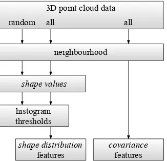
neighbourhood, as described in Section 2.2.2 and Figure 1.
3.5 Classification
Since our investigations focus on feature design, we aim for a simple, commonly used and universal classification procedure, knowing that better results may be achieved by other methods in the field. Furthermore, the chosen classifier should ideally be tolerant to irrelevant and redundant attributes, which may be sig-nificant as a large number of feature values is used in the present histogram approach. Considering those requirements, Support
3D point cloud data
neighbourhood
shape values
histogram thresholds
shape distribution
features
covariance
features all
random all
Figure 1: Feature calculation workflow. To calculateshape distri-butionfeatures, histogram binning thresholds have to be acquired first as described in Section 3.4.
use, generally produce very accurate results and cope well with possible correlation between features (Kotsiantis, 2007).
To investigate whether some classes are particularly well described by features from certain scales, separate one-against-all distinctions are better suited than one multiclass classifica-tion. The identification of each separate class is performed using a one-against-all binary SVM classifier provided by the LIBSVM package (Chang and Lin, 2011). The classifier uses a radial basis function kernel and depends on two parameters, namelyγ, rep-resenting the width of the Gaussian kernel function andC, a soft margin parameter allowing for some misclassifications. To en-sure a smooth classification procedure, all feature data are scaled to a range between zero and one. A grid search for optimal val-ues ofγandCis completed by evaluation of the cross-validation accuracy on a threefold partition of the training data. The grid search and subsequent training of a classifier with the best re-spective parameters is performed on a subset containing1,000 data points of each class to avoid a bias by unbalanced reference data distribution. Afterwards, the performance of any selected classifier is tested on all labelled training data (4.1·105
points).
4 EVALUATION
A central enquiry within our work, namely an analysis ofshape distributionfeatures at different scales, will be presented in Sec-tion 4.1. Afterwards the same analysis is conducted based upon commonly usedcovariancefeatures in Section 4.2.1. This com-parison is supported by an estimation of the dimensionality-based optimum neighbourhood forcovariancefeatures (Section 4.2.2) and classifier-independent feature relevance assessment for both feature types (Section 4.2.3). Eventually, the best classification results of both geometric feature types are evaluated on point cloud level in Section 4.3. Shape distributionresults are visu-alised at different settings to analyse the overall performance.
4.1 Scale Analysis
The classification procedure described in Section 3.5 is performed for all four classes contained in the reference data. Features are calculated from different sizes of the cylindrical neighbourhood around each point, as described in Section 3.3 and 3.4.
To ensure consistency and compatibility with other leading pub-lications, each classification result is evaluated using the metrics
described by Rutzinger et al. (2009):Completeness,correctness
andqualityare calculated from the number of correctly identified (TP), correctly rejected (TN), falsely identified (FP) and falsely rejected (FN) elements.
Comp. = TP
TP+FN (5)
Corr. = TP
TP+FP (6)
Quality = 1 1
/Comp.+1/Corr.−1 (7)
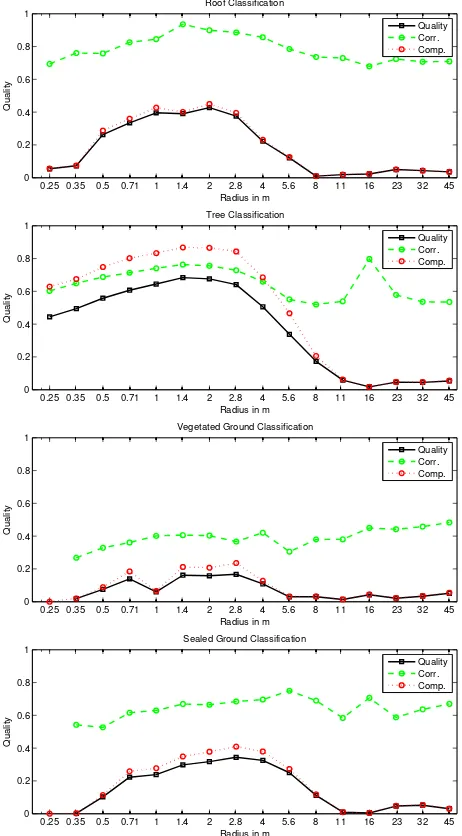
The application of such metrics allows for an in-depth analysis of the classification results and a precise comparison of the fea-tures’ performance on different classes. Classification results for all investigated neighbourhood sizes are presented in Figure 2.
As the resulting graphs are smooth and generally display an even peak-like distribution, it is presumed thatshape distribution fea-tures are a suitable choice to evaluate geometrical properties of point clouds over a wide spatial neighbourhood scale. No promi-nent peaks occur to suggest a strong pattern or scale preference for individual classes in this data. Optimal results are achieved at the following neighbourhood radii:
2.0m for roofs 1.4m for trees
2.8m for vegetated ground 2.8m for sealed ground
Interestingly all those maxima fall within a similar range. This generally descriptive size forshape distributionfeatures is signif-icantly higher than the neighbourhood size used forcovariance
features in ALS. The values of 1.0 m used by Jutzi and Gross (2009) and 0.75 m used by Niemeyer et al. (2012) agree well with findings presented later in Section 4.2.2. Yet a suitable scale may well depend on the feature type chosen. When pursuing a covari-anceapproach, homogeneous surroundings at a smaller scale will cause more distinctive features, whereasshape distributionsmay rather show repeating or significant patterns at a larger scale.
Comparing different classes, it is notable that trees are detected with the highestcompletenessbut slightly lowercorrectnessand perform best in regard to quality. For all other classes, cor-rectnessis higher thancompleteness. This indicates, that rela-tively few points are misassigned, but several points are missed. Whereas for roofs and sealed ground a reasonable amount is still detectable, vegetated ground performs significantly lower due to both lowcompletenessandcorrectness.
4.2 Comparison with Covariance Features
Linearly independent second-order invariant momentsλ1≥λ2≥
λ3 ≥ 0and features calculated from them as described in Sec-tion 2.2.1, are derived for the whole range of neighbourhood sizes around each point. Prior to classification, all features are rescaled so that all but 1 % of outliers lie between zero and one.
4.2.1 Comparison of Scale Analysis. Using exclusively co-variancefeatures, it is not possible to conduct a cohesive analysis spanning the same scale range as shown forshape distribution
0.25 0.35 0.5 0.71 1 1.4 2 2.8 4 5.6 8 11 16 23 32 45
Figure 2: Evaluation of classification results exclusively employ-ingshape distributionfeatures for different neighbourhood sizes. Quality measures are calculated according to Section 4.1 and plotted against the radius of a cylindrical neighbourhood.
well with findings published in (Niemeyer et al., 2011), where
covariancefeatures are used among others.
A very intriguing observation is to be seen at large neighbourhood sizes, where quality increases dramatically. Yet this increase can-not be said to result from a generally better classification perfor-mance. BothCandγparameters of the SVM are very high for these results, indicating an overfitting (Kotsiantis, 2007). This can be explained by a high overlap between the neighbourhood of points within the same reference area, as the reference areas are much smaller than the neighbourhood for feature calculation. As explained in Section 2.2.1,covariancefeatures are highly in-fluenced by elements far away from the mean of all observations. For a homogeneous point distribution in the area, the extra num-ber of points in a bigger circle increases more than quadratically by the increase of radius, and the distance of all those extra points in turn contributes quadratically to the covariance matrix. There-fore the neighbourhood of relatively close points has a huge over-lap and the resulting features are nearly identical, causing the ob-served overfitting. Further studies, taking only a reduced random
0.25 0.35 0.5 0.71 1 1.4 2 2.8 4 5.6 8 11 16 23 32 45
Figure 3: Evaluation of classification results exclusively
employ-ing covariancefeatures for different neighbourhood sizes. As
explained in Section 4.2.1 the quality increase above 16 m radius is not reliable outside of reference areas.
subset per neighbourhood forcovariancecalculation, did not dis-play an increase incompletenessandqualityfor high neighbour-hood radii but were otherwise identical. Therefore increased clas-sification quality for radii above 16 m is regarded as erroneous.
Generally the classification results based oncovariancefeatures are less smooth than those determined fromshape distribution
features. Rooftops could perform best at 8 m, but not as good as theshape distributionresult. Sealed ground shows a spike at 2 m, reaching a similar result to theshape distributions. Trees are best detected at lower radii, but not as well as when usingshape distributions, and vegetated ground is virtually un-detectable.
4.2.2 Dimensionality-Based Scale Selection. Following an argument stated in (Demantk´e et al., 2011), the optimum local neighbourhood size may be found by minimizing the absolute value of the Shannon entropy based on dimensionality covari-ancefeatures:
0.25 0.35 0.5 0.71 1 1.4 2 2.8 4 5.6 8 0.2
0.4 0.6 0.8 1
Radius in m
Classwise Mean Entropy
Roof Tree Veg. G. Seal G.
Figure 4: Classwise mean Shannon entropy calculated according to Equation 8 for different neighbourhood sizes.
For radii below 16 m the classwise mean Shannon entropy, ignor-ing ill-defined values due toλi = 0, is shown in Figure 4. For
trees, there is no mimimum to be found, wheras for other classes a slight minimum occurs at a neighbourhood radius of 0.5 m. Due to the limited point density of the data set however, no feature separation can be achieved on this scale.
4.2.3 Comparison of Feature Relevance. To further evalu-ate our features’ performance independent of the used classifica-tion scheme, a filter-based feature relevance assessment is per-formed. The procedure follows (Weinmann et al., 2013). Seven filter-based feature relevance measures are evaluated, each result-ing in a relevance ratresult-ing for all elements of the feature vector. In this case 61 feature vector elements have to be compared (5shape
distributiontypes with 10 feature values each and 11covariance
features). The applied score functions evaluate the relation be-tween the values of a feature vector element for all observations and the respective class labels. Tested measures arecχ from a χ2
independence test, the Fisher scorecFisher describing the ra-tio of interclass and intraclass variance, the Gini IndexcGinias a statistical dispersion measure, the Information Gain measure
cIGrevealing the dependence in terms of mutual information, the Pearson correlation coefficientcPearsonderived from the degree of correlation between a feature and the class labels, the ReliefF measurecReliefFrevealing the contribution of a certain feature to the separability of different classes, and thectmeasure derived from at-test for checking how effective a feature is for separating different classes.
Since all relevance measures follow different metrics, the value for relative importance was deduced from the ranking order among all feature vector elements. Afterwards, the mean of all importance values was taken for every feature vector element, re-sulting in a mean importance. A value of one would be achieved if a feature vector element was rated the most important feature by all relevance measures, and zero if it was always rated least important. The mean of all mean importance values belonging to one feature type group is plotted in Figure 5. To avoid any bias by unbalanced reference data, a subset containing 1,000 points per class is investigated.
Comparing the five differentshape distributiontypes, all printed as slashed lines, it is clearly seen that the angle between any three random points A3 is only weakly descriptive at those neighbour-hood radii that showed the best classification performance in Sec-tion 4.1. The volume between any four random points D4 is of great importance here. Obviously the different classes in this test could be best separated by distinctive probability distributions of
0.25 0.35 0.5 0.71 1 1.4 2 2.8 4 5.6 8 11 16 23 32 45
0 0.1 0.2 0.3 0.4 0.5 0.6 0.7 0.8 0.9 1
Radius in m
Feature Mean Importance
A3 D1 D2 D3 D4 Cov.
Figure 5: Mean rank of mean feature relevance per feature group for different neighbourhood sizes. A3, D1, D2, D3 and D4 are the
shape distributionfeatures described in Section 2.2.2, and Cov.
thecovariancefeatures as described in Section 4.2.
random volumetric measures. However, at very small scales, an-gular and lower dimensional measures like D1, D2 and D3 are of more importance.
As forcovariancefeatures, a different behaviour can be observed. Below∼3 m the importance is roughly the same as for D1, D2 and D3shape distributionfeatures. The slight peak in importance at 0.71 m corresponds well to the optimum neighbourhood size derived from entropy measures (c.f. Figure 4). For higher radii a steep increase followed by high constant importance is measured. This corresponds directly to the scale at which the performance of
shape distributionfeatures decreases in the SVM classifications
(c.f. Figure 2).
4.3 Internal Evaluation on Point Cloud
As the approach with varying scales implies that distinctive neigh-bourhood sizes may be class-dependent, four separate classifica-tion results from different best neighbourhood sizes (c.f. Sec-tions 4.1 and 4.2.1) have to be considered. Combining these sep-arate results necessitates the choice between complete labelling and higher label accuracy. Since the chosen subset of classes may not be complete, we choose only to regard elements with a label probability higher than 50 % as labelled. Therefore some elements may not belong to any class. Also, some points may be found belonging to two or more classes. In this case, the la-bel probability is weighted by the quality of the respective binary classifier before choosing the maximum result.
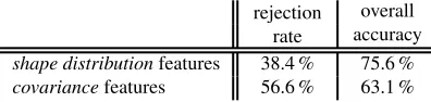
4.3.1 Quantitative Evaluation. An evaluation was conducted for bothshape distributionandcovariancefeatures. Rejection rate (percentage of unidentified elements) and overall accuracy of both results each combined from four binary classifications are shown in Table 1. In this regard theshape distributionfeatures obviously outperform thecovariancefeatures, since the rejection rate is significantly lower whilst the overall accuracy is increased. Not only can more elements be identified, but also more of these elements are identified correctly.
rejection rate
overall accuracy
shape distributionfeatures 38.4 % 75.6 %
covariancefeatures 56.6 % 63.1 %
known pred. Roof Tree Veg. G. Seal. G. Comp.
Roof 77530 10094 4036 6749 78.8 %
Tree 1052 61474 80 47 98.1 %
Veg. G. 4983 4271 8576 11493 29.2 %
Seal. G. 6994 3771 8634 45032 69.9 %
Corr. 85.6 % 77.2 % 40.2 % 71.1 %
Quality 69.6 % 76.1 % 20.4 % 54.4 %
known pred. Roof Tree Veg. G. Seal. G. Comp.
Roof 31544 37225 0 10993 39.5 %
Tree 1040 46941 0 78 97.7 %
Veg. G. 2867 7073 0 13101 0 %
Seal. G. 4699 10306 0 41953 73.7 %
Corr. 78.6 % 46.2 % - 63.4 %
Quality 35.7 % 45.7 % - 51.7 %
Table 2: Confusion matrices of combined classification results usingshape distribution(top) andcovariance(bottom) features, ignoring all cases in which an element could not be detected in any of the classes.
For a more extensive analysis of the different classes’ perfor-mance, the resulting confusion matrices as well ascompleteness,
correctnessand quality are shown in Table 2. The most
sig-nificant increase is observed for the detection of building roofs, wherequalityalmost doubles, mainly due to an increase in com-pleteness. The significantqualityincrease for trees is mainly due to increasedcorrectness, whereas sealed ground is detected with comparablequality. Vegetated ground lacks a comparison, as it can not be detected at all bycovariancefeatures.
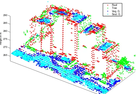
4.3.2 Qualitative Analysis. Figures 6 and 7 depictshape dis-tributionclassification results as coloured point clouds for qual-itative analysis in particular areas. Both the gable roof and tree visible in Figure 6 are generally well classified. Only minor er-rors occur at the ridge of the roof, where some points are mis-taken for vegetated ground, and at the rim of the roof, where some points are misclassified as tree. This is in good agreement with the findings of Figure 2, indicating that trees are generally covered by greatcompleteness, butcorrectnessis lacking. The high-rise buildings depicted in Figure 7 show a misclassification of flat roofs as sealed and vegetated ground. This is not surpris-ing, asshape distributionsdo not incorporate knowledge about a predominant direction. Therefore, a flat roof and its edge to the ground have the very same characteristics as flat ground and the adjoining edge of a house. Except for the existing confusion between sealed and vegetated ground, those examples explain all main off-diagonal contributions to the confusion matrix.
These misclassification examples demonstrate, that classification results are expected to increase significantly by the use of other, non-geometric features and especially by height distribution fea-tures. The latter should enhance results dramatically, since it in-troduces a predominant direction and avoids the confusion be-tween building roofs and ground. Therefore an evaluation in the benchmark context is intended in a future extended approach.
5 DISCUSSION
At first glance, a main shortcoming of the proposed approach seems to be the high amount of points that cannot be assigned to any class in the evaluated benchmark case. Yet this is inherent in the exclusive examination of their rotation invariant geometrical context without prior assumptions about a predominant direction or a knowledge-based interpretation of man-made objects.
280 285 290 295 300
Height in m
Roof Tree Veg. G. Seal. G.
Figure 6: Gable roof and adjacent trees, generally well labelled solely according to geometricshape distributionfeatures.
265 270 275 280 285 290
Height in m
Roof Tree Veg. G. Seal. G.
Figure 7: High-rise buildings. Without the use of further features, flat roofs are mistaken as ground.
The class-dependent scale investigations in this urban area con-text did not yield novel insights about structural characteristics. On the one hand this may be different for other applications, for example in structural vegetation analysis. On the other hand, a combination of different scale features in a unified approach may also enhance classification results for point clouds. For example, the findings of the conducted feature relevance assessment sug-gest a combination of angular A3 features at very small neigh-bourhood sizes with volumetric D4 features at ranges between 0.5 m and 16 m around each point in question for this dataset. Broad multiscale studies might be an alternative to extensive ap-proaches optimising the size of every local neighbourhood.
6 CONCLUSION AND OUTLOOK
In this papershape distributionsare introduced as a new feature type for geometric point cloud analysis, that outperforms com-patible existing features. As they resemble a histogram approach, they require more feature vector elements, yet they hold the po-tential to describe structures beyond the relatively small reach of homogeneous neighbourhoods well described bycovariance fea-tures. This is especially important when the point density is lim-ited, as in the case of aerial laser scanning data.
In future work we plan to optimise the feature design for remote sensing applications. We aim to combineshape distribution fea-tures from multiple scales as well as other feafea-tures types such as height distributions and full-waveform features. Especially vege-tation analysis represents a promising field of application for mul-tiscale approaches. Effective classification schemes such as ran-dom forests, boosting algorithms or Markov ranran-dom fields may be used to further enhance classification results.
ACKNOWLEDGEMENTS
The Vaihingen data set was provided by the German Society for Photogrammetry, Remote Sensing and Geoinformation (DGPF) (Cramer, 2010):http://www.ifp.uni-stuttgart.de/dgpf/ DKEP-Allg.html.
The authors would like to thank Markus Gerke for providing la-belled reference data for training and internal testing.
References
Blaschke, T. and Hay, G. J., 2001. Object-oriented image analysis and scale-space: Theory and methods for modeling and evaluating multiscale landscape structure. International Archives of Photogrammetry and Re-mote SensingXXXIV, Part 7/W5, pp. 22–29.
Brodu, N. and Lague, D., 2012. 3D terrestrial lidar data classification of complex natural scenes using a multi-scale dimensionality criterion: Applications in geomorphology.ISPRS Journal of Photogrammetry and Remote Sensing68, pp. 121–134.
Chang, C.-C. and Lin, C.-J., 2011. LIBSVM: A library for support vec-tor machines. ACM Transactions on Intelligent Systems and Technology 2(3), pp. 27:1–27:27. Software available athttp://www.csie.ntu. edu.tw/~cjlin/libsvm.
Chehata, N., Guo, L. and Mallet, C., 2009. Airborne lidar feature selec-tion for urban classificaselec-tion using random forests.International Archives of Photogrammetry, Remote Sensing and Spatial Information Sciences XXXVIII, Part 3/W8, pp. 207–212.
Cramer, M., 2010. The DGPF test on digital aerial camera evaluation -overview and test design.Photogrammetrie - Fernerkundung - Geoinfor-mation2, pp. 99–115.
Demantk´e, J., Mallet, C., David, N. and Vallet, B., 2011. Dimensionality based scale selection in 3D lidar point clouds. International Archives of Photogrammetry, Remote Sensing and Spatial Information Sciences XXXVIII, Part 5/W12, pp. 97–102.
Filin, S. and Pfeiffer, N., 2005. Neighborhood systems for airborne laser data.Photogrammetric Engineering and Remote Sensing71(6), pp. 743– 755.
Gerke, M. and Xiao, J., 2014. Fusion of airborne laserscanning point clouds and images for supervised and unsupervised scene classification. ISPRS Journal of Photogrammetry and Remote Sensing87, pp. 78–92.
Gonzales, R. C. and Wood, R. E., 2002.Digital Image Processing. 2. edn, Prentice-Hall, Upper Saddle River, NJ, chapter Histogram Equalization, pp. 91–95.
Gressin, A., Mallet, C. and David, N., 2012. Improving 3D lidar point cloud registration using optimal neighborhood knowledge.ISPRS Annals of the Photogrammetry, Remote Sensing and Spatial Information Sciences I, Part 3, pp. 111–116.
Hay, G. J., Castilla, G., Wulder, M. A. and Ruiz, J. R., 2005. An auto-mated object-based approach for the multiscale image segmentation of forest scenes. Internation Journal of Applied Earth Observation and Geoinformation7, pp. 339–359.
Jutzi, B. and Gross, H., 2009. Nearest neighbor classification on laser point clouds to gain object structures from buildings. International Archives of Photogrammetry, Remote Sensing and Spatial Information SciencesXXXVIII, Part 1-4-7/W5, pp. 207–213.
Kotsiantis, S. B., 2007. Supervised machine learning: A review of clas-sification techniques.Informatica31, pp. 249–268.
Lowe, D. G., 2004. Distinctive image features from scale-invariant key-points.International Journal of Computer Vision60, pp. 91–110.
Maas, H.-G. and Vosselman, G., 1999. Two algorithms for extracting building models from raw laser altimetry data. ISPRS Journal of Pho-togrammetry and Remote Sensing54, pp. 153–163.
Mallet, C., Bretar, F., Roux, M., Soergel, U. and Heipke, C., 2011. Rele-vance assessment of full-waveform lidar data for urban area classification. ISPRS Journal of Photogrammetry and Remote Sensing66, pp. 71–84.
Mitra, N. J. and Nguyen, A., 2003. Estimating surface normals in noisy point cloud data. Proceedings of the Annual Symposium on Computa-tional Geometry,pp. 322–328.
Niemeyer, J., Rottensteiner, F. and Soergel, U., 2012. Conditional random fields for lidar point cloud classification in complex urban areas. ISPRS Annals of the Photogrammetry, Remote Sensing and Spatial Information SciencesI, Part 3, pp. 263–268.
Niemeyer, J., Wegner, J., Mallet, C., Rottensteiner, F. and Soergel, U., 2011. Conditional random fields for urban scene classification with full waveform lidar data. In: Stilla, U., Rottensteiner, F., Mayer, H., Jutzi, B., Butenuth, M. (Eds.),Photogrammetric Image Analysis, ISPRS Con-ference - Proceedings. Lecture Notes in Computer Science, Vol. 6952, Springer, Heidelberg, Germany, pp. 233–244.
Osada, R., Funkhouser, T., Chazelle, B. and Dobkin, D., 2002. Shape distributions.ACM Transactions on Graphics21(4), pp. 807–832.
Pauly, M., Keiser, R. and Gross, M., 2003. Multi-scale feature extraction on point-sampled surfaces.Computer Graphics Forum22(3), pp. 81–89.
Reitberger, J., Schn¨orr, C., Krzystek, P. and Stilla, U., 2009. 3D seg-mentation of single trees exploiting full waveform LIDAR data. ISPRS Journal of Photogrammetry and Remote Sensing64, pp. 561–574.
Rusu, R. B., Blodow, N. and Beetz, M., 2009. Fast point feature his-tograms (FPFH) for 3D registration. Proceedings of the IEEE Interna-tional Conference on Robotics and Automation,pp. 1848–1853.
Rutzinger, M., Rottensteiner, F. and Pfeifer, N., 2009. A comparison of evaluation techniques for building extraction from airborne laser scan-ning. IEEE Journal of Selected Topics in Applied Earth Observations and Remote Sensing2(1), pp. 11–20.
Shapovalov, R., Velizhev, A. and Barinova, O., 2010. Non-associative Markov networks for 3D point cloud classification. International Archives of Photogrammetry, Remote Sensing and Spatial Information SciencesXXXVIII, Part A, pp. 103–108.
Strahler, A. H., Woodcock, C. E. and Smith, J. A., 1986. On the nature of models in remote sensing. Remote Sensing of Environment20, pp. 121– 139.
Tombari, F., Salti, S. and Di Stefano, L., 2010. Unique signatures of histograms for local surface description. In: Daniilidis, K., Maragos, P., Paragios, N. (Eds.),ECCV 2010, Part III. Lecture Notes in Computer Science, Vol. 6313, Springer, Heidelberg, Germany, pp. 356–369.
Tombari, F., Salti, S. and Di Stefano, L., 2013. Performance evaluation of 3D keypoint detectors.International Journal of Computer Vision102, pp. 198–220.
Toshev, A., Mordohai, P. and Taskar, P., 2010. Detecting and parsing architecture at city scale from range data.Proceedings of the IEEE Con-ference on Computer Vision and Pattern Recognition,pp. 398–405.
Vosselman, G., Gorte, B. G. H., Sithole, G. and Rabbani, T., 2004. Recog-nising Structure in Laser Scanner Point Clouds. International Archives of Photogrammetry, Remote Sensing and Spatial Information Sciences XXXVI, Part 8/W2, pp. 33–38.
Weinmann, M., Jutzi, B. and Mallet, C., 2013. Feature relevance as-sessment for the semantic interpretation of 3D point cloud data. ISPRS Annals of the Photogrammetry, Remote Sensing and Spatial Information SciencesII, Part 5/W2, pp. 313–318.
West, K. F., Lersch, J. R., Pothier, S., Triscari, J. M. and Iverson, A. E., 2004. Context-driven automated target detection in 3-d data.Proceedings of SPIE5426, pp. 133–143.