A note on the causal relationship between
energy and GDP in Taiwan
Hao-Yen Yang
UDepartment of Economics, Shih-Hsin Uni¨ersity, No. 1, Line 17, Mu-Cha Rd. Sec. 1, Taipei 116, Taiwan
Abstract
This paper re-examines the causality between energy consumption and GDP by using updated Taiwan data for the period 1954]1997. As a secondary contribution, we investigate the causal relationship between GDP and the aggregate as well as several disaggregate categories of energy consumption, including coal, oil, natural gas, and electricity. Applying Granger’s technique, we find bidirectional causality between total energy consumption and GDP. We find further that different directions of cause exist between GDP and various kinds of energy consumption.Q2000 Elsevier Science B.V. All rights reserved.
JEL classification:Q41 Keywords:Energy; GDP
1. Introduction
Ž .
In a recent article in this journal Cheng and Lai 1997 , using the version of
Ž .
Hsiao 1981 of the Granger’s causality method, found unidirectional causality running only from GDP to energy consumption for the period of 1955]1993 for Taiwan. Their results imply that increasing economic growth requires enormous consumption of energy, yet there are many factors contributing to economic
Ž .
growth, and energy is but one part of it Cheng and Lai, 1997 .
The purpose of this paper is to re-examine the causality between energy consumption and GDP by using updated Taiwan data for the period 1954]1997. As
U
Tel.:q00-886-2-2236-8225 ext. 548; Fax:q00-886-2-2236-1658.
Ž .
E-mail address:[email protected] H. Yang
0140-9883r00r$ - see front matterQ2000 Elsevier Science B.V. All rights reserved.
Ž .
a secondary contribution, we investigate the causal relationship between GDP and the aggregate as well as several disaggregate categories of energy consumption, including coal, oil, natural gas, and electricity. Applying Granger’s technique, we find bi-directional causality between total energy consumption and GDP. This implies that energy shortage may restrain the economic growth in Taiwan. Further, we find that different directions of cause exist between GDP and various kinds of energy consumption.
In the following section, the methodology and models that we employ in the causality tests are briefly presented. Further sections report results obtained from Granger’s causality tests, and explain why it differs from the results of study by
Ž .
Cheng and Lai 1997 .
2. Methodology
The first attempt at testing for the direction of causality was proposed by
Ž .
Granger 1969 . Granger’s test is a convenient and very general approach for detecting the presence of a causal relationship between two variables. A time series
ŽX. is said to Granger-cause another time series Ž .Y if the predication error of current Y declines by using past values of X in addition to past values of Y. The application of the standard Granger’s causality test requires that the series of variables to be stationary. Therefore, two variables are first transformed to covari-ance stationary processes. This is done by taking their first differences. The
Ž .
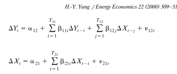
Phillips]Perron test Phillips and Perron, 1988 is used in examining the unit roots and stationary property of two variables. To test for Granger’s causality between energy consumption and GDP, two bivariate models are specified, one of energy consumption and another for GDP. If two variables are stationary, the standard form of the Granger’s causality test can be specified accordingly as follows:
T11
OIL y1.5163 y5.2384
U
GAS y1.2259 y3.5576
U
ELEC 2.0021 y5.0561
U
Signification at the 10% level. The critical value of the Phillips]Perron statistic at the 10% level is
Ž .
T11 T12
whereDis the difference operator,Ytand Xt are GDP and energy consumption,T
is the number of lags,a andb are parameters to be estimated, andnt is the error
Ž . Ž . Ž . Ž .
term. Eqs. 2 and 4 are in unrestricted forms, while Eqs. 1 and 3 are in
Ž . Ž .
restricted forms. But Eqs. 1 and 2 are made a pair to detect whether the coefficients of the past lags of the energy consumption can be zero as a whole. By
Ž . Ž .
the same token, Eqs. 3 and 4 are made other pair to detect whether the coefficient of the past lags of GDP can be zero as a whole. Stated differently, if the
Ž .
estimated coefficient on lagged values of X in Eq. 2 is significant, it means that it explains some of the variance of Y that is not explained by lagged values of Y
itself. This indicates that X is causally prior to Y and said to Granger-cause Y.
Ž .
Similarly, if the estimated coefficient on lagged values of Y in Eq. 4 is significant, it means that it explains some of the variance of X that is not explained by lagged values of X itself. This indicates that Y is causally prior to X and said to Granger-cause X. Therefore, F statistics are calculated to test whether the coeffi-cients of lagged values can be zero.
Ž .
According to Engle and Granger 1987 , if two variables are co-integrated, then a more comprehensive test of causality, which has become known as an error-cor-rection model, should be adopted. In this procedure, X Granger cause Y, if either the estimated coefficients on lagged values of X or the estimated coefficient on lagged value of error term from co-integrated regression is statistically significant. Similarly,Y Granger-cause X, if either the estimated coefficients on lagged values of Y or the estimated coefficient on lagged value of error term from co-integrated
Table 2
The critical value of the Phillips]Perron statistic at the 10% level is approximately y3.50 see
regression is statistically significant. The inclusion of lagged value of error term from co-integrated regression in the error-correction model gives an extra avenue through which the effects of causality can occur. Therefore it is necessary to test for the co-integration property of the energy consumption and GDP.
The causal results are sensitive to the lag structure of the independent variables. The arbitrariness in choosing lags can distort the estimates and yield misleading
Ž . Ž .
causality inferences. Hsiao’s 1981 procedure combines the Akaike 1969 final
Ž . Ž .
prediction error FPE Akaike, 1969 criterion with Granger’s causality test will be employed in this study to guide the selection of the appropriate lag specifications.
Ž .
Hsiao’s procedure consists of two steps. The first step is to estimate Eq. 1 to
Ž .
compute the residual sum of squares by varying the lag order t11 from 1 toT11.
Ž . Ž U.
The smallest FPE t11 decides the optimal lag t11 . The second step is to estimate
Ž . Ž .
Eq. 2 . For additional variable X, one varies again the lag order t12 from 1 toT12
Ž U .
and calculates the modified FPE. Also, the smallest FPE t11, t12 decides the
Ž U.
optimal lag t12 . Once the appropriate lags are determined, an alternative way of testing the direction of causality is compared the smallest FPEs of the
aforemen-ŽU U
. Ž U
.
tioned step’s one and two. If FPE t11, t12 is smaller than the FPE t11 , it implies that energy consumption Granger-cause GDP. Subsequently, causality from GDP to energy consumption may also be estimated by repeating the same procedure for
Ž . Ž .
Eqs. 3 and 4 .
3. Data and empirical results
3.1. Variable definition and data sources
In order to investigate whether there is a causal relationship between energy
Table 3
Granger’s causality tests between GDP and ENERGY
a
FPE represents Akaike’s 1969 final prediction error.
UU
Table 4
Granger’s causality tests between GDP and COAL
a
FPE represents Akaike’s 1969 final prediction error.
UU
Signification at the 5% level.
U
Signification at the 10% level.
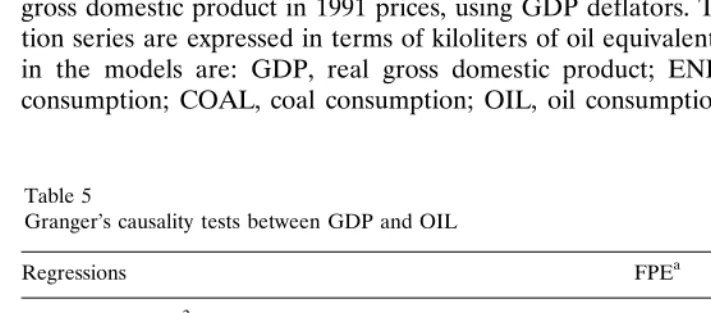
consumption and GDP, data covering the period 1954]1997 are used. The nominal gross domestic product series in Taiwanese currency are transformed into real gross domestic product in 1991 prices, using GDP deflators. The energy consump-tion series are expressed in terms of kiloliters of oil equivalent. The variables used in the models are: GDP, real gross domestic product; ENERGY, total energy consumption; COAL, coal consumption; OIL, oil consumption; GAS, natural gas
Table 5
Granger’s causality tests between GDP and OIL
a
FPE represents Akaike’s 1969 final prediction error.
UU
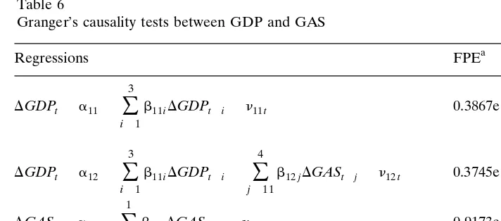
Table 6
Granger’s causality tests between GDP and GAS
a
FPE represents Akaike’s 1969 final prediction error.
U
Signification at the 10% level.
consumption; ELEC, electricity consumption. All the variables used in this study are compiled from the AREMOS economic-statistic data-banks, created jointly by the Ministry of Education and National Taiwan University in Taiwan.
3.2. Results from unit-roots and co-integration tests
Table 1 reports unit-root tests for the series of all variables, including GDP,
Table 7
Granger’s causality tests between GDP and ELEC
a
FPE represents Akaike’s 1969 final prediction error.
UU
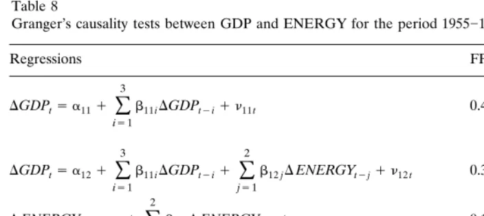
Table 8
Granger’s causality tests between GDP and ENERGY for the period 1955]1993
a
FPE represents Akaike’s 1969 final prediction error.
UU
Signification at the 5% level.
ENERGY, COAL, OIL, GAS, and ELEC. The Phillips]Perron test provides the formal test for unit roots and stationarity in this study. As shown in Table 1, the Phillips]Perron values of all the variables are less than the critical value ofy3.13 at the 10% level. This indicates that the series of all the variables are non-sta-tionary. However, non-stationarity can be rejected for the series of all the variables at the 10% level when first-differenced data are used. Hence, the Granger’s causality models are estimated with first-differenced data.
As stated previously, if GDP and energy consumption are non-stationary and the linear combination of the series of two variables is non-stationary, then standard Granger’s causality test should be adopted. But, if GDP and energy consumption are non-stationary and the linear combination of the series of two variables is stationary, then error-correction modelling should be adopted. Therefore it is necessary to test for the co-integration property of the series of GDP and energy consumption before performing the causality test. Table 2 reports co-integration test for the series of GDP and energy consumption. As shown in Table 2, the Phillips]Perron values are less than the critical value of]3.50 at the 10% level for all cases. This reveals that the GDP and both aggregate and disaggregate cate-gories of energy consumption are not co-integrated. Therefore, the standard
Ž . Ž .
Granger’s causality test is applicable, as shown in Eqs. 1 ]4 .
3.3. Results from Granger’s causality tests
structures were chosen by Akaike’s final prediction error criterion. The results of Granger’s causality test between GDP and both the aggregate and the disaggregate categories of energy consumption are presented in Tables 3]7. Table 3 reports causality between GDP and ENERGY. As shown in Table 3, it reveals that for the GDP equation, since 0.3867eq10)0.3284eq10, we accept the hypothesis that ENERGY Granger-cause GDP. This means that the inclusion of past values of ENERGY in the GDP equation provided a better explanation of current values of GDP than when excluded. Conversely, for the ENERGY equation, since 0.1279e
q13)0.1021eq13, we conclude that GDP Granger-cause ENERGY. This means that the inclusion of past values of GDP in the ENERGY equation provided a better explanation of current values of ENERGY than when excluded. Furthermore, as shown in Table 5, ENERGY in GDP equation and GDP in ENERGY equation are statistically significant at the 5% level, implying that there is bi-directional causality between total energy consumption and GDP.
Tables 4]7 report causality between GDP and various kinds of energy consump-tion. As shown in Tables 4]7, it is noteworthy that bi-directional causal linkages between GDP and both coal and electricity consumption are identified. But a unidirectional causality running from GDP to oil consumption and a unidirectional causality running from natural gas consumption to GDP are detected for this case. We find that different directions of cause exist between GDP and various kinds of energy consumption.
3.4. Discussion of the empirical results
Ž .
The finding of this paper does not support the findings of Cheng and Lai 1997 of unidirectional causality running from GDP to total energy consumption for Taiwan. The difference in the results of this study and that of Cheng and Lai may be attributable to the choice of the sample period and the measure of the variable. Cheng and Lai use the 1955]1993 sample period, while this study uses the 1954]1997 sample period. In Cheng and Lai’s study, a measure of real gross domestic product based upon CPI is used. This study that takes into consideration real gross domestic product, through GDP deflators, is adopted. Further, we re-examine the causal relationship between GDP and ENERGY for the period 1955]1993. The results are presented in Table 8. As shown in Table 8, we also find that there is a bi-directional causality between GDP and energy consumption. This indicates that the different results may be due to the variable used to measure real gross domestic product.
4. Conclusions
disaggregate categories of energy consumption, including coal, oil, natural gas, and electricity. Applying Granger’s technique, we find bi-directional causality between total energy consumption and GDP. We find further that different directions of cause exist between GDP and various kinds of energy consumption.
References
Akaike, H., 1969. Fitting autoregressive models for prediction. Ann. Inst. Stat. Math. 21, 243]247. Cheng, B.S., Lai, T.W., 1997. An investigation of co-integration and causality between energy
consump-tion and economic activity in Taiwan. Energy Econ. 19, 435]444.
Engle, R.F., Granger, C.W.J., 1987. Co-integration and error-correction: Representation, estimation and testing. Econometrica 55, 252]276.
Fuller, W.A., 1976. Introduction to Statistical Time Series. John Wiley, New York, pp. 371]373. Granger, C.W.J., 1969. Investigating causal relation by econometric and cross-sectional method.
Econometrica 37, 424]438.
Hsiao, C., 1981. Autoregressive modeling and money income causality detection. J. Mon. Econ. 7, 85]106.