www.elsevier.nlrlocaterjappgeo
Full 3-D inversion of electromagnetic data on PC
Yutaka Sasaki
)Department of Earth Resources Engineering, Graduate School of Engineering, Kyushu UniÕersity, Hakozaki, Higashi, Fukuoka 812-8581, Japan
Received 5 August 1999; accepted 31 October 2000
Abstract
Ž . Ž .
Three-dimensional 3-D electromagnetic EM inversion might be believed to require high-performance computers.
Ž .
However, with the rapid progress of recent computer technology, running 3-D inversions on personal computers PC is becoming a rational choice. This paper describes an attempt to carry out full 3-D inversions of synthetic frequency-domain EM data on a PC. In the inversion, a staggered-grid finite difference scheme is used to solve for the secondary electric field.
Ž .
The system of equations is solved using the incomplete Cholesky biconjugate gradient ICBCG method. By applying the
w Ž . x
static divergence correction proposed by Smith Geophysics 61 1996 1319–1324 , the rates of convergence are dramatically improved, and the forward calculation per source location on a medium-size grid takes only a few minutes on a PC. The sensitivities of the EM responses to subsurface resistivity changes are calculated from forward solutions using the reciprocity relation. An inverse problem is formulated so that a model is found that has a smooth structure and at the same time is close to an initial model, and is solved with an iterative least-squares method. A synthetic example for an airborne EM survey shows that the lateral extents of 3-D bodies are well resolved, and the vertical coil coaxial system gives a better lateral resolution than the horizontal coil coplanar system. An example for a ground EM survey shows that expanding the survey coverage or aperture is needed to improve the resolution at depth.q2001 Elsevier Science B.V. All rights reserved.
Keywords: 3-D inversion; Finite difference method; Biconjugate gradient method; Electromagnetics
1. Introduction
Ž .
Inverting electromagnetic EM data for
three-di-Ž .
mensional 3-D electrical conductivity structures has been a major challenge in applied geophysics for many years. Full 3-D inversions involve rigorous forward modelings for general 3-D structures, which are computationally very time-consuming compared to 1-D and 2-D cases. Despite this difficulty, several
)Fax:q81-92-642-3614.
Ž .
E-mail address: [email protected] Y. Sasaki .
attempts have been made to carry out 3-D inversions using different forward numerical solutions. Eaton
Ž1989. and Pellerin et al. Ž1993. both used the integral equation approach to formulate 3-D inverse problems for controlled-source EM surveys. Mackie
Ž .
and Madden 1993 developed an inversion proce-dure for magnetotelluric data that is based on the finite difference and conjugate gradient methods. Xie
Ž .
et al. 1995 derived a new integral equation in terms of the magnetic field and applied it to invert for
Ž .
conductivities and permittivities. Ellis 1995 per-formed a 3-D inversion on airborne EM data using
Ž .
the finite element method. Newman 1995 presented
0926-9851r01r$ - see front matterq2001 Elsevier Science B.V. All rights reserved. Ž .
an inversion scheme in which the finite difference method is used for the forward modeling and the integral equation method for the inverse formulation.
Ž .
Later, Newman and Alumbaugh 1997 modified their inversion scheme for use on a massively paral-lel computer.
These inversion methods required powerful higher-end workstations or supercomputers. Thus, it is commonly accepted that 3-D EM inversions are too expensive and cannot be a practical interpretation tool for most field geophysicists. However, due to the ever increasing power of personal computers
ŽPC , running 3-D inversion schemes on PC is be-.
coming a rational choice. The purpose of this paper is to demonstrate using synthetic examples that full 3-D EM inversions are feasible on PC. The inversion method consists of three key components: inversion algorithm, forward modeling, and sensitivity calcula-tion. In this paper, these key points are first dis-cussed and then the accuracy of the finite-difference solution used in the inversion routine is verified. Finally, two synthetic examples of 3-D inversions involving airborne and ground EM methods are pre-sented.
2. Linearized inversion
The EM inverse problem involves a nonlinear relationship between measured response and physical properties, and so iteration is required. Let mŽk.
be the model parameters at the k th iteration. The prob-lem can be linearized as
ADmsDd,
Ž .
1where Dd is the vector of differences between the
modeled response and the observed data, Dm is the
correction vector to mŽk., and A is the sensitivity matrix, or the matrix of the partial derivatives of the modeled response with respect to the parameters.
Ž .
Because the least-squares solution of Eq. 1 is nu-merically unstable, it is necessary to impose some form of constraint on the model. This can be accom-plished by defining an objective function,
2 Žkq1. 2
where the first term represents data misfit and the second represents the constraint chosen to incorpo-rate a priori information about the model. The data weighting matrix W is diagonal, consisting of thed
reciprocal of the data standard deviations, or the reciprocal of the data amplitudes if the data are assumed to have the same percentage standard devia-tion. C is a second-difference operator used to define the model roughness. The diagonal weighting matrix
W is used to control the closeness to a backgroundm or initial model m , and it reduces to an identityb
matrix if the same weight is assigned to all the model parameters. The parameter l is a Lagrange multiplier, while a controls the relative importance between model smoothness and the closeness to the
Ž .
background model Oldenburg et al., 1993 ; as0.01 is chosen.
The minimization of the objective function yields the normal equations,
The solution of Eq. 3 for Dm is equivalent to the
least-squares solution of the rectangular system
˜
˜
In this paper, the modified Gram–Schmidt method is
Ž .
used to solve Eq. 4 . The numerical solution
ob-Ž .
tained from Eq. 4 is known to be more accurate
Ž .
than the solution obtained via the normal Eq. 3
Že.g., Lines and Treitel, 1984 . The vector. Dm is
added to mŽk.
to obtain the updated parameters
mŽkq1.
. The iteration is continued until a misfit measure is reduced to an acceptable level. The rms misfit is given by
T T
(
Ss Dd W Wd dDdrN ,
Ž .
5Ž .
In solving Eq. 4 , the value of lmust be selected so that an acceptable misfit is achieved. This requires some form of trial and error. At each iteration, Eq.
Ž .4 is solved for several values of l, and for each updated model the forward modeling is carried out to evaluate the misfit S. By approximating the behavior of S as a function of l with a polynomial, a new value of lthat will minimize the misfit is estimated.
3. Forward modeling
In the inversion, the earth is divided into a num-ber of blocks of constant conductivity and so the forward modeling method needs to have the ability to handle a wide variety of conductivity distribu-tions. The 3-D EM fields can be obtained by numeri-cally solving either Maxwell’s differential or integral equations. For the purpose of inversion, the differen-tial equation approach is superior to the integral equation approach, because the former is more
effi-Ž
cient and flexible to model complex structures
New-.
man, 1995 .
If displacement currents are ignored and an eivt time dependence is assumed, then the secondary electric field Es in the frequency domain is de-scribed by a second-order equation,
====EsqjvmsEss yjvm s
Ž
ysp.
E .pŽ .
6Here the conductivity and the magnetic permeability are denoted bys and m, respectively, and subscript p designates a background or primary value. It is assumed that msm s4p=10y7 Hrm
every-0
where. The total field is given by
EsEpqE .s
Ž .
7In a finite-difference scheme on a staggered grid, the
Ž .
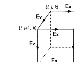
solution region including air is discretized into rectangular cells. The secondary electric field is de-fined at the center of the cell edges as shown in Fig. 1. The conductivity at each sampling point is repre-sented by a weighted average of conductivities of the four adjoining cells; the weights are proportional to the cross-sectional area of each cell that is normal to the sampled field component. As boundary
condi-Fig. 1. Sampling positions for the electric field components on a staggered grid.
tions, the tangential component of E is set equal tos
zero on the boundaries of the model. Approximating
Ž .
Eq. 6 with finite differences results in a linear system of equations,
K fss,
Ž .
8where K is a symmetric complex matrix, f is the unknown vector for the secondary electric field, and
s is a vector containing source terms. All elements of
Ž .
K are real except for the diagonal elements. Eq. 8
Ž .
can be solved using the biconjugate gradient BCG method, preconditioned with an incomplete Cholesky decomposition. The preconditioning schemes using standard incomplete Cholesky decompositions break down because K is not positive-definite. However,
Ž .
Mackie et al. 1994 shows that this difficulty can be avoided by applying the decomposition only to the diagonal subblocks that are positive-definite, when K is grouped into subblocks depending on the related components of the electric fields. Although reason-able convergence rates can be obtained with the
Ž .
incomplete Cholesky biconjugate gradient ICBCG method in many instances, they tend to be degraded as the frequency falls. This is because conservation of current is not guaranteed in a discretized version
Ž .
of Eq. 6 when the second term of the left-hand side
Ž .
4. Sensitivity
A common approach to derive the sensitivity is to
Ž
use the reciprocity of the Green’s functions Weidelt, 1975; Pellerin et al., 1993; Mackie and Madden,
.
1993 . If a 3-D conductivity structure is perturbed over a 3-D region, Õ, by an amount ds, then the
resulting magnetic field H at a receiving point r ist
given by
where H is the magnetic field for the unperturbed model and E is the electric field for the perturbedt
H Ž X.
model. The tensor Green’s function G r, r is the magnetic field at r for the unperturbed model, due to a unit electric dipole source at rX. Under the Born approximation, the perturbation of the magnetic field,
dH, is approximated by
dHf
H
GHŽ
r , rX.
PE rŽ .
X dsŽ .
rX dÕX,Ž
10.
Õ
where E is the electric field for the unperturbed model. Considering the components of the magnetic
Ž .
field, say, the x-component, Eq. 10 reduces to
dH s GH r , rX magnetic field at r, due to the y-directed unit elec-tric dipole source at rX. Using the reciprocity rela-tion,
Gi jH
Ž
r , rX.
sGjiHŽ
r , rX.
,Ž
12.
H Ž X.
we can interpret Gx y r, r as representing the y-component of the electric field at rX due to the x-directed magnetic dipole source placed at the re-ceiving point r. Replacing the magnetic Green’s
Ž .
function with the reciprocal electric field, Eq. 11 becomes
y1 X X X X
M x
dHxs
H
EŽ .
r PE rŽ .
dsŽ .
r dÕ,Ž
13.
ivm Õ
where EM x denotes the electric field due to the
x-directed magnetic dipole source with unit moment placed at the receiving point. If the region Õ
corre-sponds to the mth block and its conductivity is sm, we obtain
EHxs y1
H
EM xŽ .
rX PE r dŽ .
X ÕX.Ž
14.
Esm ivm Õ
The sensitivities of the other components of the EM fields are derived in the same way. For example, the sensitivity of the y-component of the electric field is given by
where EJ y denotes the electric field due to the
y-directed unit electric dipole source at the receiving
Ž . Ž .
point. Eqs. 14 and 15 show that the sensitivities can be obtained by doing forward modelings with the fictitious and actual sources and by integrating the dot product of the electric fields. Notice that the fictitious sources are placed at each receiving point instead of in each model block, which results in a significant saving in computation time. This proce-dure is referred to as the adjoint-equation method by
Ž .
McGillivray et al. 1994 .
Another approach to arrive at the above procedure
Ž .
is to begin with the matrix Eq. 8 . Differentiating
Ž .
Eq. 8 with respect to the block conductivity sm
yields
Ef EK
K s y f .
Ž
16.
Esm Esm
Ž .
By analogy with Eq. 8 , the derivative of the field with respect to sm can be interpreted as the field due to a collection of sources described by the right-hand
Ž .
side of Eq. 16 . This new source term is the product of the derivative of K and the column vector of the field for the model. The derivative of the element of
sources are present only in the block of interest. In the finite-difference approximation, the elements of
K that contain the conductivity are the diagonal
elements, and they have the form ivms DÕ, where
i i
s is the conductivity of an elemental volume DÕ
i i
Že.g., Newman and Alumbaugh, 1995 . Thus, the.
sources in the block have the strength of DÕ
multi-i plied by the electric field E . Using the reciprocity, iti turns out that the derivative of the field is equal to a weighted sum of the fields over the block due to a unit source placed at the receiving point, where the weights are given byDÕiE . This weighted summa-i
Ž .
tion amounts to the integration in Eq. 15 .
In the examples below, EM data are inverted for the logarithms of resistivities. The sensitivities are computed through the relation
Ef Ef
s ysm ,
Ž
17.
Elnrm Esm
Ž .
where rm is resistivity i.e., rms1rsm .
5. Verification of forward solution
In order to check the accuracy of the forward solution, it was compared with the finite-difference
Ž .
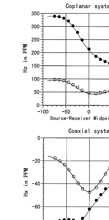
solution of Newman and Alumbaugh 1995 . Fig. 2 shows a model used to simulate airborne EM
re-Fig. 2. The 2-D model used in the forward modeling comparisons
Žafter Newman and Alumbaugh, 1995 ..
Fig. 3. Comparison between two finite-difference solutions. Shown are the magnetic field responses for the coplanar and coaxial systems. The open and closed circles represent the real and imaginary components, respectively, obtained in this study, while the solid lines represent the result from Newman and Alumbaugh
Ž1995 ..
sponses. A 2-D body of resistivity 1 V m is placed along a vertical fault contact. The resistivity left of the contact is 100 V m, while the resistivity right of the contact is 300 V m. The transmitter and receiver are separated by a fixed distance of 10 m, 20 m above the earth’s surface. The magnetic field
re-Ž .
sponses for both horizontal coil coplanar TzyRz
Ž .
and vertical coil coaxial TxyRx systems were
Ž .
Fig. 4. A plot of the squared residual versus iteration number using the ICBCG method with and without the divergence
correc-5 52 5 52 tion. The squared residual is defined as K fys r s .
between the two solutions are shown in Fig. 3, with good agreement for both source configurations. Fig. 4 shows a plot of the squared residual as a function of iteration number for the ICBCG method with and without the static divergence correction. It is evident that due to the divergence correction, the conver-gence of ICBCG iterations is significantly improved. The computer time required per source location was
Ž .
approximately 2 min on a Pentium II 450 MHz PC.
6. Synthetic data examples
In this section, two examples of 3-D inversion of noise-free synthetic data are presented. The first example simulates airborne EM surveys with two different coil configurations, and the second simu-lates a ground EM survey. The ‘observed’ data are generated with the finite-difference solution.
6.1. Airborne EM
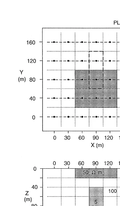
The model used to generate the data is shown in Fig. 5. It consists of a 50 V m surface body and a 5
V m buried body in a 100 V m background half-space. In the plan view of Fig. 5, the observation points are represented by the solid circles and the flight lines are represented by the heavy dashed lines. The flight lines are 20 m above the earth’s surface and the transmitter–receiver separation is 10
m. The frequencies used are 1, 4, and 8 kHz. Two
Ž .
data sets were generated for the coplanar TzyRz
Ž .
and coaxial TxyRx systems; the data are in the form of real and imaginary components of magnetic
Ž .
fields, and one data set consists of 210 real number data points.
In the inversion, the model was divided into 175
Žs7=5=5 blocks of unknown resistivity and for-.
ward modelings were performed using a grid of
Ž .
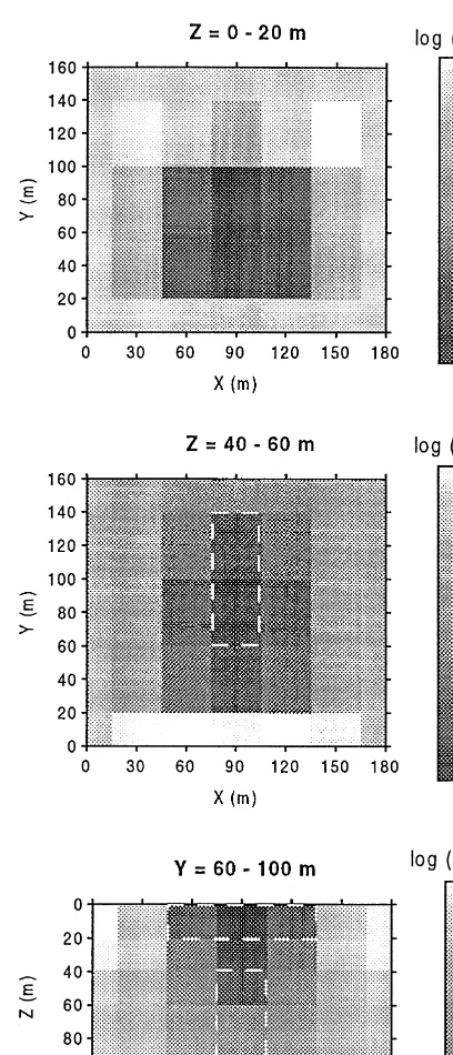
27,744 s34=34=24 cells. The initial model was a homogeneous half-space of 100 V m. The data were weighted with the reciprocal of their am-plitudes. The results of the inversion for the coplanar system are shown in Fig. 6. The upper panel is a horizontal slice at a depth of 0–20 m, the middle panel is a deeper horizontal slice at a depth of 40–60
Fig. 6. Reconstructed log resistivity for the inversion of the airborne EM data for the coplanar system.
m, and the lower panel is a vertical slice through the central flight line. The lateral extent of the surface body is clearly defined. Although the buried conduc-tor is obscured by the surface body, its lateral
loca-tion can be recognized. The reason for the poor resolution in the depth direction is that the data with three frequencies do not provide enough information to derive the detailed resistivity variations with depth. The inversion result for the coaxial system is shown
in Fig. 7. The buried conductor as well as the surface body are more clearly recovered. This is consistent
Ž .
with the observation by Liu and Becker 1990 that the resolution of the coaxial system along the survey line is better than that of the coplanar system. The convergence plots are shown in Fig. 8. The rms misfit at the third iteration is 0.6% and 0.7% for the coplanar and coaxial systems, respectively. The com-puter time needed for each inversion is approxi-mately 25 h on a Pentium II PC. The memory used was 39 Mb.
6.2. Ground EM
The model used to simulate a ground EM survey is shown in Fig. 9. Two 3-D bodies of 10 V m are embedded in a homogeneous background medium of 100 V m. The open circles in the plan view repre-sent the source points, which are also used as receiv-ing points. The sources are vertical magnetic dipole
ŽVMD , operating at frequencies of 2, 4, and 8 kHz..
For each source, the vertical magnetic fields were computed at the receiver points along the x- and y-directed lines passing through the source point. This yields a total of 48 transmitter–receiver combi-nations; hence the number of data points is 288. In
Ž
the inversion, the model was divided into 384 s8
.
=8=6 blocks of unknown resistivity and a grid of
Ž .
33,524 s34=34=29 cells was used in the for-ward modeling. The initial model was a
homoge-Fig. 8. Convergence plot for the inversions resulting in the models shown in Figs. 6 and 7.
Fig. 9. 3-D model used to generate ground EM data.
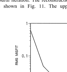
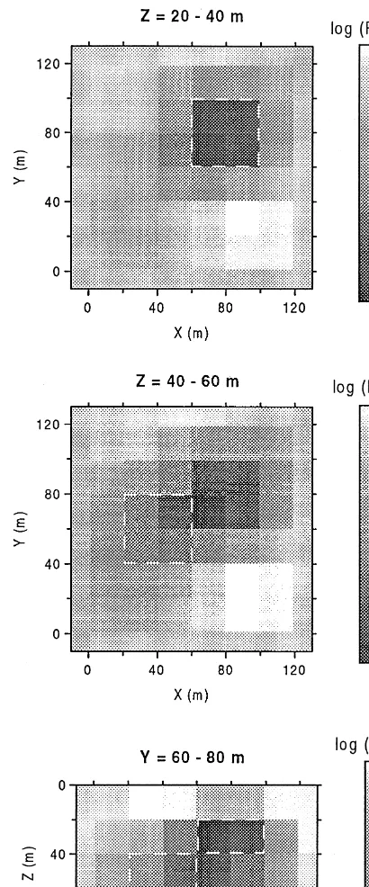
neous half-space of 100 V m. As shown in Fig. 10, a nearly 1% level of misfit was achieved at the fourth iteration. The reconstruction of the resistivity is shown in Fig. 11. The upper panel shows a
Fig. 11. Reconstructed log resistivity for the inversion of ground EM data.
horizontal slice at a depth of 20–40 m, the middle panel shows a deeper horizontal slice at a depth of
40–60 m, and the lower panel shows a vertical slice at Ys60–80 m. The shallower body is basically recovered, but the lower body is fairly blurred. One possible reason for this is that the survey coverage or the aperture is not wide enough to illuminate the deeper part of the model. Thus, one could obtain better resolution by expanding the survey coverage area. The time required to do this inversion was 12 h on a Pentium II PC, and the memory used was 56 Mb. This computer time is about one-half that spent in the previous example. This large difference in the computer time arises from the fact that in this exam-ple the source points are also used as the receiving points and hence very few additional forward model-ings are required to compute the sensitivities.
7. Conclusions
A method to invert controlled-source EM data for 3-D structure has been described. The forward calcu-lations are based on a staggered-grid finite difference scheme for the secondary electric field. The system of equations resulting from the finite-differencing is solved using the ICBCG method, and the conver-gence rates are improved by incorporating the static divergence correction. As a result the forward calcu-lation per source location takes only a few minutes on a PC. The sensitivities are obtained from the forward solutions using the reciprocity relation. The inverse problem is formulated so that a model is found that has a smooth structure and at the same time is close to an initial model, and is solved with an iterative least-squares method. The synthetic ex-amples show that 3-D inversions are feasible on PC and give reasonably accurate results for simple 3-D models. However, when considering the amount of data collected in field surveys, particularly in air-borne EM surveys, further work is required to make 3-D inversions more efficient.
Acknowledgements
References
Eaton, P.A., 1989. 3D electromagnetic inversion using integral equations. Geophys. Prosp. 37, 407–426.
Ellis, R.G., 1995. Joint 3D EM inversion. Symposium on Three-Dimensional Electromagnetics, Proceedings, Schlumberger-Doll Research, Ridgefield, Connecticut. pp. 307–323. Lines, L.R., Treitel, S., 1984. Tutorial: a review of least-squares
inversion and its application to geophysical problems. Geo-phys. Prosp. 32, 159–186.
Liu, G., Becker, A., 1990. Two-dimensional mapping of sea-ice keels with airborne electromagnetics. Geophysics 55, 239–248. Mackie, R.L., Madden, T.R., 1993. Three-dimensional magne-totelluric inversion using conjugate gradients. Geophys. J. Int. 115, 215–229.
Mackie, R.L., Smith, J.T., Madden, T.R., 1994. Three-dimen-sional electromagnetic modeling using finite difference equa-tions: the magnetotelluric example. Radio Sci. 29, 923–935. McGillivray, P.R., Oldenburg, D.W., Ellis, R.G., Habashy, T.M.,
1994. Calculation of sensitivities for the frequency-domain electromagnetic problem. Geophys. J. Int. 116, 1–4. Newman, G.A., 1995. Crosswell electromagnetic inversion using
integral and differential equations. Geophysics 60, 899–911.
Newman, G.A., Alumbaugh, D.L., 1995. Frequency-domain mod-eling of airborne electromagnetic responses using staggered finite differences. Geophys. Prosp. 43, 1021–1042.
Newman, G.A., Alumbaugh, D.L., 1997. Three-dimensional mas-sively parallel electromagnetic inversion: I. Theory. Geophys. J. Int. 128, 345–354.
Oldenburg, D.W., McGillivray, P.R., Ellis, R.G., 1993. General-ized subspace methods for large-scale inverse problems. Geo-phys. J. Int. 114, 12–20.
Pellerin, L., Johnston, J.M., Hohmann, G.W., 1993. Three-dimen-sional inversion of electromagnetic data. Expanded Abstracts, 63rd SEG Annual International Meeting, Washington, D.C. pp. 360–363.
Smith, J.T., 1996. Conservative modeling of 3-D electromagnetic fields: Part II. Biconjugate gradient solution and an accelera-tor. Geophysics 61, 1319–1324.
Weidelt, P., 1975. Inversion of two-dimensional conductivity structures. Phys. Earth Planet Inter. 10, 282–291.