www.elsevier.nlrlocaterjappgeo
Dielectric constant determination using ground-penetrating radar
reflection coefficients
Philip M. Reppert
), F. Dale Morgan, M. Nafi Toksoz
¨
Earth Resources Laboratory, Department of Earth, Atmospheric, and Planetary Sciences, Massachusetts Institute of Technology, Cambridge, MA 02142, USA
Received 14 September 1998; received in revised form 22 February 1999; accepted 21 May 1999
Abstract
Ž .
A method to determine ground-penetrating radar GPR velocities, which utilize Brewster angles, is presented. The method determines the relative dielectric constant ratio at interface boundaries where the radar wave is traveling from a low-velocity to a high-velocity medium. Using Brewster angle analysis is currently the only means to determine the velocity of the medium below the deepest detectable reflector. Data are presented for water-saturated clean sand with a known velocity of 0.52 mrns, which overlays a sandy silt with a known velocity of 0.13 mrns. Brewster angle analysis of a
Ž .
common midpoint CMP survey gives a relative dielectric constant ratio of 33r4.77. The Brewster angle relative dielectric constant ratio is in good agreement with the relative dielectric constant ratio calculated from the known velocities.q2000
Elsevier Science B.V. All rights reserved.
Keywords: Brewster angle; Dielectric constant; Radar; GPR; Velocity
1. Introduction
Ž .
Ground-penetrating radar GPR has gained popularity in recent years owing to its speed and ease of use. Two of its primary uses are anomaly
Ž .
detection and electromagnetic EM velocity de-termination of the shallow subsurface. Velocity analysis has been limited to common midpoint
ŽCMP surveys, which give the velocity struc-.
ture above a reflector at a single location. This study presents and demonstrates a method that
)Corresponding author. E-mail: [email protected]
uses Brewster angles for determining the veloc-ity directly below the deepest detectable reflec-tor.
Knowing the EM velocity structure of the shallow subsurface is important in identifying electrical properties of different reflectors. The electrical properties are related to the composi-tion of the reflectors. Sometimes, a situacomposi-tion is encountered when a low-velocity layer is lo-cated above a high-velocity layer, where no reflections can be obtained below the high-velocity layer. Consequently, the high-velocity of the high-velocity layer cannot be obtained using traditional techniques. The remainder of this paper will describe the theory for determining
0926-9851r00r$ - see front matterq2000 Elsevier Science B.V. All rights reserved.
Ž .
the velocity of the high-velocity layer and demonstrate its effectiveness with an example.
2. Background
GPR is most frequently used to perform re-flection profiles, which are commonly referred to as zero offset profiles. Such profiles are acquired by keeping the two GPR antennas an equal distance apart while taking measurements
Ž
at equal spacing along a traverse Davis and
.
Annan, 1989 . When viewing a zero offset pro-file, one is often looking at the topography of a layer or for anomalies in the reflection signal, such as hyperbolas associated with small buried objects. Due to the interpretation non-unique-ness of radar images, errors may occur in inter-preting the source of the buried layer or anomaly. Is the hyperbola caused by a buried barrel or by a boulder? If one is looking at a horizontal reflector, how does one determine whether the anomaly is a water-table boundary or clay-layer boundary? The difficulty in interpreting GPR data is due to many factors such as attenuation, dispersion, scattering and radiation patterns
ŽAnnan, 1996 . Using travel time analysis in.
conjunction with a zero offset profile can reduce some of the problems associated with these factors.
Velocity travel-time analysis used in conjunc-tion with the CMP data acquisiconjunc-tion method is the traditional technique for determining the
Ž
composition of a reflector Annan and Cosway,
.
1992 . However, there are limitations associated with this method. To use this technique, one must look at radar wave velocities using travel times for the reflected waves. Consequently, the velocity of the medium below the lowest reflec-tor cannot be determined.
3. Theory
The theoretical basis for GPR is found in Maxwell’s equations. However, it is not the
intent of this paper to provide an in-depth math-ematical derivation of the EM wave equation from Maxwell’s equations. For more detailed information on the derivation, Keller and
Zh-Ž . Ž .
danov 1994 and Wait 1982 contain thorough discussions of the subject. The success of GPR is based on EM waves operating in the frequency range where displacement currents dominate and losses associated with conduction
Ž .
currents are minimal Annan, 1996 . For the purposes of this paper, the assumption is made that we are dealing only with displacement cur-rents and that the medium is lossless. The justi-fication for this assumption will be discussed later.
The wave equation, in the propagation regime for electric displacement currents, is given in
Ž .
where E is the electric field, m is the magnetic permeability and ´ is the permittivity. The per-mittivity can be defined as ´s´ ´o r, where ´o
is the permittivity of free space and ´r is the relative dielectric constant. Using phasor
nota-Ž .
tion, Eq. 1 can be represented as shown in Eq.
Ž .2 , where v is the angular frequency:
=2Es yv2m´E.
Ž .
2The velocity for an EM wave in a dielectric is given by:
where s represents conductivity. At high
fre-Ž .
quencies andror very low conductivity, Eq. 3 reduces to:
1
ys .
Ž .
4(
m´medium. For insulating materials such as dry rocks, dielectric properties alone determine the velocity of the EM wave. The effect that dielec-tric properties can have is seen in Figs. 1 and 2. Fig. 1 plots the velocity of an EM wave as a function of conductivity and frequency with a relative dielectric constant of 4. It can be seen in Fig. 1 that for frequencies greater than 100
Ž .
MHz, Eq. 4 is a good approximation of the velocity. For frequencies below 100 MHz, the
Ž .
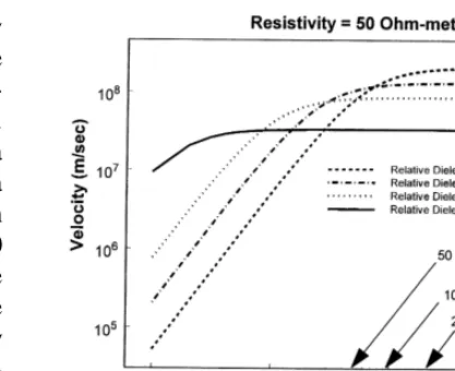
use of Eq. 4 will depend on the conductivity of the medium. Fig. 2 plots frequency vs. rela-tive dielectric constant with a constant resistiv-ity of 50 V m. It can be determined from Fig. 2
Ž .
and Eq. 4 that for frequencies above 100 MHz, velocity is essentially independent of fre-quency and dependent only on the dielectric constant and the magnetic permeability.
Earth materials rarely have a magnetic per-meability appreciably different from unity
ex-Ž .
cept for a few magnetic minerals see Table 1 . Magnetic permeability generally has a notice-able effect only when large quantities of Fe O2 3
Ž .
are present Telford et al., 1990 . Therefore, changes in velocity must be due to changes in dielectric constant or changes in resistivity of the medium. Consequently, for many earth ma-terials, at high frequencies or high resistivity,
Fig. 1. Velocity of an EM wave plotted as a function of the soil resistivity with a relative dielectric constant of 4.
Fig. 2. Velocity of an EM wave plotted as a function of the relative dielectric constant with a resistivity of 50 V m.
the velocity of an EM wave is determined only by the relative dielectric constant of the medium. Table 2 gives a list of relative dielectric con-stants and conductivities for a variety of earth materials encountered when using GPR.
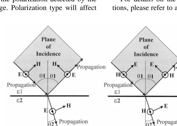
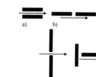
When EM waves are obliquely incident on an interface between two media, it is necessary to consider two different cases. The first case ex-ists when the electric field vector is perpendicu-lar to the plane of incidence. This is commonly referred to as perpendicular polarization. The plane of incidence is the plane containing the incident ray and is normal to the surface. The second case exists when the electric field vector is parallel to the plane of incidence. This case is commonly referred to as parallel polarization. For schematic representations of these two cases, refer to Fig. 3a and b.
Table 1
List of relative magnetic permeabilities of various minerals
Žadapted from Telford et al., 1990.
Mineral Permeability
Magnetite 5
Pyrrhotite 2.55
Hematite 1.05
Rutile 1.0000035
Calcite 0.999987
Table 2
List of relative dielectric constants and velocities for some
Ž
typical earth materials adapted from Annan and Cosway,
.
1992
Ž .
Material Relative dielectric Velocity mrns constant
Air 1 0.30
Sea water 80 0.01
Dry sand 3–5 0.15
Saturated sand 20–30 0.06
Limestone 4–8 0.12
Silts 5–30 0.07
Granite 4–6 0.13
Ice 3–4 0.16
EM waves may become polarized when radi-ated from an antenna. The antenna design deter-mines the type of polarization, which can be linear, circular, or elliptical. Most GPR antennas emit waves that are linearly polarized, which are further subdivided into perpendicular or par-allel polarized. By changing the orientation of the antennas relative to each other and relative to the traverse, the polarization detected by the radar will change. Polarization type will affect
how the wave is reflected from a planar surface or a buried object. The reflection differences show up in the reflection coefficients of the two cases. For a thorough discussion on the subject of polarization of radar waves, refer to Roberts
Ž .
and Daniels 1996 .
The perpendicular polarized reflection coeffi-cient equation is:
2
(
´ cosu y ´ y´ sin u Er
(
1 1 2 1 1s ,
Ž .
52
Ei
(
´1 cosu1q(
´2y´1sin u1and the parallel polarized reflection coefficient
Ž .
equation, Eq. 6 , gives the ratio of reflected signal to incident signal at a horizontal planar boundary:
´2 ´2 2
cosu1y
)
ysin u1ž /
´ž /
´Er 1 1
s .
Ž .
6Ei ´2 ´2
2
cosu1q
)
ysin u1ž /
´1ž /
´1For details on the derivation of these equa-tions, please refer to any textbook on EM theory
Ž .
Fig. 3. Schematic diagram of perpendicular and parallel polarized EM waves. a shows a perpendicular polarized EM wave where the E field points out of the page perpendicular to the plane of incidence and the H field is parallel to the plane of
Ž .
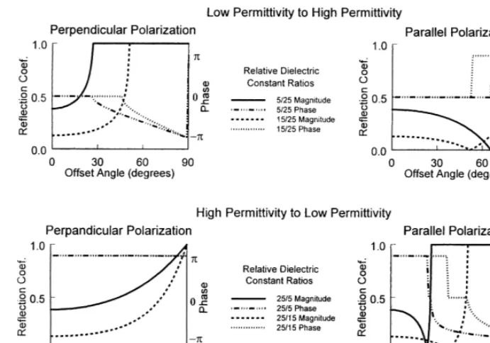
Fig. 4. Magnitude and phase portion of reflection coefficients for two different velocity contrasts. Parallel and perpendicular polarizations are shown when the EM wave goes from low velocity to high velocity and from high velocity to low velocity.
such as Electromagnetic Waves and Radiating
Ž .
Systems Jordan and Balmain, 1968 . Plots of the reflection coefficients vs. angle of incidence for both the parallel and perpendicular polarized waves are shown in Fig. 4. This figure shows the magnitude and phase portion of the reflec-tion coefficients.
For parallel polarized waves, there exists an angle where no reflected wave exists. This an-gle is referred to as the Brewster anan-gle and
Ž .
given by Eq. 7 . The Brewster angle occurs
Ž .
when the numerator in Eq. 6 goes to zero:
´2
tanu1s
(
.Ž .
7´1
The Brewster angle is more easily understood when one looks at the magnitude and phase portions of Fig. 4. The Brewster angle occurs in Fig. 4b and d when a step change of 908 in phase occurs prior to reaching the critical angle where all energies are reflected from the inter-face. When a step change of 908in phase occurs prior to all energies being reflected, the
re-flected energy goes to zero. When viewing Fig. 4c and d, other phase changes are evident and these occur after all energies have been re-flected. It should be noted that these phase changes are not step changes in phase.
4. Application of theory
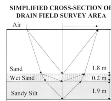
Fig. 5. Simplified cross-section of the drain field survey area.
location of the phase change is found, the Brew-ster angle position can be determined from the radar plot. The depth of the reflector can be determined using traditional velocity analysis. Once the depth of the reflector is determined, the Brewster angle can be calculated and a relative reflection coefficient can be determined.
Ž
Because the velocity relative dielectric
con-.
stant can be determined for the medium above the reflector, the relative dielectric constant and velocity can be determined for the medium below the reflector using the Brewster angle and
Ž .
Eq. 7 .
5. Data collection
A field study was conducted to test whether the Brewster angle could be detected and used to determine relative dielectric constants and velocities. Data were collected over a recently constructed drain field in Ashby, MA. Bedrock in the area consists of a light gray, medium-grained, weakly foliated, weakly metamor-phosed granite that is of the Fitchburg Complex. The overburden of the drain field consists of clean sand overlying sandy silt, which contains various-sized cobbles which overlie the hard-pan. Hardpan is a term used to refer to glacial till that has been compacted to the point where pneumatic hammers are required to excavate the material.
The drain field data consist of the layers that are shown in Fig. 5. These layers are: Layer 1, air; Layer 2, 1.8 m of clean sand; Layer 3, 0.2 m of water-saturated clean sand; Layer 4, 1.9 m of sandy silt; Layer 5, hardpan. Initial drain field stratification data were obtained from a deep-hole survey conducted prior to the con-struction of the drain field. Radar calculation of the depths of the strata is in agreement with the deep hole data except for the location of the water saturation zone. However, the water satu-ration zone moved due to seasonal fluctuations in the water table.
The data were collected using a Pulse Ekko IV radar with 200 MHz antennas. A reflection profile of the survey line, using a perpendicular broadside antenna configuration, is shown in Fig. 6 with the center point of the CMP located 2 m on the reflection profile. The CMP is shown in Fig. 7 with the events of interest
Ž . Ž .
marked. Event a is the air wave, b is the
Ž .
ground wave, c is the reflection from the top
Ž .
of the water-saturated sand, d is the bottom of the water-saturated sand and the top of the
Ž .
sandy silt, and e is the top of the hardpand. The CMP was performed using the parallel endfire antenna configuration. The parallel end-fire configuration is shown in Fig. 8 along with other antenna configurations.
Traditional X2–T2 velocity analysis was
done on the CMP data, giving the air velocity as 0.3 mrns. The average velocity of the sand, Layer 2, is approximately 0.114 mrns. The average velocity of the water-saturated sand is approximately 0.052 mrns and the velocity of the sandy silt is 0.13 mrns. A velocity profile is shown in Fig. 6 along with the reflection pro-file.
Based on the discussions in Section 3, the Brewster angle will be found on the interface
Fig. 7. CMP raw data of the test site. The data were collected with a 200 MHz pulse EKKO IV system. Event
Ž .a is the air wave, b is the ground wave, c is theŽ . Ž . Ž .
reflection from the top of the water saturated sand, d is the bottom of the water-saturated sand and the top the
Ž .
sandy silt, e is the top of the hardpand which is also referred to as compacted glacial till.
Ž .
Fig. 8. GPR antenna configurations, a parallel broadside,
Ž .b parallel endfire, c perpendicular broadside, d per-Ž . Ž . Ž .
pendicular endfire, e cross-polarization.
that is bounded by a low-velocity layer above the interface and a high-velocity layer below the interface. Therefore, from the previous velocity analysis, the Brewster angle should be found on the event made by the interface between the water-saturated sand and the sandy silt, event
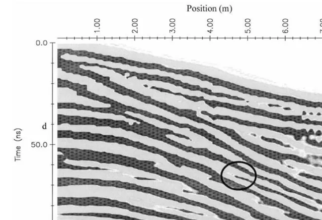
Ž .d shown in Fig. 7. Following event d in Fig.Ž .
9, which starts at approximately 42 ns, a phase change can be seen at approximately 4.5 m. Using travel time curves constructed from the traditional velocity analysis, the incident angle for each offset distance is calculated for event
Ž .d . A horizontal distance of 4.5 m gives an angle of 20.778 for the incident ray contacting the interface. A relative dielectric constant of 33 for the water-saturated clean sand was deter-mined using the X2–T2 velocity of 0.052 mrns. Using this relative dielectric constant, the angle determined above, and the Brewster angle
equa-Ž .
tion, Eq. 7 , a relative dielectric constant of 4.78 was calculated for the sandy silt. In turn, a relative dielectric constant of 4.78 gives a veloc-ity of 0.1369 mrns, which is comparable to a velocity of 0.13 mrns that was determined using traditional X2–T2 velocity analysis.
Comparisons of the velocities determined using
X2–T2 analysis and the Brewster angle method are given in Table 3.
Fig. 9. Color plot of the data shown in Fig. 7. The Brewster angle location is highlighted by the circled area.
Ž .
reflection coefficient, calculated from Eq. 6 , was converted to amplitudes by multiplying the theoretical reflection coefficients by a constant. The same equation was used to generate the model for Fig. 4 where a parallel polarized wave goes from high permittivity to low permit-tivity. A simple exponential attenuation was then applied to the theoretical amplitudes. As can be seen in Fig. 10, there is good similarity
Ž .
between the data amplitudes from event d and the theoretical amplitudes. It can also be seen in Fig. 10 that two changes in phase occur for this relative dielectric constant ratio, one at 20.778
Table 3
Comparison of velocities determined using X2– T2
analy-sis and Brewster angle analyanaly-sis
2 2
Layer Material Brewster angle X – T
Ž .
velocity mrns velocity
Žmrns.
1 air 0.3
2 clean sand 0.114
3 water-saturated sand 0.052
4 sandy silt 0.137 0.13
5 hardpan 0.153–0.17
and the other at 23.758. An incident angle of
Ž .
23.758 on event d gives a surface distance of approximately 7.25 m. When the event is exam-ined, another phase change is apparent at 7.25 m. On first examination, it seems unusual that a small change in angle of the incident ray, 38,
Fig. 10. Real portion of theoretical amplitudes for a rela-tive dielectric constant ratio of 33r4.8. The Brewster angle occurs at 20.778. The amplitudes were obtained by multi-plying the reflection coefficients by a constant and then multiplying by a simple exponential attenuation. The
the-Ž .
should occur over such a large surface offset, 2.5 m, when the depth of the reflector is only 2 m deep. However, due to the phenomenon of ray bending at interface boundaries, small changes in incident angle can occur with large surface offset distances.
For completeness, there are other anomalies in Fig. 9, which must be addressed. At position 2 m and 18 ns, 3.8 m and 30 ns, and 6 m and 45 ns, these anomalies resemble some time of phase change. It is apparent from the plot that these anomalies are caused by the critically refracted air wave. This conclusion can be confirmed by the slope of the events as well as by construct-ing travel time curves. The anomalies at posi-tions 2 m and 30 ns and 3 m and 40 ns are caused by the first reflector merging into the
Ž .
direct wave ground wave . Again, this can be confirmed by construction of travel time curves. It should also be noted that none of the above anomalies has the same characteristics as the anomaly identified as the Brewster angle.
Ž .
Below event d , it is not possible to deter-mine velocities to use to confirm any value determined using the Brewster angle method. Positions 1 m and 2 m at 60 ns appear to be weak reflectors. This conclusion was arrived at by looking at the wave forms and amplitudes of individual events. From the velocity analysis
Ž .
and the deep hole data, event e is on the interface of the sandy silt and hardpan. At the
Ž .
positions of 2.4 m and 4.2 m on event e , the anomaly appears to be similar to the Brewster
Ž .
angle on event d . Using the same type of analysis as above, angles of 418 and 548 for the first and second phase change, respectively, are obtained. These angles do not give a perfect fit to a reflection coefficient curve but are within expected measurement errors. They give a range of relative dielectric constant ratios for the sandy siltrhardpan interface of 4.77r3.4 to 4.77r3, which gives a range of velocities of 0.153–0.17 mrns for the hardpan. The first velocity is not unrealistic based on the velocity of the sandy silt, but this velocity cannot be substantiated at the present time.
6. Summary
Brewster angles can be used to determine relative dielectric constants and velocities. Pre-liminary results appear to support the theory. This method has the advantage of being useful in determining the velocity of the medium be-low the deepest detectable reflector. The use of Brewster angles is restricted to horizontal planar targets compared to the wavelength of the an-tenna. If the dipping angle of planar target is known, it may be possible to use this method on nonhorizontal targets. Also, this method is lim-ited by the velocity contrasts in the subsurface. Certain combinations of velocity contrasts may prevent the Brewster angle from being reached before the GPR signal is lost. Future work in the area will include the construction of a test pit to better understand Brewster angle reflec-tions in a variety of controlled condireflec-tions.
Acknowledgements
We thank David Cist for his insightful dis-cussions regarding this project. We especially thank Chantal Mattei and Nancy Reppert for their assistance in collecting the radar data.
References
Annan, A.P., 1996. Transmission dispersion and GPR. JEEG 0:2, 125–136.
Annan, A.P., Cosway, S.W., 1992. Ground-penetrating radar survey design. Paper prepared for Annual Meet-ing of SAGEEP.
Davis, J.L., Annan, A.P., 1989. Ground-penetrating radar for high-resolution mapping of soil and rock stratigra-phy. Geophysical Prospecting 37, 531–551.
Jordan, E.C., Balmain, K.G., 1968. Electromagnetic Waves and Radiating Systems. Prentice-Hall, NJ, pp. 139–144. Keller, G.V., Zhdanov, M.S., 1994. The Geoelectrical Methods in Geophysical Exploration. Elsevier, Amster-dam.
Roberts, R.L., Daniels, J.J., 1996. Analysis of GPR
polar-Ž .
ization phenomena. JEEG 1 2 , 139–157.
Telford, W.M., Geldart, L.P., Sheriff, R.E., 1990. Applied Geophysics. Cambridge Univ. Press, MA, p. 291. Wait, J.R., 1982. Geo-Electromagnetism. Academic Press,