Suitable Policy Instruments for
Monetary Rules
Saranna R. Thornton
The performance of different policy instruments is examined in counterfactual simulations using McCallum’s adaptive rule. Three different macroeconomic models are used, re-spectively, to simulate values of nominal GDP from 1964:Q1–1995:Q4.
In comparison with historical, discretionary monetary policy, rules using M2 as the policy instrument produce substantial reductions in the variability of GDP around a fixed trend—even with money control error. M2 performs well, despite the presence of money control error, because the feedback term in McCallum’s rule, in combination with the relative stability of the linkage between M2 and GDP, successfully counteracts most of the impacts of undesired quarterly changes in money growth. © 1998 Elsevier Science Inc.
Keywords: Monetary policy; Monetary rule
JEL classification: E42, E52
I. Introduction
The introduction of bills in Congress that mandate price stability as the Fed’s primary policy objective, and the support these bills received from Federal Reserve Officials and other economists, suggests a growing consensus on the primary goal of monetary policy. Yet, debate continues regarding the appropriate means, to achieve this goal. Some propose using discretionary monetary policy, while others favor monetary rules.
Supporters of rules argue that discretionary policy will exhibit an inflationary bias when the central bank’s objective function negatively weights inflation and positively weights levels of output above the full-employment level.1Proponents of rules argue that inflationary bias can be eliminated if the central bank adopts a policy rule capable of
Department of Economics, Hampden-Sydney College, Hampden-Sydney, Virginia.
Address correspondence to: Dr. S. R. Thornton, Department of Economics, Hampden-Sydney College, Hampden-Sydney, VA 23943.
1Recent conduct of monetary policy does not contradict theory. Discretionary policy has been successful in
achieving inflation stability—not price stability. Furthermore, recent inflation stability is serendipitous and not invariant to the composition of the FOMC.
Journal of Economics and Business 1998; 50:379 –397 0148-6195 / 98 / $19.00
ensuring long-run price stability. Even central bankers acknowledge that policy rules can provide information useful in the formulation of discretionary policy.2
Interest in adaptive monetary rules has risen3as economists search for a rule that: 1) is operational; 2) performs well (i.e., ensures long-run price stability) in a variety of plausible macroeconomic models; 3) performs well when financial innovations or other shocks alter the linkages between the policy instrument and the intermediate target (e.g., velocity), and 4) promotes greater levels of price stability than historical discretionary policies have. In an attempt to isolate a rule that best meets these criteria, the performance of three versions of McCallum’s adaptive rule was evaluated from 1964:Q1–1995:Q4. Rules utilize M2, the St. Louis and the Federal Reserve Board Monetary Base, respec-tively, as policy instruments.4Rules utilizing M2 and the base were examined because research by McCallum (1987, 1988, 1990), Judd and Motley (1991, 1992), Feldstein and Stock (1993), Thornton (1993), among others, suggests these aggregates may meet the four key criteria listed above.
The performance of rules utilizing other commonly proposed policy instruments was not examined because research indicates that they don’t meet all criteria listed above. For example, Friedman (1988) found that rules utilizing measures of reserves are unlikely to ensure long-run price stability. Thornton (1993) found that M1 did not perform as well as M2 or the St. Louis monetary base in variations of McCallum’s rule. Judd and Motley (1992) found that interest rates did not perform well as a policy instrument in a rule which targeted a stable price level, and Clark (1994) found that a rule utilizing interest rates to target a stable inflation rate failed to reduce the variability of real GDP growth or inflation.5.
Section II reviews some issues regarding the choice of policy instrument and concludes that both M2 and the monetary base exhibit some deficiencies. Section III explains the GDP simulation procedure utilized to evaluate rule performance and develops baseline performance measures utilizing a St. Louis monetary base rule, a Federal Reserve Board monetary base rule, and an M2 rule6—the latter under an initial assumption of no money control error. Different measures of the base were used in order to consider the hypothesis that specification of the monetary base affects rule performance. Results were also derived utilizing an M2 rule which incorporates likely degrees of money control error. The performance of the policy rules is compared to assess their effectiveness. Section IV
2Statement by Governor Lawrence Meyer, January 5, 1997, AEA meetings, New Orleans, LA.
3See, for example, McCallum (1987, 1988, 1990); Judd and Motley (1991, 1992, 1993); Feldstein and Stock
(1993); Dotsey and Otrok (1994); Thornton (1993).
4M2 doesn’t meet the strict definition of a policy instrument as a variable under the direct control of the Fed.
M2 is considered an instrument for achieving a nominal income target, assuming there is an intermediate policy instrument utilized to target M2.
5The performance of interest rate rules in Clark (1994) may seem inconsistent with the Fed’s recent
experience using the Federal Funds rate to target a constant inflation rate. The inconsistency may be due to the specification of interest-rate rules. They typically include one feedback term which alters the policy instrument in response to a deviation from the rule’s nominal income target. In contrast, McCallum’s rule includes a velocity moving average term along with the feedback term. Both terms alter the policy instrument when the velocity growth rate (i.e., the linkage between the policy instrument and the target variable) changes. Proposed interest-rate rules can be thought of as analogous to McCallum’s rule, minus the velocity term. (And, in fact, in GDP simulations, McCallum’s rule did not perform as well, with only the feedback term.) Better results might be obtained with interest-rate rules by rewriting them to incorporate a term which explicitly adjusts the interest-rate response when there is a change in the relationship linking interest rates to income growth.
6All simulations utilize rules that target nominal income. Henceforth, the term ‘M2 rule’ or ‘monetary base
reviews some caveats bearing on any final determination of the success of a particular rule.
Results suggest that monetary base rules do not consistently produce greater levels of price stability—performance is model dependent. In contrast, the M2 rule consistently met the four criteria listed above during the sample period 1964:Q1–1995:Q4.
II. Choosing a Policy Instrument
Two operational concerns arise if the policy instrument is not directly and/or accurately controllable by the Fed. First, according to McCallum (1988), for a rule to be operational, there must be a way to monitor compliance. Because data on the components of the monetary base are available to Fed staff daily, the Fed can maintain more precise short-run control over the base than M2. The public can more easily monitor Fed compliance with base rules because money control error is unlikely to be a source of missed monetary base targets.7
Although short-run M2 control is less precise, compliance with an M2 rule might be gauged by establishing a narrow error band for the specified, quarterly M2 target level, as is commonly done with bilateral exchange rates under fixed exchange-rate regimes. Levels of M2 could be allowed to deviate from any given quarter’s target by the absolute value of a pre-specified, small percentage. Or, compliance could be measured by requiring the Fed to limit deviations from rule-specified M2 growth (measured in quarterly loga-rithmic units) to be zero on average with a mandated, relatively narrow variance.8The specified compliance period could be a longer period of time (e.g., one year). The size of the error band in the first measure of compliance or the variance and compliance period in the second measure must be large enough to accommodate the normal range of money control error, but small enough to prevent discretionary policy-making.
A second operational issue which arises from using M2 is that deviations of money growth from the quarterly, rule-specified targets may generate substantially greater deviations of nominal GDP from its target path. However, this problem might be mitigated in two ways. If money control errors exhibit a systematic, negative, contemporaneous correlation with GDP shocks, an M2 rule might not produce large deviations of simulated GDP from the target path. Alternatively, deviations of GDP from the target that are likely to result from the presence of money control errors may be small—if the impacts of the money control errors are mitigated by the rule’s feedback properties.
Feldstein and Stock (1993) noted that another important condition affecting the performance of a policy instrument is the existence of a sufficiently strong and stable relationship to nominal income. Although absolute stability in velocity growth is not a necessary condition for McCallum’s rule to be successful, the more stable the relationship between a policy instrument and GDP, the greater the degree of price stability. Although there are thresholds of instability which rule out the use of particular policy instruments,
7The monetary base is assumed to be controllable by the Fed over periods of time as short as one quarter.
This assumption is arguable because the Fed doesn’t perfectly control all of the items in its balance sheet. However, the Fed can control Federal Reserve Bank Credit (FRBC), the major item affecting the supply of reserves. Control of FRBC, combined with timely information on the most recent values of other items in the balance sheet and Fed staff forecasts of daily values of these other variables, should allow the Fed to maintain close, albeit imperfect, control of the monetary base over short time periods.
such large degrees of instability would also hamper the formulation of discretionary policy.
The strength and stability of the relationship between some policy instruments and income has been extensively examined. Friedman (1988) suggested that the relationship between the monetary base and nominal GNP has weakened as a result of surges in the growth rate of unusual types of currency demand (e.g., foreigners living in unstable economies, drug traffickers, etc.). More recent studies in the literature on money-income causality have utilized Granger causality tests to determine if interest rates, the monetary base or M2 exhibits significant predictive power for either nominal or real income. These studies have often yielded conflicting results because test outcomes were highly sensitive to the variables included, lag length, sample period, temporal aggregation of the data, and the use of vector autoregression (VAR) versus vector error correction models (VECM) for estimation of Granger-equations. Recent studies include Friedman and Kuttner (1992), Becketti and Morris (1992), Feldstein and Stock (1993), Abate and Boldin (1993), and Dotsey and Otrok (1994). With the exception of Friedman and Kuttner, these authors generally have found significant predictive power for M2 in equations modeling nominal or real income. Feldstein and Stock (1993) found that: 1) M2 is a useful predictor of nominal GDP; 2) the coefficients linking M2 to GDP appear to be stable over time; 3) M2 has more predictive content for nominal GDP growth than interest rates do, and 4) the relationship between the monetary base and nominal GDP appears to be highly unstable. The presence of various deficiencies in the policy instruments has caused questions regarding instrument efficacy to be addressed empirically by comparing rule performance in simulations utilizing different policy instruments in a variety of plausible macro models. Judd and Motley (1991, 1992), McCallum (1987, 1988, 1990), and Thornton (1993) found that monetary base rules can be used successfully to target nominal income. This result is robust for different time periods, different economic models, different start-up conditions, and the Lucas Critique. However, Friedman (1988) argued favorable results for the monetary base were a statistical artifact, based on the strong relationship between currency and GDP, rather than the relationship between the total reserves component of the base and GDP.
Results regarding M2 are mixed. Feldstein and Stock (1993) developed an M2 rule from a simple VAR model and found that the rule would probably reduce the average ten-year standard deviation of annual GDP growth by over 20%, thus reducing the long-run average inflation rate (assuming no M2 money control error). Thornton (1993) found that between 1964 and 1989, an M2 version of McCallum’s rule didn’t deliver substantially different levels of success in attaining the GNP target than a monetary base rule. This result was robust for different economic models, but simulations were con-ducted assuming no money control error. In contrast, Dotsey and Otrok (1994) found that the rule specified by Feldstein and Stock (1993) reduced the variance of nominal GDP only marginally (and not in all cases) when M2 money control errors were included in GDP simulations.
III. Evaluating the Performance of Monetary Base and M2 Rules
Recent research on rules which target nominal income has examined likely macroeco-nomic outcomes in cases where targets are specified in terms of either levels or growth rates. McCallum (1987, 1988, and 1990) defined the ultimate goal in terms of a constant, long-run, price level. But, McCallum (1993) changed the ultimate goal to zero inflation. Others, such as Fair and Howrey (1994), have specified the ultimate goal as a constant inflation rate roughly equal to a recent historical average.Specification of the ultimate goal depends on several factors, including the relative benefits of a constant price level or a stable inflation rate and the costs of disinflation.9 Rules examined here specify the nominal GDP target in levels, on the assumption that price stability is preferable to inflation stability. In order to assess the relative performance of the monetary base and M2, these policy instruments were used in variations of McCallum’s Rule (below) to simulate growth paths of nominal GDP in three macro models.
DRMt50.007392~1/16!~Xt212Xt2172Mt211Mt217!1l~X*t212Xt21!. (1)
where M is the log of the respective policy instrument (e.g., M2); 0.00739 is a 3% annual growth rate expressed in quarterly logarithmic units; X is the log of nominal GDP; X* is McCallum’s non-inflationary target path value of nominal GDP (i.e., a 3% growth path); lis a partial adjustment coefficient,10 and t indexes quarters. The rule-specified change in the money supply isDRM, and in cases where there is no money control error,DRM5 DM, the value of money growth that enters into the models of GDP determination. The second term on the right side of equation (1) is a four-year moving average growth rate of monetary velocity. The third term is a feedback adjustment that is activated when values of nominal GDP deviate from the non-inflationary target path.
Although parsimonious, the macroeconomic models utilized represent different, but not improbable, relationships between money and income. Although the models are open to econometric criticism, this doesn’t negate the utility of these simple models in the GDP simulations. As McCallum (1988) noted, model estimation produces parameter values which: 1) represent alternative theories of economic behavior, and 2) are consistent with actual U.S. economic data generated during the sample. The residuals computed in the course of model estimation were recycled in the GDP simulations as estimates of the actual shocks to the respective dependent variables being simulated.
Different macroeconomic models were utilized because a lack of consensus regarding the true economic model requires that conclusions regarding rules should be robust for different models of nominal GDP determination. Quarterly data were used and counter-factual simulations were conducted over the sample period 1964:Q1–1995:Q4.11
9As Thornton (1996) illustrated, the outcome of cost-benefit comparisons is sensitive to many factors,
including: the choice of economic model utilized; the value of the discount rate used in present value computations; the time horizon utilized (i.e., finite or infinite); the choice of variable used as the measure of economic welfare, etc. Thornton found that while price stability is not clearly preferable to other potential inflation rates, arguments favoring a positive inflation rate rely on controversial and restrictive assumptions. An examination of the literature regarding the optimal inflation rate is beyond the scope of this paper. For a summary of some other key arguments see Aiyagari (1990) and Marty and Thornton (1995).
10McCallum recommends using l 5 0.25. Unreported experiments with the policy instruments and
macroeconomic models utilized here yield and the same recommendation.
Baseline performance measures were computed for each rule under an initial assump-tion of no money control error. By initially assuming that M2 can be controlled precisely, it is possible to assess how sensitive M2 rule performance is to the degree of money control error. The ability of a policy instrument to promote long-run price stability was measured as the root mean square error (RMSE) of the simulated nominal GDP time path from the targeted, non-inflationary, 3% growth path. Policy instruments which produce smaller RMSEs presumably will deliver a higher degree of price stability.
The Keynesian model used in this paper is similar to one used in earlier studies [e.g., McCallum (1988 and 1990); Judd and Motley (1991)]. The primary difference is that contemporaneous values of the respective policy instruments do not enter into the aggregate demand equation.12Equation (2) is an aggregate demand equation, equation (3) is a wage equation and equation (4) models price adjustments. Augmented Dickey-Fuller tests failed to reject the hypothesis that the price level, real government spending and all measures of the real money stock are integrated of order one. Hypothesis tests suggest nominal wages and real GDP are stationary around a linear time trend. Results for real GDP seem to be sensitive to the sample period selected; however, as real GDP and nominal wages appear I(0) over this sample period, co-integrating vectors presumably do not exist for equations (2), (3), and (4).
Dyt5f11f2Dyt211f3Dmt211f4DGt1f5DGt211 «2t; (2)
DWt5a11a2~yt2y9t!1a3~yt212y9t21!1a4DPte1 «3t; (3)
DPt5g11g2DWt1g3DPt211 «4t, (4)
where m is the real value of the respective policy instrument; G is total real government purchases13; yt2y9tis the deviation of real GDP from a fitted trend (presumably equal to the natural rate);DPe is expected inflation (computed as the average of actual inflation during the prior eight quarters), and W is the nominal, average, hourly earnings of non-agricultural, production, or non-supervisory workers.
The system of equations was estimated three times, substituting both measures of the monetary base and M2, respectively, for m.14 Each version of equation (2), along with equations (3) and (4), was used in combination with the corresponding rule to generate nominal GDP growth paths over the sample period 1964:Q1–1995:Q4.
The second model utilized is a variation of the McCallum (1988) simple atheoretic model15which incorporates the first differences of nominal GDP and the respective policy
12The economic models employed here satisfy conditions of admissibility stated by Rasche (1995). Rasche
criticized the use of VAR and VECM models in the conduct of counterfactual analysis of policy rules. He argued that it is not always appropriate to first estimate the equations in the system, and then, in GDP simulations, substitute the policy rule for the equation which includes the policy instrument as the dependent variable. Rasche demonstrated that if the policy instrument enters contemporaneously, as an independent variable, into any of the other equations in a simultaneous system, the equations specifying the behavior of the non-policy, endogenous variables are not independent of the omitted equation. A system of equations is considered admissible for counterfactual analysis if the contemporaneous value of the policy instrument appears only once in the system—as the dependent variable in an equation specifying its behavior.
13As in McCallum (1988), historical values of government purchases were used in the simulations because
government spending is assumed to be exogenous.
14Regression results from the least squares estimation of equations (2)–(4) are available upon request, as are
the regression and simulation results which follow.
15McCallum’s model is:DX
t5uo1u1DXt211u2DMt211«to, where X is nominal GDP; M is the nominal
instrument, utilizing four lags of each variable. Augmented Dickey-Fuller tests failed to reject the hypothesis that nominal GDP and all nominal values of the policy instruments, except the Federal Reserve Board monetary base, are integrated of order one. Hypothesis tests suggest the Federal Reserve Board monetary base may be stationary around a linear time trend.
Engle-Granger (1987) tests were used in an attempt to identify co-integrating vectors for the models utilizing the St. Louis monetary base and M2. In order to counter the sensitivity of the Engle-Granger approach to the choice of dependent variable in the co-integrating equation, each policy instrument, respectively, and nominal GDP, were considered as dependent variables in an equation utilized to generate a potential co-integrating vector. However, no co-co-integrating vectors were identified. In the case of the St. Louis monetary base, tests for a co-integrating vector also included the ratio of currency to checkable deposits as recommended by Dickey et al. (1994). The income-velocities of M2 and the St. Louis monetary base were also examined as potential co-integrating vectors. However, augmented Dickey-Fuller tests suggest that over the sample period 1964:Q1–1995:Q4, none of these measures of velocity are I(0).16
As Engle and Yoo (1987) demonstrated, when the economic variables in a system of equations appear to be I(1), it is suboptimal to specify a VAR forecasting model in first differences—as is the case in equations (5) and (6) for both M2 and the St. Louis monetary base. Engle and Yoo (1987) demonstrated that in such circumstances, a VECM forecasts more accurately in multi-step forecast horizons. Since a co-integrating vector could not be identified for these systems, a VAR was estimated. Consequently, the multi-step GDP forecasts generated as part of the counterfactual simulations utilizing equation (5), and the corresponding monetary rule, will be less accurate than they would be if a VECM could have been utilized. Results of counterfactual GDP simulations utilizing M2 and the St. Louis monetary base thus provide a lower bounds on potential rule performance in this type of economic model. The two-variable VAR is represented by equations (5) and (6):
DXt5b01
O
bjDXt2j1O
ajDMt2j1 «t5; (5)DMt5v01
O
vjDXt2j1O
CjDMt2j1 «t6, (6)where j5 1, 2, 3, 4.
The third model utilized is a four-variable VAR which includes the first difference of: real GDP, the GDP price deflator, the three-month Treasury bill rate, and the respective policy instrument, along with four lags of each variable. Because augmented Dickey-Fuller tests suggest that real GDP is stationary around a linear time trend, these systems of equations were estimated as VARs, rather than vector error correction models. All variables, except the three-month Treasury bill rate, are in logarithms.
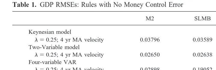
Counterfactual GDP simulations were conducted with three different economic models and three different policy instruments. In each simulation, the root mean square error of simulated nominal GDP from the targeted time path was computed. These RMSEs, along with RMSEs computed using historical data during the sample, appear in Table 1.
During the sample, the St. Louis monetary base and M2 always delivered greater levels of long-run price stability than actual discretionary monetary policy. Arguably, a com-parison of RMSEs simulated by rules to the RMSE of actual monetary policy from the 3%
target path biases the analysis in favor of the monetary rules. This occurs because historical monetary policy doesn’t target a stable price level. An alternative is to compare the relative ability of rules and discretionary monetary policy to reduce the variability of nominal GDP around a constant trend.17For rules, the constant trend is the targeted 3% GDP growth path. For discretionary policy, the constant trend utilized is the historical, 7.6% average rate of nominal GDP growth over the sample period.
Based on this comparison, the M2 rule still substantially reduced the variability of GDP about a fixed trend. The performance of the monetary base rules relative to historical monetary policy was model dependent. Historical policy outperformed both monetary base rules in the four-variable VAR, but not in the Keynesian and two-variable VAR models.
The St. Louis monetary base rule always outperformed the Federal Reserve Board monetary base rule. The source of this differential performance is probably due to (unreported) model estimation results which illustrate a stronger relationship between the St. Louis base and GDP than between the Board base and GDP.
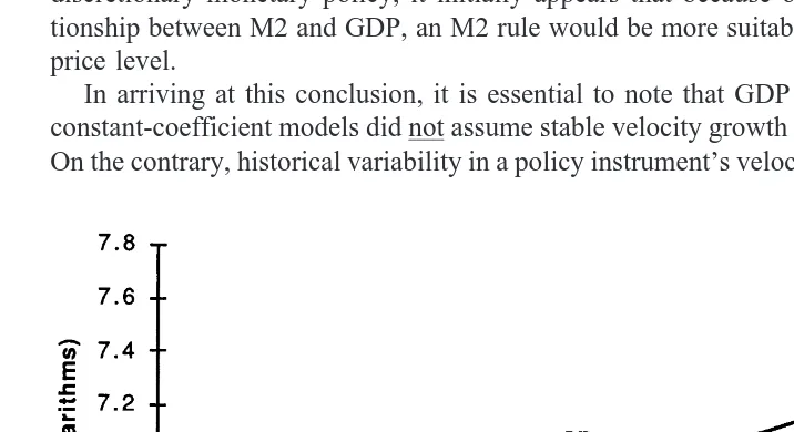
However, the performance of both monetary base rules deteriorated substantially in an economic model which also incorporated an interest rate. The relatively inferior perfor-mance of the monetary base and superior perforperfor-mance of M2 in the four-variable VAR model is not surprising. Dotsey and Otrok (1994) and Feldstein and Stock (1993) found that M2 is a significant predictor of nominal GDP— even when interest rates are included in the model. But Feldstein and Stock (1993) found that the predictive content of the St. Louis monetary base is eliminated, when interest rates are included in the model of nominal GDP determination. Although the base may have some predictive content for nominal GDP, this relationship is unstable. Consequently, Feldstein and Stock concluded that when interest rates are included in a model of GDP determination, the more stable interest rate relationship overwhelms the weaker relationship between the monetary base and GDP, causing the base to appear insignificant in models which include interest rates. The M2 rule performed well in all three economic models. The more stable relationship between M2 and GDP was not overwhelmed by the inclusion of interest rates in the model. Figures 1 and 2 illustrate the contrast between M2 and monetary base rules. In the
17It would be inappropriate to make a comparison of rules and discretionary policy based on simulations
using rules which target a nominal GDP growth path consistent with historical levels of inflation. Recall, one purpose of this study is to analyze the performance of rules which target a stable price level—not rules which target a stable inflation rate.
Table 1. GDP RMSEs: Rules with No Money Control Error
M2 SLMB FRBMB
Keynesian model
l50.25; 4 yr MA velocity 0.03796 0.03589 0.05375 Two-Variable model
l50.25; 4 yr MA velocity 0.02650 0.02638 0.04025 Four-variable VAR
l50.25; 4 yr MA velocity 0.02898 0.19052 explosive Historial GDP RMSE:
From a 3% growth path: 0.99288
From a 7.6%agrowth path: 0.15072
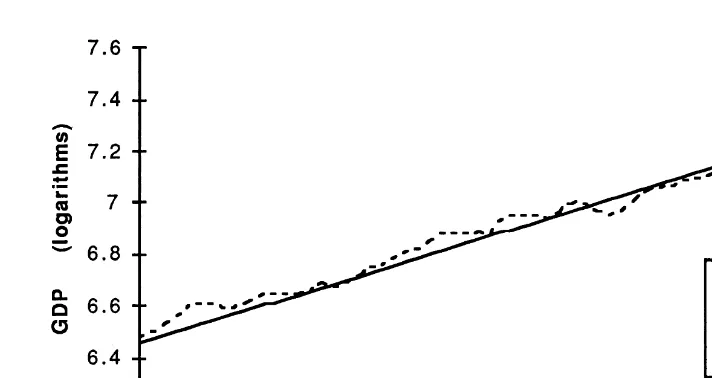
former case, simulated GDP closely tracks the target path. M2 appears to be a more robust policy instrument—in the case of no money control error. If the Fed were to adopt an adaptive rule or just utilize a rule to provide added information in the formulation of discretionary monetary policy, it initially appears that because of the more stable rela-tionship between M2 and GDP, an M2 rule would be more suitable for targeting a stable price level.
In arriving at this conclusion, it is essential to note that GDP simulations with these constant-coefficient models did not assume stable velocity growth over the sample period. On the contrary, historical variability in a policy instrument’s velocity growth rate affected
Figure 1. GDP growth path: M2 rule with no money control error in a four-variable VAR.
Figure 2. GDP growth path: St. Louis monetary base rule with no money control error in a
the GDP simulations through the size of the observations in the residual vectors (i.e., the GDP shocks). This point is particularly important given the recent debate about the reliability of M2 as a monetary policy indicator.18
During the 1980s, the Fed increasingly utilized M2 as a policy indicator because of its historically stable, long-run relationship with nominal income. Although the long-run average of M2 velocity had been trendless for decades, between 1990 and 1994, M2 velocity exhibited a seemingly transient change in its growth rate.19 The instability in velocity apparently was related to an expansion of financial assets which serve as substitutes for M2. In 1993, because of the instability in M2 velocity, Alan Greenspan announced the Fed was de-emphasizing M2 as a policy indicator. Yet, in McCallum’s Rule, M2 performed well between 1990 and 1995, keeping nominal GDP close to the target.20 Why?
As M2 velocity trended upwards, the GDP shocks in the macro models increased in size which tended to push simulated GDP away from the GDP target. But, in response, the four-year moving average velocity growth rate in McCallum’s rule gradually rose. This reduced the growth rate of M2 which then reduced deviations of nominal GDP from the target path. The feedback term in equation (1) provides an even more immediate monetary policy response to the changing velocity growth rate.
Greenspan’s 1993 announcement highlights a contrast between discretionary monetary policy, as recently implemented by the Fed, and McCallum’s Rule. The responses of the second and third terms on the right side of equation (1) make it unnecessary for M2 velocity to exhibit a pre-1990s level of stability, for the rule to successfully keep GDP close to the target. Although there presumably is a degree of velocity instability which would eradicate the success of the M2 rule, the most recent period of instability in M2 velocity did not exceed this critical threshold. As Section III demonstrates for M2, design features added purposefully by McCallum to make the rule fully operational adjust the growth rate of the policy instrument automatically to accommodate changes in velocity resulting from financial innovations, changes in the business cycle, or other sources.
In assessing the M2 rule, it is important to ask whether or not the favorable perfor-mance of M2, relative to the monetary base rule and discretionary monetary policy, persists in the face of money control errors. The performance of the M2 rule was reassessed assuming that money control error causes the actual growth rate of M2 to deviate from that specified by the rule. A likely explanation of money control error is that
18Carlson and Keen (1996) suggested utilizing MZM as an intermediate, target or indicator variable in the
formulation of monetary policy because MZM exhibited a stable demand function during the 1970s, 1980s and 1990s. (MZM is Money with Zero Maturity and equals M2 minus small time deposits plus institution-only money market mutual funds.) Unreported simulation results with an MZM version of McCallum’s rule indicate that MZM outperformed both measures of the monetary base only in the four-variable VAR model. But, MZM was outperformed by M2 in all three models and in the presence of money control error. Although MZM appears to be a stable function of its opportunity cost and real income, MZM demand is highly interest elastic and consequently, over time, MZM velocity varies over a much wider range than M2 velocity. Thus, the moving average term in McCallum’s rule more accurately forecasts current quarter values of the growth rate in M2 velocity—relative to its forecasts of MZM velocity growth. Therefore, the M2 rule delivers greater levels of price stability than the MZM rule. McCallum wanted his rule to be publicly observable. So, he specified velocity growth as a function of past changes in velocity, rather than movements in interest rates and real income. This design feature makes M2 preferable to MZM as a policy instrument.
19See Carlson and Keen (1995), Petersen (1995), and Mehra (1997).
20Figure 1 is a better guide to the performance of the M2 rule between 1990 and 1995 than the RMSEs in
the Fed generally prefers to attain the rule-specified, quarterly M2 target, but due to factors outside its control, this is sometimes impossible. When money control error is present, the value ofDMtthat enters into equations of GDP determination is defined as:
DMt5DRMt1MCEt (7)
where MCE is the money control error.21
To understand the operation of equation (7), for simplicity, assume that in time period (t21) nominal GDP does not deviate from the target. Thus, in equation (1), M5M2 and X*t215Xt21. Also assume that in time period (t), the four-year moving average growth rate of M2 velocity is 0. Then, in time period (t), the rule-determined, target growth rate of M2 is 0.00739 — or 3% in quarterly logarithmic units. Suppose in time (t), factors outside Fed control cause M2 growth to be below target. If M2 growth, measured in logarithms, is below target by 0.00249, MCEt5 20.00249. Using equation (7), we add 0.00739 to20.00249. So, in time (t), the growth rate in M2 which enters into the models of GDP determination is 0.00490 —about 2% in quarterly logarithmic units.
In order to realistically simulate GDP time paths, it is necessary to incorporate a likely measure of the money control error over the sample period. This requires specifying a process of monetary control for M2. Imprecise control over M2 forces the Fed to forecast how its policy actions (e.g., changes in the Federal Funds rate) will affect M2. Deucker’s (1995) model of monetary control is utilized to generate money control errors—assuming the Fed adjusts the federal funds rate to control M2.
Dln@Mt/~11FFRt!#5a01a1DTB3t211a2DTB10t211a3Dln Mt21
1a4D ln yt211 «8t. (8)
The change in the log of the money supply (i.e., M2), given the federal funds rate (FFR), is specified as a function of: a constant; the lagged change in the three-month Treasury bill rate (TB3); the lagged change in the ten-year Treasury bond rate (TB10); the lagged change in the log of M2 (M), and the lagged change in the log of real GDP ( y).
The initial vector of money control errors is generated by estimating equation (8) over the time period 1959:Q4 –1963:Q4 and then forecasting the subsequent quarter value of the dependent variable. The forecast is subtracted from the actual value of the dependent variable to generate the forecast error. The model is re-estimated, forecasts are generated, and forecast errors are computed using a rolling horizon approach until a vector of money control errors is generated for M2 over the sample period 1964:Q1–1995:Q4.
The rolling horizon approach was used to produce a time-varying coefficient model, which is desirable because the relationship between money growth and the federal funds rate varies in response to changes in the level of inflation, the economy’s position in the business cycle, etc. The M2, money control error vector derived this way had a mean of
20.00121 in quarterly logarithmic units (i.e.,20.5%) and a standard deviation of 0.0134 (i.e., 5.4%).22A random number generator was used to create a new money control error
21Although the specification of equation (7) indicates that the money control errors are added to the
rule-determined money growth rate, when the mean money control error is,0.0, the actual change in money growth tends to be below that specified by the rule.
22If one takes the midpoint of the M2 targets set since the mid-1970s, and compares actual growth to targeted
vector with the same statistical distribution as the forecast errors. This simulated error vector was recycled as the money control error vector in equation (7).23
Because the Fed can make changes in reserve requirements (e.g., place a uniform reserve requirement on all depository components of M2) and financial market regulations that would enhance its monetary control, this study doesn’t take the size of the money control error or its correlations with GDP shocks as given. More precisely, the question posed here is: given GDP shocks of historical magnitudes, how is the performance of an M2 rule affected by varying degrees of money control error? The goal of the analysis which follows is to determine if the realm of realistically-sized money control errors includes a threshold of controllability above which an M2 rule consistently produces more variation in nominal GDP (around a constant trend) than monetary base rules or historical discretionary monetary policy. This tests the operational capabilities of the M2 rule. To conduct this analysis, GDP simulations were conducted with different-sized money control error vectors.
The simulated M2 error vector was transformed to generate a grid of twenty-five different vectors of money control errors. The mean errors in the grid are22,21, 0, 1, or 2%. The standard deviations in the grid are 1, 2, 3, 4, or 5%. The grid encompasses the statistical distribution of money control errors generated by equation (8), but in response to arguments that the Fed can more precisely control M2, smaller standard deviations were also included in the grid of potential money control errors. In response to arguments that the Fed might use the existence of money control error as an excuse to violate the rule and pursue stealth discretionary policy, the grid also includes mean errors that are both larger and smaller than the mean money control error generated by equation (8). As the Fed has generally announced annual M2 targets within a band of 4%, the difference was split around the mid-point of the roughly 0% mean money control error generated by equation (8).
Correlation coefficients between the vectors of GDP shocks (generated by estimating each of the three economic models) and the initial M2 money control error vector (generated by equation 8) are roughly equal to zero. To generate error vectors which exhibited either a moderate positive or negative correlation with the GDP shocks of each economic model, the ordering of the values in the money control error vectors was altered.24For the three economic models, positive correlations between the money control error vector and the vector of GDP shocks ranged from 0.46 to 0.50. Negatively-correlated GDP shocks and money control errors were between20.50 and20.46, and uncorrelated errors ranged from20.003 to20.04.
GDP simulations were conducted with equations (1) and (7), in three different eco-nomic models, using the grid of twenty-five different money control error vectors outlined above. This yielded 75 simulations for money control errors which were: uncorrelated
23It is inappropriate to compute the money control error as the deviation of actual M2 from rule-specified
levels over the sample period. Errors computed this way would over-estimate the likely degree of money control error because at no time during this period was the Fed focusing explicitly on M2 as its single instrument of monetary policy. For similar reasons, it would also not make sense to compute the money control error based on deviations of historical M2 growth from the center of Fed specified targets.
24Rationality would dictate utilizing any information embedded in a systematic correlation between money
with GDP shocks, negatively correlated with GDP shocks, and positively correlated with GDP shocks.
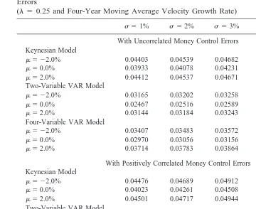
Results in Tables 2 and 3 report a subset of simulation results and indicate that the nature of the correlation between GDP shocks and money control errors affects rule Table 2. GDP RMSEs: M2 Rule with Uncorrelated and Positively-Correlated Money Control Errors
(l50.25 and Four-Year Moving Average Velocity Growth Rate)
s51% s52% s53% s54% s55% With Uncorrelated Money Control Errors
Keynesian Model
m5 22.0% 0.04403 0.04539 0.04682 0.04834 0.04986 m50.0% 0.03933 0.04078 0.04231 0.04394 0.04556 m52.0% 0.04412 0.04537 0.04671 0.04814 0.04958 Two-Variable VAR Model
m5 22.0% 0.03165 0.03202 0.03258 0.03333 0.03421 m50.0% 0.02467 0.02516 0.02589 0.02685 0.02795 m52.0% 0.03144 0.03184 0.03243 0.03322 0.03413 Four-Variable VAR Model
m5 22.0% 0.03407 0.03483 0.03572 0.03673 0.03780 m50.0% 0.02970 0.03056 0.03156 0.03270 0.03390 m52.0% 0.03714 0.03783 0.03864 0.03957 0.04056
With Positively Correlated Money Control Errors Keynesian Model
m5 22.0% 0.04476 0.04689 0.04912 0.05148 0.05382 m50.0% 0.04023 0.04261 0.04508 0.04766 0.05020 m52.0% 0.04501 0.04717 0.04944 0.05183 0.05420 Two-Variable VAR Model
m5 22.0% 0.03245 0.03381 0.03549 0.03747 0.03982 m50.0% 0.02572 0.02743 0.02951 0.03190 0.03440 m52.0% 0.03228 0.03370 0.03543 0.03750 0.03965 Four-Variable VAR Model
m5 22.0% 0.03364 0.03408 0.03473 0.03560 0.03661 m50.0% 0.02925 0.02978 0.03056 0.03158 0.03276 m52.0% 0.03682 0.03727 0.03793 0.03879 0.03978
Table 3. GDP RMSEs: M2 Rule with Negatively-Correlated Money Control Errors (l50.25 and Four-Year Moving Average Velocity Growth Rate)
s51% s52% s53% s54% s55% Keynesian Model
m5 22.0% 0.04259 0.04253 0.04258 0.04273 0.04297 m50.0% 0.03781 0.03779 0.03789 0.03810 0.03841 m52.0% 0.04287 0.04289 0.04301 0.04324 0.04354 Two-Variable VAR Model
m5 22.0% 0.03093 0.03074 0.03091 0.03144 0.03226 m50.0% 0.02384 0.02372 0.02406 0.02485 0.02598 m52.0% 0.03087 0.03088 0.03122 0.03193 0.03290 Four-Variable VAR Model
performance. In simulations where money control errors were either positively correlated or uncorrelated with GDP shocks, RMSEs increased as the mean and standard deviations of the money control error increased. Although the increase in the RMSEs across a given mean or standard deviation in the grid of money control errors was small, it was typically larger in the case of positive correlations. In these cases, there was only a very small increase in the variability of GDP and a very small reduction in the level of price stability attainable by the M2 rule. Even in the cases of the highest degree of money control error, during the sample period, the M2 rule still reduced the variability of nominal GDP by two-thirds, relative to historical monetary policy.
In the case of negatively-correlated money control errors and GDP shocks, in the Keynesian and two-variable VAR models, RMSEs increased slightly—suggesting that positive money control errors largely offset negative GDP shocks, and vice-versa. In the four variable VAR model, for any given mean error, the RMSE declined slightly as the standard deviation increased. Even when the money control error was largest, the M2 rule still reduced the variability of nominal GDP to about one-fourth of its historical value.
For all types of error correlations, the increases in RMSEs typically ranged from 0.5% to 2.0%, relative to the RMSE generated in the case of no M2, money control error. This is a very small increase in the RMSE, as is illustrated by Figure 3 which shows the GDP growth path generated by an M2 rule in the four-variable VAR model, in the case where money control errors are largest. In Figure 3, GDP exhibits only small and temporary deviations from the target path. Even during the period of velocity instability in the 1990s, simulated GDP deviates only slightly from target. The effects of a high degree of money control error, combined with positive correlations between the money-GDP shocks, was mostly mitigated by the feedback adjustment term, which produced subsequent quarter adjustments in M2 growth needed to keep GDP close to target.
Simulation results utilizing money control errors do not suggest the economy is insensitive to large changes in M2 growth. Rather, results indicate that the parameters in McCallum’s Rule are set at values which promote long-run price stability and signifi-cantly insulate the economy from undesired swings in money growth. Subject to some
Figure 3. GDP growth path: M2 rule with positively-correlated money control errors and GDP
caveats, addressed below, results suggest that, given GDP shocks of historical magnitudes (even those caused by the velocity shocks in the 1990s), the performance of an M2 rule is robust to varying degrees of money control error.
Findings regarding the likely success of an M2 rule are in contrast with those obtained by Dotsey and Otrok (1994)— even though both studies used money control errors of similar size. The most probable explanation is the use of different M2 rules. The adjustment parameters in McCallum’s rule appear to do a better job of mitigating the impacts of money control error on the GDP growth path.
To assess the relative performance of the policy instruments, it is useful to compare the RMSEs in Tables 2–3 with the RMSEs generated by corresponding economic models and monetary base rules. In the four-variable VAR, the M2 rule performed much better than either of the base rules.25When comparing monetary base and M2 rules it appears that even the addition of a plausible degree of money control error doesn’t much mitigate M2’s advantage of a relatively stronger and more stable relationship with nominal GDP (during this time period). The strength and stability of the relationship between the policy instrument and nominal GDP improves the ability of the feedback adjustment term to offset the undesirable impacts of money control errors. When comparing the performance of specific policy instruments, precise monetary control seems less advantageous than a stronger and more stable link to GDP.
In the Keynesian and two-variable VAR models, the St. Louis monetary base rule delivered slightly lower RMSEs than the M2 rule with money control error. But, this difference in performance is small and unlikely to be economically significant.
Results suggest that given current monetary control procedures, the Fed could suc-cessfully utilize an M2 rule to maintain much greater levels of price stability and much lower levels of GDP variability than we have achieved under discretionary monetary policy. The M2 rule is operationally sound and imposes the discipline necessary to achieve price stability. Findings also indicate that an M2 rule is likely to outperform a base rule.
IV. Caveats in the Analysis of an Adaptive M2 Rule
Conclusions regarding the likely ability of an M2 rule to increase price stability and lower the variability of nominal GDP around a constant trend are subject to many caveats.
All claims regarding the likely performance of any monetary policy rule are subject to the Lucas Critique. An elegant feature of McCallum’s Rule is that its ability to generate high levels of price stability and low levels of GDP variability is not contingent on the existence of unchanging coefficients linking the policy instrument to nominal GDP. To better understand this concept, suppose that implementation of an M2 rule by the Fed causes a one-time change in the historical relationship between M2 and nominal GDP. This would be reflected by changes in M2 velocity, which would be accommodated by the second and third terms in McCallum’s Rule. As long as the adoption of an M2 rule doesn’t
25The performance of a monetary base rule in VARs that incorporate an interest rate term seems to be
eliminate or excessively weaken the relationship between M2 and nominal income, the rule will automatically make the necessary adjustments.26
The apparent ability of the M2 rule to substantially increase price stability and reduce the variability of nominal GDP around a constant trend might be criticized on the grounds that the simple models used here overstate the strength of the relationship between M2 and nominal income. This criticism is contradicted by two arguments. First, recent studies (cited in Section II) on the relationship between M2 and nominal GDP have confirmed the existence of such a strong and stable relationship. Second, examinations of the empirical significance of the Lucas Critique show that some weakening of the strength of the relationship between M2 and nominal income doesn’t qualitatively change the result that the adaptive M2 rule could still produce sizable reductions in price instability and in the variability of nominal GDP.
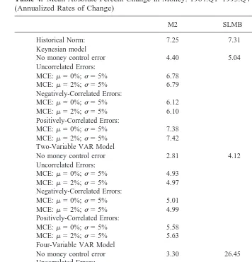
A third criticism is that the rules used here will produce greater variability in the policy instrument and, thus, real output than has been experienced historically. Using the mean absolute percent change (MAPC) in the policy instrument as a measure of variability, during the sample period the actual quarterly MAPC in M2 was 7.25% at an annualized rate. Table 4 illustrates that in the two- and four-variable VAR models, M2 would have been less variable under a rule. This result is robust for all sizes and types of money control error. In the Keynesian model, only in the case of positively-correlated GDP shocks and money control errors, was M2 slightly more variable then it has been historically. But, in the worst case, the MAPC rose to 7.42% at an annualized rate—a small increase. It appears that M2 is unlikely to vary more than it has historically.
By comparison, the historical MAPC of the St. Louis monetary base was 7.31% over the sample period. In the Keynesian model, the rule-determined MAPC was 5.04%; in the two-variable VAR model, it was 4.12%; but, in the four-variable VAR model it rose to 26.45%. The greater variability of the base in the latter model further illustrates that, unlike M2, the performance of the St. Louis base is not robust to the choice of economic model.
The likely variability of real GDP, resulting from the adoption of an M2 rule, can only be evaluated in the Keynesian and four-variable VAR. The historical MAPC of real GDP during 1964:Q1–1995:Q4 was 3.98%. The MAPC obtained with an M2 rule incorporating money control errors consistent with historical norms (i.e., with a mean of zero, a standard deviation of 5%, and uncorrelated with the GDP shocks) was 3.55%. Thus, in the four-variable VAR model, the variability of real GDP is slightly below the historical norm. The MAPC of real GDP obtained in the Keynesian model, with an M2 rule incorporating money control errors consistent with historical norms, was 4.76%. Although the MAPC increased in the Keynesian model, the increase was small. These results indicate that the benefits of price stability are not likely to be obtained at the costs of substantially increased instability in the policy instrument and/or in real output. This suggests that the costs of targeting a stable price level are likely to be small, further strengthening arguments for the adoption of an M2 rule.
26Examinations of the empirical significance of the Lucas Critique were conducted by McCallum (1988) and
V. Conclusion
The performance of different policy instruments (i.e., M2, the St. Louis, and Federal Reserve monetary base) has been examined using variations of McCallum’s adaptive rule for targeting levels of nominal GDP. Three economic models were used, respectively, to examine rule performance by simulating values of nominal GDP during 1964:Q1–1995: Q4. Rule performance was measured by the RMSE of simulated GDP from the non-inflationary target path.
Only the M2 rule appears to meet all four criteria for a successful policy rule. Unlike the monetary base rules, the M2 rule performed well (i.e., ensured long-run price stability) in a variety of plausible macroeconomic models—including one which incorporated an interest rate. The M2 rule performed well when financial innovations or other shocks altered the linkages between the policy instrument and the intermediate target. For example, even as M2 velocity growth changed in the early 1990s, causing an increase in Table 4. Mean Absolute Percent Change in Money: 1964:Q1–1995:Q4
(Annualized Rates of Change)
M2 SLMB FRBMB
Historical Norm: 7.25 7.31 7.36
Keynesian model
No money control error 4.40 5.04 5.78
Uncorrelated Errors:
No money control error 2.81 4.12 9.45
Uncorrelated Errors:
the size of the GDP shocks in the macro models, the M2 rule was able to adjust money growth and keep nominal GDP close to its target.
The M2 rule is also operational and compares favorably to historical discretionary policy in promoting long-run price stability. In comparison with historical, discretionary monetary policy, the M2 rule, with varying, likely degrees of money control error, substantially reduces the variability of GDP around a fixed trend—suggesting that the money control problem is mitigated by the strength and stability of the relationship between the policy instrument and GDP, and also by the feedback properties of the rule. These results strengthen the case for the adoption of an M2 rule to be used in the formulation of monetary policy— or at a minimum, to provide information useful in the formulation of discretionary monetary policy.
Helpful comments provided by Brian Madigan, Ray Fair, James Stock, Bennett McCallum, and two anonymous referees are gratefully acknowledged as is the research assistance of Adam Mueller and Sandy Hughes. Naturally, any errors are solely the responsibility of the author.
References
Aiyagari, S. R. Summer 1990. Deflating the case for zero inflation. Federal Reserve Bank of Minneapolis Quarterly Review 14:2–11.
Abate, J., and Boldin, M. 1993. The money-output link: Are F-tests reliable? Federal Reserve Bank
of New York Research Paper #9328.
Becketti, S., and Morris, C. Fourth Quarter 1992. Does money still forecast economic activity? Federal Reserve Bank of Kansas City Economic Review 77:65–77.
Carlson, J. B., and Keen, B. D. Dec. 1995. M2 growth in 1995: A return to normalcy? Federal Reserve Bank of Cleveland Economic Commentary
Carlson, J. B., and Keen, B. D. Second Quarter 1996. MZM: A monetary aggregate for the 1990s? Federal Reserve Bank of Cleveland Economic Review 32:15–23.
Clark, T. E. Third Quarter 1994. Nominal GDP targeting rules: Can they stabilize the economy? Federal Reserve Bank of Kansas City Economic Review 79:11–25.
Deucker, M. Jan./Feb. 1995. Narrow vs. broad measures of money as intermediate targets: Some forecast results. St. Louis Federal Reserve Bank Review 77:41–51.
Dickey, D., Jansen, D., and Thornton, D. 1994. A primer on co-integration with an application to money and income. In Co-integration for the Applied Economist (B. B. Rao, ed.). New York: St. Martin’s Press, 9–45.
Dotsey, M., and Otrok, C. Winter 1994. M2 and monetary policy: A critical review of the recent debate. Federal Reserve Bank of Richmond Economic Quarterly 80:41–59.
Engle, R., and Granger, C. W. March 1987. Co-integration and error correction: Representation, estimation, and testing. Econometrica 55:251–276.
Engle, R., and Yoo, B. 1987. Forecasting and testing in co-integrated systems. Journal of
Econo-metrics 35:143–159.
Fair, R. C., and Howrey, P. E. December 1994. Evaluating alternative monetary policy rules. Paper presented at 1995 AEA meetings.
Feldstein, M., and Stock, J. H. 1993. The use of a monetary aggregate to target nominal GDP. NBER
Working Paper #4304.
Friedman, B. 1988. Conducting monetary policy by controlling currency plus noise: A comment.
Friedman, B., and Kuttner, K. K. June 1992. Money, income, prices and interest rates. American
Economic Review 82:472–492.
Judd, J. P., and Motley, B. Summer 1991. Nominal feedback rules for monetary policy. Federal Reserve Bank of San Francisco Economic Review 2:3–17.
Judd, J. P., and Motley, B. Fall 1992. Controlling inflation with an interest rate instrument. Federal Reserve Bank of San Francisco Economic Review 3:3–22.
Judd, J. P., and Motley, B. 1993. Using a nominal GDP rule to guide discretionary monetary policy. Federal Reserve Bank of San Francisco Economic Review 3:3–11.
Marty, A., and Thornton, D. July/August 1995. Is there a case for ‘moderate’ inflation? Federal Reserve Bank of St. Louis Review 77:27–37.
McCallum, B. Sept./Oct. 1987. The case for rules in the conduct of monetary policy: A concrete example. Federal Reserve Bank of Richmond Economic Review 73:10–18.
McCallum, B. 1988. Robustness properties of a rule for monetary policy. Carnegie-Rochester
Conference Series on Public Policy 29:173–203.
McCallum, B. Aug. 1990. Could a monetary base rule have prevented the Great Depression?
Journal of Monetary Economics, 26:3–26.
McCallum, B. June 1993. Specification and analysis of a monetary policy rule for Japan. Unpub-lished manuscript. Carnegie-Mellon University, Pittsburgh, and NBER.
Mehra, Y. P. Summer 1997. A review of the recent behavior of M2 demand. Federal Reserve Bank of Richmond Economic Quarterly 83:27–43.
Petersen, D. J. Nov./Dec. 1995. FYI–Monetary aggregates, payments technology and institutional factors. Federal Reserve Bank of Atlanta Economic Review 80:30–37.
Rasche, R. 1995. Pitfalls in counterfactural analyses of policy rules. Open Economies Review, 6:199–202.
Thornton, D. March/April 1996. The costs and benefits of price stability: An assessment of Howitt’s rule. Federal Reserve Bank of St. Louis Review 78:23–38.
Thornton, S. Aug./Oct. 1993. Can forecast-based monetary policy be more successful than a rule?