Conditionally independent private information
in OCS wildcat auctions
Tong Li
!
, Isabelle Perrigne
",
*
, Quang Vuong
",#
!Indiana University, Los Angeles, USA"Department of Economics, University of Southern California, Los Angeles 90089-0253, USA #INRA, France
Received 1 May 1998; received in revised form 1 October 1999; accepted 1 October 1999
Abstract
In this paper, we consider the conditionally independent private information (CIPI) model which includes the conditionally independent private value (CIPV) model and the pure common value (CV) model as polar cases. Speci"cally, we model each bidder's private information as the product of two unobserved independent components, one speci"c to the auctioned object and common to all bidders, the other speci"c to each bidder. The structural elements of the model include the distributions of the common component and the idiosyncratic component. Noting that the above decomposition is related to a measurement error problem with multiple indicators, we show that both distributions are identi"ed from observed bids in the CIPV case. On the other hand, identi"cation of the pure CV model is achieved under additional restrictions. We then propose a computationally simple two-step nonparametric estimation procedure using kernel estimators in the"rst step and empirical characteristic functions in the second step. The consistency of the two density estimators is established. An application to the OCS wildcat auctions shows that the distribution of the common component is much more concentrated than the distribution of the idiosyncratic component. This suggests that idiosyncratic components are more likely to explain the variability of private
information and hence of bids than the common component. ( 2000 Elsevier Science
S.A. All rights reserved.
JEL classixcation: D44; C14; L70
*Corresponding author. Tel.: (213) 740 3528; fax: (213) 740 8543. E-mail address:[email protected] (I. Perrigne).
Keywords: Conditionally independent private information; Common value model; Non-parametric estimation; Measurement error model; OCS wildcat auctions
1. Introduction
Over the last ten years, the analysis of auction data has attracted much interest through the development of the structural approach. This approach relies on econometric models closely derived from game-theoretic auction models that emphasize strategic behavior and asymmetric information among participants. The structural econometrics of auction models then consists in the identi"cation and estimation of the structural elements of the theoretical model from available data. The structural elements usually include the latent distribu-tion of private informadistribu-tion while observadistribu-tions are usually bids. Previous studies have mainly adopted the independent private values (IPV) paradigm, where each bidder knows his own private value for the auctioned object but does not
know others'valuations which are independent from his.1An alternative
para-digm is the pure common value (CV) parapara-digm, where the value of the auctioned object is assumed to be common ex post but unknown ex ante to all bidders who have private signals about this value. It has been used in Paarsch (1992). More recently, Li et al. (1999) have extended the structural approach to the more
general a$liated private value (APV) model where bidders' private values are
a$liated in the sense of Milgrom and Weber (1982).
In this paper, we consider a model where a$liation among private informa-tion arises through an unknown common component. Speci"cally, we assume that each private information (either private values or signals) can be decom-posed as the product of two unknown independent random components, one common to all bidders and the other speci"c to each bidder. Because private information are independent conditionally upon the common component, the resulting model is called the conditionally independent private information (CIPI) model. As we shall see, the CIPI model is quite general and includes as special cases the conditionally independent private value (CIPV) model and the pure common value (CV) model.
The structural elements of the CIPI model include the distributions of the common and idiosyncratic components of private information. Considering a quite general model and decomposing private information render the identi-"cation and estimation of the structural elements from observed bids more
complicated than in previous studies such as Guerre et al. (2000) for the IPV model and Li et al. (1999) for the APV model. It turns out that identi"cation and estimation of the CIPI model is related to the measurement error model when many indicators are available as studied by Li and Vuong (1998). We show that the CIPV model is fully identi"ed nonparametrically. On the other hand, the identi"cation of the CV model requires some restrictions as the CV model is not identi"able in general from observed bids, see La!ont and Vuong (1996). In either case, combining Li et al. (1999) and Li and Vuong (1998) we propose a two-step nonparametric procedure for estimating the density of the idiosyn-cratic component and the density of the common component. In particular, our
procedure uses kernel estimators in the"rst step and empirical characteristic
functions in the second step. We then establish the consistency of our estimators. As an application, we study the Outer Continental Shelf (OCS) wildcat auctions. These auctions present some speci"c features which render the CIPI model relevant. On one hand, the common component can be viewed as the unknown expost value. On the other hand, the idiosyncratic component can be
considered as arising from a "rm's speci"c drilling, prospecting and
develop-ment strategies, capital and "nancial constraints, opportunity costs as well as
the precision of its own estimate of the value of the tract derived from geological surveys.
The structure of the CIPI model enables us to assess the roles played by both
the common and idiosyncratic components in"rms'bidding strategies.
Conse-quently, our approach complements previous studies done by Hendricks and Porter (see Porter, 1995 for a survey) who adopted the pure common value paradigm within a reduced form approach. In particular, comparisons of the distributions of the common and idiosyncratic components indicate that the idiosyncratic component explains a large part of the variability of bidders' signals, and hence of bids.
Our paper is original for several reasons. First, it contributes to the structural analysis of auction data as it shows that the structural approach can be extended to the CIPV and pure CV models. Second, from an econometric point of view, we propose an original method for estimating nonparametrically the latent distributions of each model that combines kernel methods and empirical charac-teristic functions. To our knowledge, the latter have been seldom used in empirical work. Third, we provide a new analysis of OCS wildcat auctions through a speci"ed structure of a$liation among valuations.
auctions with two bidders and present our empirical"ndings. Section 4 con-cludes the paper. Proofs are contained in an appendix.
2. The CIPI model and the structural approach
In this section, we"rst present the CIPI model as well as the related CIPV
and pure CV models. We then address their identi"cation from observed bids. Finally, we propose a two-step nonparametric procedure for estimating the underlying structural elements.
2.1. The CIPI,CIPV and CV models
We begin with the general a$liated value (AV) model introduced by Wilson (1977) and Milgrom and Weber (1982).
A single and indivisible object is auctioned to n*2 bidders. The utility of
each potential bidderi,i"1,2,n, for the object is;i";(pi,v) where;()) is
a nonnegative function strictly increasing in both arguments,p
i denotes theith
player's private signal or information andvrepresents a common component or
value a!ecting all utilities. The vector (p1,2,p
n,v) is viewed as a realization of
a random vector whose (n#1)-dimensional cumulative distribution function
F()) is a$liated and exchangeable in its"rstnarguments.2The distributionF())
is assumed to have a support [p
6, p6]n][v6,v6] withp6*0 andv6*0 and a density
f()) with respect to Lebesgue measure. Each playeri knows the value of his
signalpi as well asF()). However, he does not know the other bidders'private
signals and the common componentv.
In the CIPI model, it is assumed that bidders' private signalspi are
condi-tionally independent given the common componentv. Let F
v()) and Fp@v()D))
denote the cumulative distribution functions of v andp given v, respectively,
with corresponding densitiesf
v()) andfp@v()D)) and nonnegative supports [v
6, v6]
and [p
6,p6]. Hence in the CIPI model, the joint distributionF()) of (p1,2,pn,v)
is entirely determined by the pair [F
v()),Fp@v()D))] as
f(p1,2,p
n,v)"fv(v)Pni/1fp@v(piDv). (1)
It can be easily shown from (1) thatF()) is symmetric or exchangeable in its"rst
narguments and a$liated. Consequently, the CIPI model is a special case of the
general a$liated value model introduced by Wilson (1977) and Milgrom and Weber (1982).
We focus on the"rst-price sealed-bid auction, which is the mechanism used in the OCS wildcat auctions analyzed in this paper. As usual, we restrict our attention to strictly increasing di!erentiable symmetric Bayesian Nash
equilib-rium strategies. At such an equilibequilib-rium, playerichooses his bidb
i by
maximiz-ing E[(;
i!bi)1(Bi)bi)Dpi] where Bi"s(yi), yi"maxjEipj, s()) is the
equilibrium strategy, and E[)Dpi] denotes the expectation with respect to all
random elements conditional onp
i. As is well-known, the equilibrium strategy
satis"es the"rst-order di!erential equation
s@(p
i)"[<(pi, pi)!s(pi)]fy1@p1(piDpi)/Fy1@v1(piDpi), (2)
for all pi3[p
6,p6] subject to the boundary condition s(p6)"<(p6, p6), where
<(p
i,yi)"E[;(pi,v)Dpi,yi], Fy1@p1()D)) denotes the conditional distribution of y
1givenp1, andfy1@p1()D)) is its density. The index&1'refers to any bidder among
thenbidders because the game is symmetric. The distributionF
y1@p1()D)) is the
one corresponding to the probability structure de"ned in (1). As shown by Milgrom and Weber (1982), when the reservation price is nonbinding, the solution is
b
i"s(pi)"<(pi,pi)!
P
pip6
¸(aDpi) d<(a, a), (3)
where ¸(aDp
i)"exp[!:paify1@p1(uDu)/Fy1@p1(uDu) du]. It is easy to verify that b
i"Two important models are derived from the CIPI model. These are the CIPVs(pi) is strictly increasing inpi on [p6, p6]. model and the pure CV model.
2.1.1. The CIPV model
In this model, it is assumed that;(p
i, v)"pi so that each bidder's private information is his own utility, which he knows fully at the time of the auction.
We are thus in the private value paradigm and<(p
i, yi)"pi.
An economic interpretation of the CIPV model is as follows. Bidders'
valu-ations are independently drawn from a common distribution F
p@v()Dv) that
depends on an unknown parameterv. ThusF
v()) can be interpreted as bidders'
common prior distribution onv. In particular,vcan be interpreted as the ex post
value of the auctioned object for the average bidder while the discrepancy
between p
i and v results from bidder's speci"c characteristics such as his
productive e$ciency, opportunity costs, idiosyncratic preferences, etc. The CIPV model extends the IPV model by allowing for a$liation among bidders'
private values through the unknown common componentv. Because it speci"es
a special structure on a$liation, it is a special case of the APV model.3
3In fact, if one assumes that (p1,2,pn) are exchangeable for every n, then (p1,2,pn) are
The CIPV model formalizes the idea that a bidder who evaluates the object highly will expect others to evaluate it highly too. It is well suited to auction
situations, where there is some&prestige'value in owning the auctioned object
which is admired by other bidders and there is a possibility of resale at some currently undetermined price. These include auction of works of art, memor-abilia, collectibles, etc. In the case of OCS auctions, the auctioned tract adds to the capital of the winning oil company while the mineral content of the tract is
uncertain to the"rm.
2.1.2. The pure CV model
In this model, it is assumed that;(p
i, v)"vso that each bidder derives the
same but unknown utility from the auctioned object whilepiis bidderi's private
estimate of the common value. In this case,<(p
i,yi)"E[vDpi,yi"pi]. The economic interpretation of the pure CV model is well known. Di!erences
in bidders'preferences are neglected. On the other hand, bidders di!er through
their private information about the value of the auctioned object. This model has been frequently used to analyze auctions of drilling rights as the mineral content of the tract is subject to important uncertainty (see, e.g. Rothkopf, 1969, Wilson, 1977). As a result the model is sometimes called the mineral rights model (see Milgrom and Weber, 1982). In particular, oil companies are assumed to have di!erent estimates of the value of the tract, which are derived from geological surveys, but are assumed to have identical productive e$ciency, opportunity costs, etc.
2.2. Nonparametric identixcation
The structural approach relies on the hypothesis that the observed bids are the equilibrium bids of the auction model under consideration. Hence, the structural econometric model associated with the CIPI model is de"ned as
b
i"s(pi,;,Fv, Fp@v) for i"1,2,n, n*2, (4)
wheres()) is the equilibrium strategy (3). In particular, because private signals
are random and unobserved, bids are naturally random with ann-dimensional
joint distribution G()) determined by the structural elements of the model
[;()),F
v()),Fp@v()D))].
To implement the structural approach, a fundamental issue is whether the structural elements of the economic model are identi"ed from available
observa-tions. In general, all"rms'private information as well as the common
compon-ent are unknown to the econometrician, while only bids are observed. Therefore,
the identi"cation of the CIPI model reduces to whether the utility function;())
and the two underlying structural distributions F
v()) and Fp@v()D)) can be
determined uniquely from observed bids. An important feature of (4) is that the
F
v()) andFp@v()D)) in two ways: (i) through the unobservedpi, which is drawn
from F
p@v()Dv) while v is drawn from Fv()), and (ii) through the equilibrium
strategy, which is a complex function ofF()) and therefore ofFv()) andFp@v()D))
through (1) (see(3)). This feature complicates the analysis of identi"cation. Following a similar argument as in Li et al. (1999), denote the conditional
distribution ofB
1 givenb1 byGB1@b1()D)) and its density bygB1@b1()D)). Then
G
B1@b1(X1Dx1)"Pr(B1)X1Db1"x1)
"Pr(y
1)s~1(X1)Dp1"s~1(x1))
"F
y1@p1(s~1(X1)Ds~1(x1)).
It follows that
g
B1@b1(X1Dx1)" f
y1@p1(s~1(X1)Ds~1(x1)) s@(s~1(X
1))
.
Using the last two equations andp"s~1(b), the"rst-order di!erential equation
(2) can be written as
<(p, p)"b#GB1@b1(bDb) g
B1@b1(bDb)
,m(b,G). (5)
Recall that<(p,p)"E[;(p
1, v)Dp1"p,y1"p]. Thus a distinguishing feature
of (5) is that it expresses such an expected value as an explicit function of the
corresponding observed bid, the distributionG
B1@b1()D)) and densitygB1@b1()D))
of bids without solving the di!erential equation (2). The above equation forms the basis upon which the identi"ability of the CIPI, CIPV and CV models can
be studied.4
The next proposition relates the identi"ability of these three models. Here-after, we use the standard notion of observational equivalence of competing models from observables, which are here the observed bids. See La!ont and Vuong (1996) for a formal de"nition.
Proposition 1. Any CIPI model is observationally equivalent to a CIPV model. Hence, any pure CV model is observationally equivalent to a CIPV model.
The"rst part of Proposition 1 says that when explaining bids with condi-tionally independent signals, one can restrict oneself to a CIPV model without loss of explanatory power. The second part says that any interpretation in terms of the pure CV model can be equally given in terms of a CIPV model. This
proposition parallels Proposition 1 in La!ont and Vuong (1996), which relates AV to APV models. The di!erence here is that private signals are now assumed to be conditionally independent, which leads naturally to the CIPI and CIPV models. Intuitively, to establish that any CIPI model is observationally
equiva-lent to a CIPV model, the argument is that;(p
i, v) can be replaced by;I i"p8i,
wherep8
i"<(pi, pi) are conditionally independent givenv. In other words,;())
is not identi"ed. Thus, we focus below on the CIPV and pure CV models where
;(p,v)"pand;(p,v)"v, respectively.5
As noted by La!ont and Vuong (1996, Proposition 4), however, the pure CV model is not identi"ed. Similarly, it can be shown that the CIPV model is not
identi"ed either. Intuitively, the conditioning variablevin a CIPV model can be
replaced by any strictly increasing transformation ofvwhile retaining the same
probabilistic structure on the utilities (p1,2,pn). This implies that additional
restrictions are needed for identi"cation. Assuming that signals are unbiased is not su$cient by itself. In this paper, we assume the multiplicative decomposition
pi"vgi, wherevis the common component andgi is speci"c to theith bidder. Moreover, the following assumptions are made.
A1: Theg
i's are identically distributed with a mean equal to one.
A2: vand thegi's are mutually independent.
The mean requirement in Assumption A1 is a natural normalization and ensures that the signals are unbiased estimates of the common component as in
Wilson (1977). Together Assumptions A1 and A2 imply that private signalsp
i's
are independent and identically distributed conditionally uponv. The structural
elements of either model are now the pair [F
v()),Fg())], where Fg()) is the
cumulative distribution ofgwith support [g
6, g6] so that [p6, p6]"[vg,v6 g6].6
2.2.1. Identixcation of the CIPV model
As noted earlier, the CIPV model is a special case of the APV model. From the nonparametric identi"cation of the APV model (see Li et al., 1999, Proposi-tion 2.1), it follows that the joint distribuProposi-tion of private values in the CIPV model is identi"ed from observed bids. The remaining question is whether the
structural elements [F
v()),Fg())] of the CIPV model are uniquely determined
5Given the similar probabilistic structure of the CIPV and pure CV models, an interesting question is whether any CIPI model is observationally equivalent to a pure CV model. A positive answer would imply the converse of the second part of Proposition 1. At this stage, however, it is not known whether such a conjecture is true.
6See also Wilson (1998). An alternative decomposition for private signals ispi"v#g
iwith the
by such a joint distribution. To address this question, we note that the
multipli-cative decomposition leads to logpi"logc#logei, where
logc,[logv#E(logg)], loge
i,[loggi!E(logg)], (6)
i"1,2,n*2, and logei has zero mean. Hence, under Assumptions A1}A2,
this problem is related to an error-in-variable model with multiple indicators.
Indeed, loge
i can be considered as the error term in the classical measurement
error model where logcis unobserved. Because thep
is can be recovered from
observed bids through (5) where <(p, p)"p, their logs can be viewed as
indicators for logc.
When the densities for logcand logeare both unknown, the error-in-variable
model with multiple indicators is nonparametrically identi"ed under a mild additional condition (see Li and Vuong, 1998, Lemma 2.1). In our context, such a condition is satis"ed under the following assumption.
A3: The characteristic functions/
v()) and/g()) of logvand loggare
nonvan-ishing everywhere.
Such an assumption is standard in the related deconvolution problem with
/
g()) known and only one indicator (see, e.g. Fan, 1991; Diggle and Hall, 1993
for recent contributions).7 From Li and Vuong's (1998) identi"cation result,
which relies upon Kotlarski's result (see Rao, 1992, p. 21), we have immediately the following lemma, which will be also useful in the estimation part.
Through-out, we useh
x()) to denote the density of logx, keepingfx()) for the density ofx.
Lemma 1. Given A1}A3, the densitiesh
c())andhe())are uniquely determined by
the joint distribution of an arbitrary pair (logp1, logp2). Their characteristic functions are
/
c(t)"exp
P
t0
Lt(0,u
2)/Lu1
t(0,u
2)
du
2, (7)
/
e(t)"
t(0, t)
/
c(t)
"t(t, 0)
/
c(t)
, (8)
wheret(t
1,t2)is the characteristic function of(logp1, logp2).
The identi"cation result in Lemma 1 is useful because not only are the
densitiesh
c()) andhe()) of logcand logeidenti"ed by the joint distribution of
(logp1, logp2), but explicit formulae for the characteristic functions of these
densities are also available.8
The next proposition establishes the identi"cation of the CIPV model and characterizes the restrictions on the distribution of observed bids that are imposed by the CIPV model. In particular, it uses Lemma 1 and the equality
E(logg)"!log E(e), which results from the normalization condition E(g)"1.
Proposition 2. Given A1}A3, the CIPV model is identixed. Moreover,a distribution of observed bids can be rationalized by a CIPV model if and only if (i)bids are symmetric and conditionally independent, and (ii) the function m(),G) is strictly
increasing on[b
M, bM].
2.2.2. Identixcation of the pure CV model
The next proposition establishes the partial identi"cation of the pure CV model under the following assumption.
A4. <(p,p) is loglinear in logp, i.e. log E[vDp
1"p, y1"p]"C#Dlogp,
where (C, D)3R]RH
`.9
The usefulness of A4 under the multiplicative decomposition can be seen by
noting that log E[vDp
i, yi"pi]"logc#logei, where logcand logei are now de"ned as
logc"C#DE(logg)#Dlogv, loge
i"D[loggi!E(logg)], (9)
where E(logg)"!log E(e1@D) using the normalization E(g)"1.
Proposition 3. Given A1}A4, the distributions ofvandgare given by
logv"log E[e1@D]!C
D#
1
Dlogc, logg"!log E[e1@D]#
1
Dloge,
where the distributions of c and e are identixed from observed bids through Lemma 1 with t(t
1, t2) being now the characteristic function of
(log<(p
1, p1), log<(p2, p2)) (say).
Proposition 3 says that, up to (C, D) which determine the location and scale,
the distributions of logvand loggare uniquely determined from observed bids.
Moreover, because the scale is common, the ratio Var(logg)/Var(logv) is
inde-pendent of (C,D) and equal to the ratio Var(loge)/Var(logc). Since the latter is
8As indicated in Li and Vuong (1998), an alternative way to establish the identi"ability of (h
c()),he())) consists in showing that all moments of logcand logeare identi"ed from the moments
of the joint density of logp1, logp2. For instance, E[logc]"E[logp1]"E[logp2], E[log2c]"E[logp1logp2], E[log2e]"E[log2p1]!E[logp1logp2], etc.
9Because of a$liation, E[vDp1"p,y
identi"ed, it can be used to assess the relative variability of bidders'idiosyncratic component and the common value.
It remains to discuss when A4 is satis"ed, which will provide additional
information on (C, D). A leading case when A4 holds is when the prior on the
common value is inversely proportional tovc, i.e.f
v(v)J1/vc,c3R. In this case,
it can be shown (see Appendix) that
log E[vDp1"p, y
so thatD"1. Whenc"2 and a homogeneity assumption on the distribution of
signals holds, which is satis"ed here by the multiplicative decomposition, Smiley (1979) has shown that the bidding strategy is proportional to the signal. Using Smiley's result, Paarsch (1992) proposes a parametric estimation of the pure CV model. Assumption A4 is much more general and allows for nonlinear bidding strategies.
Another case when A4 holds occurs with two bidders (n"2) when (v, g1, g2)
is jointly log-normally distributed with parameters (kv,p2
v, kg, p2g) and
Moreover, from (9) the distributions ofcandeare log-normal with parameters
(k
The preceding results are important for several reasons. First, for the CIPV model, we have achieved full nonparametric identi"cation result of the underly-ing structural distributions. Second, for the pure CV model, we have proposed partial nonparametric identi"cation results, which are the most general to date. Third, in both cases, we can assess the relative variability of the common
10Under the additive decomposition pi"v#g
i, A4 is replaced by the linearity in p of
E[vDp1"p,y
1"p]. By a similar argument used for establishing (10), it can be easily shown
that such an assumption A4@ is satis"ed with a #at prior on v in which case E[vDp1"p,y
1"p]"!E[g1Dg1"maxjE1gj]#p. Alternatively, whenn"2, A4@is satis"ed if
component and the idiosyncratic component in bidders' private information.
Fourth, it is interesting to note that provided one knowsG, one has neither to
solve the di!erential equation (2) nor to apply numerical integration in (3) so as
to determine<(p, p). For knowledge ofG()) and hence of m(), G) determines
either the private valuepin the CIPV model or E(vDp1"p, y
1"p) in the pure
CV model for any given bid through (5) and, hence the distributions of the common and private components, respectively. Eqs. (5), (7) and (8) form the basis upon which the nonparametric procedure proposed in the next sub-section rests.
2.3. Nonparametric structural estimation
We now propose a two-step nonparametric procedure for estimating the
densities h
c()) and he()). Note that these determine uniquely the structural
densities h
v()) and hg()) in the CIPV model through (6) since
E(logg)"!log E(e) from the normalization E(g)"1. On the other hand, up to
C and D which determine the location and common scale, the structural
densitiesh
v()) andhg()) in the pure CV model can be recovered from
Proposi-tion 3. Also, because we do not impose any parametric restricProposi-tion on the underlying densities, our nonparametric estimation procedure is equivalent to
estimating them separately for each number of bidders.11
The basic idea of our two-step estimation procedure is to use (5) followed by
Lemma 1. Speci"cally, if one knewG
B1@b1()D)) andgB1@b1()D)), then one could use
(5) to recover<
i,<(pi, pi) for bidderi, i"1,2,n, which is the private value
p
iin the CIPV model and the expectation E[vDpi,yi"pi] in the pure CV model.
These can be used to estimate the joint characteristic function of (log<
1, log<2)
(say). Hence nonparametric estimates of densities of interest can be obtained from Lemma 1 through (7)}(8). Hence, our estimation procedure is as follows:
Step1: Construct a sample based on (5) using nonparametric estimates of
G
B1@b1()D)) andgB1@b1()D)) from observed bids.
Step2: Use the pseudo sample in logarithm constructed in Step 1 to estimate
nonparametrically h
c()) and he()) via their estimated characteristic
functions. These are then used to estimateh
v()) andhg()) for either
model.
To be more speci"c, letnbe a given number of bidders. Let¸be the number of
auctions corresponding to the chosen n, and let l index the lth auction,
11That is, our procedure estimatesh
v@n()Dn) andhg@n()Dn) for each value ofn. In practice, auctioned
l"1,2,¸. In Step 1, using the observed bidsMbil;i"1,2,n; l"1,2,¸N,
we estimate nonparametrically the ratio G
B1@b1()D))/gB1@b1()D)) by
kernels. Using (5) we obtain estimates of the unobserved<
il as
Step 1 is similar to the "rst step in the two-step nonparametric estimation
procedure of the APV model proposed in Li et al. (1999). As mentioned by Guerre et al. (1999), some trimming is necessary in order to correct for the boundary e!ects caused by the density estimate in the denominator of (15). Such a trimming is presented in Section 3.2 A consequence of the trimming is that it reduces the number of estimates and hence the number of auctions that can be
used in Step 2. Let¸
T be the number of auctions after trimming.
We now turn to Step 2, which is composed of three substeps.
f Substep 1. Estimate the joint characteristic function of any two bidders'
log<
f Substep 2. Estimateh
c()) andhe()) by
f Substep 3. Estimates of the structural densities are obtained in the CIPV
model by
hK
v(x)"hKc[x#EK(logg)], hKg(y)"hKe[y!EK(logg)],
where EK(logg)"!log EK(e). In the pure CV model, they are obtained as
hK
v(x)"DhKc[D(x#(C/D)!log EK(e1@D))],
hKg(y)"DhKe[D(y#log EK(e1@D))],
given (C,D).
In Li and Vuong (1998), the uniform consistency of the nonparametric
estimators proposed in Step 2 is established when the &indicators' <
il are
observed. This is done by assuming that the densities of interest are either ordinary or super-smooth through the tail behavior of their characteristic functions. Following Fan (1991), we have
Dexnition 1. The distribution of a random variableZ is ordinary smooth of
orderb if its characteristic function/
Z(t) satis"es
d
0DtD~b)D/Z(t)D)d1DtD~b
astPRfor some positive constantsd
0, d1,b.
On the other hand, it is super-smooth of orderbif /
Z(t) satis"es
d
0DtDb0exp(!DtDb/c))D/Z(t)D)d1DtDb1exp(!DtDb/c)
astPRfor some positive constantsd
0, d1,b, cand constantsb0 andb1.
Speci"cally, we make the following assumption.
A5. The characteristic functions /
v()) and /g()) are ordinary smooth with
b'1 or super-smooth.
Note that the characteristic functions/
v()) and /g()) are necessarily both
integrable. In addition, Li and Vuong (1998) make the next assumption, which we maintain here.
A6. The supports ofh
v()) andhg()) are bounded intervals ofR.
Unlike in Li and Vuong (1998), the indicators<
ilare unobserved. Instead, we
use their estimates<K
ilobtained in Step 1. Moreover, the pseudo values used in
Step 2 are trimmed to correct for boundary e!ects. Nonetheless, we can still establish the following result.
Theorem 1. Under A1}A6,hKc())andhKe())are uniformly consistent estimators for
h
inxnity as ¸PR. Hence, if C and D are known, hKv()) andhKg())are uniformly
consistent estimators forh
v())andhg())in either the CIPV or pure CV model.13
The proof of Theorem 1 is given in Appendix. It relies on an important lemma,
which establishes the uniform convergence of the estimator (19) on [!¹,¹].
This is proved using the log-log law and von Mises di!erentials.
3. Application to the OCS wildcat auctions
In this section, we illustrate our estimation results on OCS wildcat auctions
with two bidders.14 A "rst subsection brie#y discusses the data. A second
subsection deals with some practical issues for implementing our structural
estimation procedure. Our empirical"ndings within either the CIPV or the pure
CV model are discussed in a third subsection.
3.1. Data
The U.S. federal government began auctioning its mineral rights on oil and
gas on o!shore lands o!the coasts of Texas and Lousiana in the gulf of Mexico
in 1954. In this application, we focus on wildcat tracts sold through sales held between 1954 and 1969. This gives us a total of 217 auctioned wildcat tracts with two bidders.
Before each sale, the government announces to oil companies that an area is available for exploration. This area is divided into a number of tracts, each of which is usually a block of 5000 or 5760 acres. Firms are allowed to get limited information about tracts using seismic surveys and o!-site drilling. However, no drilling is allowed on each tract before the auction. Because bidders have equal access to the same information about the tract, they can be considered as identical ex ante so the game is symmetric (see McAfee and Vincent, 1992 for more details).
13In the CIPV model, Assumption A4 is automatically satis"ed withCandDknown (and equal to zero and one, respectively) since log<(p,p)"logp. In the pure CV model, the assumption that CandDare known is restrictive. IfCandDare unknown, however,h
v()) andhg()) are estimated
consistently up to location and common scale by hKc()) and hKe()), as mentioned earlier. The
appropriate divergence rate of¹is given in the appendix, Lemma A.1.
14Recall that our procedure can provide estimates ofh
v@n()Dn) and hg@n()Dn) for each value of
n"2, 3,2. Thus, in this case we estimatehv@n()D2) andhg@n()D2) as auctions with two bidders provide
us with the largest number of bids. Because the"rst step involves estimating a bivariate density (see (14)), the curse of dimensionality and data availability prevent us to considern'3. If one is willing to accept the hypothesis thatnis exogenous so thath
v@n()Dn) andhg@n()Dn) are independent ofn, one
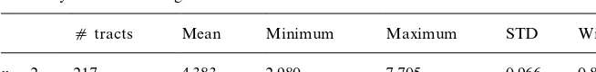
Table 1
Summary statistics for log bids
dtracts Mean Minimum Maximum STD Within STD
n"2 217 4.383 2.980 7.705 0.966 0.875
The U.S. federal government organizes a"rst-price sealed-bid auction for the
lease of drilling rights. Firms submit their bids, the highest bid wins the tract and the winner pays his bid provided his bid is higher than the reserve price announced prior to the auction. In principle, the presence of a reserve price induces a discrepancy between the number of actual bidders and the number
nof potential bidders considered in auction theory. However, in OCS auctions
the announced reserve price of$15 per acre has been acknowledged to be very
low by all researchers in the"eld (see, McAfee and Vincent, 1992 and the work
by Hendricks and Porter). Hence the reserve price does not act as an e!ective screening device for the participation of bidders. Likewise, the federal govern-ment has the right to reject the highest bid in any auction. Only 1.8% out of the 217 auctions were rejected, which indicates that this rejection rule does not have much e!ect on bidding strategies. Lastly, the federal government allows the practice of joint bidding, which could introduce some ex ante asymmetry among bidders. Only 23 tracts out of the 217 tracts received one joint bid and 9 of them were won by a joint bid. The ratio 9/23 is not statistically di!erent from 1/2. Hence joint bidding does not seem to have introduced asymmetries. Conse-quently, we can consider that the framework presented in Section 2.1 constitutes
a reasonable"rst approximation for our application.
We now turn to the data set used (see Hendricks et al., 1987 for a more detailed description of the complete data set). For each auctioned wildcat tract, we know in particular its acreage, the number of bidders, and their bids in constant 1972 dollars. As Li et al. (1999) have shown through a regression of the log of bids per acre on a complete vector of tract speci"c dummies, tract heterogeneity becomes insigni"cant conditionally on the number of bidders. That is, for auctions with a given number of bidders, one can consider that bids
variability is mainly due to di!erences among "rms and not to di!erences
among tracts. Table 1 provides some summary statistics on the log of bids analyzed hereafter.
Table 1 shows that the overall standard deviation (STD) is largely due to the
within standard deviation.15 This indicates a large variability of bids within
15The (average) within standard deviation (STD) for tracts withnbidders is computed as the square root of (1/(¸(n!1)))+Ll
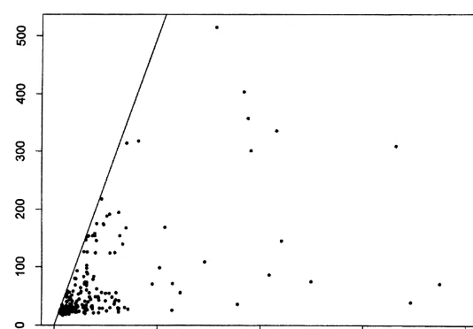
Fig. 1. Pairs (b
1,b2) withb1*b2.
tracts as can be seen from Fig. 1, which plots all the pairs (b
1,b2) withb1*b2.
A regression of the 434 log of bids on 217 tract dummies gives anF-test of the
equality of all tract dummies of 1.55 with (216, 217) degrees of freedom, which is
barely signi"cant at the 1% level.16
3.2. Some practical issues
To implement our estimation procedure, a number of practical issues have to be addressed. First, while the range of bids for tracts with two bidders is
[19.70, 2220.28] in$per acre, we observe a high concentration (about 70%) of
observations in the interval [20, 200], i.e. a highly skewed distribution of bids. To avoid trimming out many observations, we transform the data using the logarithmic function. With such a transformation, (5) becomes
<(p, p)"exp(a)
A
1#GA@a(aDa)g
A@a(aDa)
B
!1,q(a) (21)
where a,log (1#b), G
A@a()D)) is the conditional distribution of
max
i/2,2,nlog (1#bi) given log (1#b1), andgA@a()D)) is its density. Using the
trimming introduced in Guerre et al. (1999), the pseudo values<K
il. This trimming is necessary in view of boundary e!ects in
kernel estimation.17 As in Section 2.3, the nonparametric estimates GK
A,a(),))
andg(
A,a(),)) are obtained from (13) and (14), with the exception that all bids are
now in log (1#b). The second step of our estimation procedure only uses the
pseudo values that are"nite as de"ned in (22). We now discuss the pratical issues
speci"c to the"rst and second steps.
In the"rst step, we need to address the choice of the kernel functionsK
Gand
K
gand their corresponding bandwidthshGandhg. Though the choice of kernels
does not have much e!ect in practice, we choose a kernel with compact support that is continuously di!erentiable on its support including the boundaries so as to satisfy the assumptions in Guerre et al. (1999). Numerous kernel functions satisfy these properties (see Hardle, 1991). This is the case for the triweight kernel de"ned as
K(u)"35
32(1!u2)31(DuD)1). (23)
ThusK
g is de"ned as the product of two univariate triweight kernels.
In contrast, the choice of the bandwidths requires more attention. From the
rates given in Li et al. (1999), we use bandwidths of the formh
G"cG(n¸)~1@5
andh
g"cg(n¸)~1@6. Note that these rates correspond to the usual ones so that
c
Gandcg can be obtained by the so-called rule of thumb. Speci"cally, we use
h
G"2.978]1.06p(a(n¸)~1@5 and hg"2.978]1.06p(a(n¸)~1@6, where p(a is the
standard deviation of the logarithm of (1#bids), and the factor 2.978 follows
from the use of the triweight kernel instead of the Gaussian kernel (see Hardle,
1991). Thus h
G and hg are equal to 0.9049 and 1.1079, respectively. After
performing the"rst step estimation and the trimming on the pseudo values<K
il,
we"nd that the trimmed values have a mean equal to$253.41 per acre, while the
17We assume thatp
6"0. Hence,bM"0 in view of (3) and A4. The transformation log (1#)) then ensures thata
6"0 and that the support [a6,a6] is compact as soon asbM(R, i.e. as soon asp6(R becausebM"s(p6). Thus we do not need to estimate the lower bounda
minimum and maximum are 19.73 and 1181.38, respectively. After trimming, 174 auctioned tracts remain out of 217.
In the second step, some new practical problems are encountered. First, the use of empirical characteristic functions for estimating their corresponding densities typically produces many oscillations because of the large range of values estimated in Step 1. To mitigate this problem, we divide the logarithm of
all pseudo values<K
ilby 7 so as to get an interval close to [0, 1]. Second, as noted
by Diggle and Hall (1993), the estimators (17) and (18), which are obtained by
truncated inverse Fourier transformation, may have some sharp #uctuating
tails. Such an unattractive feature can be alleviated by adding a damping factor to the integrals in (17) and (18). Following Diggle and Hall (1993), we introduce a damping factor de"ned as
d(t)"
G
1!DtD/¹ if DtD)¹,0 otherwise. (24)
Thus, estimators (17)}(18) are generalized to
hKc(x)"1
2p
P
T
~T
d(t)e~*tx/Kc(t) dt, (25)
hKe(y)"1
2p
P
T
~T
d(t)e~*ty/Ke(t) dt. (26)
In practice, this damping factor will&smooth'the tails of our density estimators.
Third, though the smoothing parameter¹can be chosen to diverge slowly as
¸PR so as to ensure the uniform consistency of our estimators, the actual
choice of¹in"nite samples has not yet been addressed in the literature. Indeed,
¹plays here the role of a smoothing parameter, as large (small)¹will produce
undersmoothing (oversmoothing) of the density estimate. In our case, ¹ is
chosen through some empirical or data-driven criterion. As mentioned in
footnote 8, we can obtain estimates for all moments of logcand logefrom the
moments of (log<
1, log<2). Hence, using the trimmed pseudo sample of values
obtained in Step 1, we can obtain estimates of the means and variances of logc
and loge as k(
c"4.937,k(e,0,p(2c"0.00222 and p(2e"0.02195. These two
estimates can then be used to choose a value of¹. Speci"cally, we try di!erent
¹'s and obtain corresponding estimates of h
c()) and he()) through (25)}(26).
From each estimated density, we compute the corresponding means and
vari-ances k8c, k8e, p82c and p82e, respectively. This gives the goodness-of-"t criterion
Dp82c!p(2cD#(k8c!k(
c)2 for c, and similarly for e. The value of ¹ we choose
minimizes the sum of these errors in percentage ofp(2c andp(2e. This gives¹equal
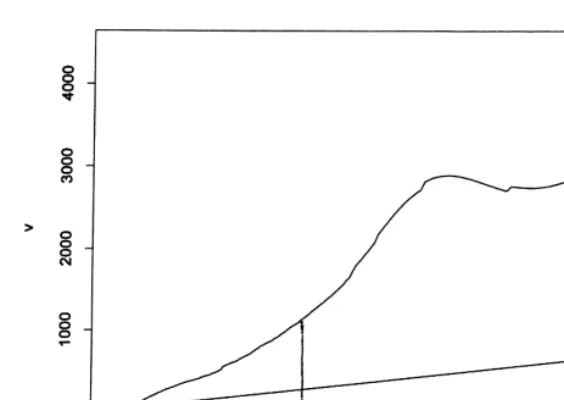
Fig. 2. EstimatedmK()) function.
3.3. Empiricalxndings
The structural approach adopted in this paper allows us to recover the two
crucial densities, namely,h
c()) andhe()). These in turn allow us to determine the
density of the common componentvand the density of the private component
giin both the CIPV and pure CV models, providedCandDare known in the
latter case. As noted earlier, ifCandDare unknown, the densities of logvand
loggare recovered up to location and common scale only. In the OCS case, the
economic interpretation is as follows. Whilevcan be viewed as the expost net
value of the tract for the average"rm, gi is due to"rm's private information
about the tract, which include"rm's productive e$ciency, opportunity costs in
the CIPV model, or"rm's idiosyncratic estimate in the pure CV model. Thus,
a positiveg
iindicates that"rmihas a higher (expected) value for the tract given
his private information due to either higher e$ciency and lower opportunity costs in the CIPV model, or higher estimate in the pure CV model.
Fig. 2 displays the estimated function mK()), which is the inverse of
the equilibrium strategy. The vertical line corresponds to the value
exp(d
.!9!2 maxMhG,hgN), which de"nes our upper trimming (see (22)). About
85% of the observed bids are below this upper trimming value. Though the
functionmK()) is not always increasing, a striking feature of Fig. 2 is that it is
strictly increasing on [0, exp(d
.!9!2 maxMhG,hgN)], which corresponds to the
region wherem()) is well estimated. In view of Proposition 2, it follows that the
Fig. 3. Estimated density of<
il.
agreement with the monotonicity of the bidding strategyb"s(p) in the pure CV
model.18
In continuous line, Fig. 3 displays the nonparametric estimate of the density
of the trimmed log<K
ils using the triweight kernel (23) with a bandwidth given by
h"2.978]1.06p(
V(n¸T)~1@6, wherep(V"1.088 is the standard deviation of the
trimmed log<K
il's.19For comparison, in dotted line we also display the normal
density with mean equal to 0.494 (the empirical mean of the trimmed log<K
il's)
and standard deviationp(
V"1.088. Fig. 3 indicates that the estimated density of
log<
ilis not normal with two modes. Since log<
i"logc#logei, it follows that
the distributions ofcande(and hence ofvandg) cannot be both log-normal. As
a matter of fact, from CrameHr (1936), none of these distributions can be
log-normal.
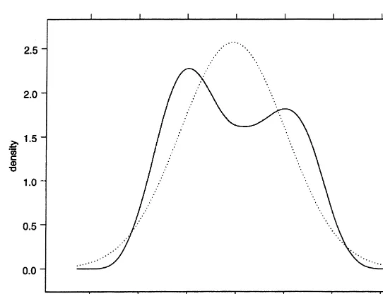
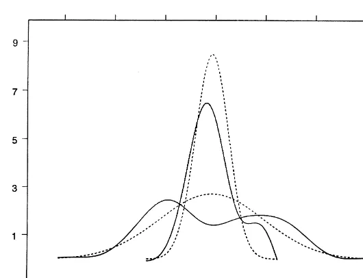
Fig. 4 displays the estimates ofh
c()) andhe()) in continuous lines. Though the
mean of logeis zero by de"nition, its estimated densityhK
e()) has been centered
around the estimated mean k(
c"4.937 of logc to facilitate comparison.
Sim-ilary, Fig. 4 displays the normal densities with common meank(
c"4.937 and
variancesp(2c"0.00222 and p(2e"0.02195. Fig. 4 con"rms our earlier"nding
that neither the density ofcnor the density ofeis log-normal. Indeed, the density
hKc()) displays a bump in its right tail, whilehKe()) has two modes. Moreover, the
18See Hendricks et al. (1999) for a recent contribution to testing the pure CV model.
Fig. 4. Estimated densitieshKc()) andhKe()).
former is much less spread out that the latter with a variance about ten times smaller.
As logvand loggare related to logcand logethrough linear transformations
with a common scale factor (see (6) and (9)), the preceding"ndings apply to the
structural densitieshK
v()) andhKg()) as well. In particular, whether the CIPV or
pure CV model is adopted, we "nd that the "rms' prior distribution of the
common componentvis ten times less spread out (as measured by the variance
of the density of the logarithm) than the distribution of "rms' idiosyncratic
componentg. Such a result agrees with previous empirical studies stressing the
variability of"rms'private information as the main source of bids'variability in
OCS auctions (see, e.g. Hendricks et al. (1987) in the pure CV model, and Li et al. (1999) in the APV model).
Fig. 4 also indicates that the estimated density of logvis essentially
single-peaked, while the estimated density of logghas two modes. This suggests that,
whatever the paradigm,"rms can be broadly classi"ed into two groups
accord-ing to their private information. Such a result is con"rmed by lookaccord-ing at
the distribution of private signals p
i. Since logpi"logv#loggi"
(1/D) (log<
i!C), the convolution ofhKv()) andhKg()) actually leads to a density
hK
p()) with two modes similar to that of log<displayed in Fig. 3. In the CIPV
model,pi is"rmi's utility, which is directly related to its productive e$ciency
(including opportunity costs), while in the pure CV modelpi is"rmi's estimate
of the tract. Our results thus suggest that"rms can be broadly classi"ed into two
Without information about the constants CandD, nothing further can be
said in the pure CV model. On the other hand,C"0 andD"1 in the CIPV
model so that the densities ofvandgare completely identi"ed as indicated in
Proposition 2. Speci"cally, from (6) the densities of logvand loggare shifted
versions of the densities of logcand loge, respectively. An estimate of E(logg)
can be obtained from E(logg)"!log E(e) with E(e) computed numerically
from the density estimatehKe()). We obtain EK(logg)"!1.816. In particular, we
"nd that the estimated mean of logvisk(
v"6.753. The variances of logvand
loggare equal to the variances of logcand loge, and thus their estimates are
p(2
v"0.00222 andp(2g"0.02195, respectively. Hence, as noted earlier, the density
of the "rm's idiosyncratic component gi is much more spread out than the
density of the common componentv.
It is interesting to assess the estimated densities hKv()) and hKg()) in the
framework of the CIPV model. As"rmi's private valuepican be decomposed as
logpi"logv#loggi withvandgi independent, the variance of logpiis equal
to the sum of the variances of logvand logg. The ratio Var(v)/Var(p) gives the
percentage of variability of logpi explained by the variability of logv. This ratio
is 9.16%, which means that only 9.16% of the variability of private values (in
logarithm) is explained by the variability of the common componentv.
Alterna-tively, we can conclude that the variability of private values can be attributed for
90.84% to the variability of"rms'speci"c factors. The ratio 9.16% is also the
linear correlation coe$cient between any two private values in logarithm since
logp
i"logv#loggi. Hence linear correlation is low though a$liation is not negligeable, as shown by Li et al. (1999) through a Blum et al. (1961) non-parametric test of independence.
4. Conclusion
In this paper, we consider the CIPI model, which is derived from the general
a$liated value model by assuming that bidders'private information are
condi-tionally independent given some unknown common component. The CIPI model is interesting as it nests two important polar cases, which are the CIPV model and the pure CV model. We show that the CIPI model is unidenti"ed from observed bids without additional restrictions. This leads us to assume that
each bidder's private information p
i can be decomposed as the product of
a common component vand a bidder's idiosyncratic component g
i that are
mutually independent.
Under this additional assumption and some regularity conditions, we show that the CIPV model is fully identi"ed. We also establish that under log-linearity
of E[vDp1"p,y
1"p] in logp, the pure CV model is essentially identi"ed up to
component vand the idiosyncratic component gi. Our estimation procedure
uses kernel estimators in a "rst step and empirical characteristic functions in
a second step. Consistency of the resulting estimators is established by extending Li and Vuong (1998) results on the nonparametric identi"cation and estimation of the measurement error problem with multiple indicators to the case where the indicators are estimated.
We illustrate our method by analyzing OCS wildcat auctions. Whether the
CIPV model or the pure CV model is adopted, our empirical"ndings indicate
that"rms'private information play a major role in explaining the variability of
observed bids. In particular, we "nd that the "rms' prior distribution of the
common componentvis much less spread out than the distribution of "rms'
idiosyncratic component g. We also "nd that, whatever the paradigm, the
distribution of"rms's private information is not normal with two modes. This
suggests that"rms can be broadly classi"ed into two groups according to either
cost e$ciencies and opportunity costs in the CIPV model or estimates of the tract in the pure CV model.
Lastly, our paper has provided the "rst step towards the nonparametric
identi"cation and estimation of the pure CV model. An important line of research is to expand these results through other restrictions or/and under additional information. A more general goal will be to develop a complete theory of identi"cation and estimation of the general AV models. This would allow us to discriminate among competing models such as the CIPV versus the pure CV model from auction data.
Acknowledgements
The authors are grateful to K. Hendricks and R. Porter for providing the data analyzed in this paper. We thank J. Hahn, P. Haile, A. Pakes, four referees and the editor for helpful comments as well as M. David and L. Deleris for outstanding research assistance. Preliminary versions of this paper were pre-sented at the North American Meetings of the Econometric Society, January and June 1998, and at Stanford, UC Riverside, and USC econometric seminars. Financial support was provided by the National Science Foundation under Grant SBR-9631212.
Appendix
Proof of Proposition 1. Let M be an arbitrary CIPI model de"ned by the
structure [;()), F
v()),Fp@v()D))] for the utility function, the common
compon-ent v, and signals pi,i"1,2,n. De"ne a new utility function ;I ()), a new
;I (p8
i, v)"p8i, v8"v, and p8i"E[;(v, pi)Dpi,yi"pi],j(pi), which is strictly
increasing inpi. Note that thep8i's are conditionally independent givenv8. Hence
the new modelMI with structure [;I ()), FI
v8()), FIp8@v8()D))] for the utility function,
the common componentv8, and signalsp8
i,i"1,2,nis a CIPV model. More-over, it can be veri"ed that
fI
y81@p81()D))
FI
y81@p81()D))
" 1
j@[j~1())]
f
y1@p1[j~1())Dj~1())] F
y1@p1[j~1())Dj~1())]
. (A.1)
Therefore, comparing the di!erential equations (2) for the CIPI modelMand
the CIPV modelMI subject to their respective boundary conditions, and using
<(p, p)"j(p), it follows that the equilibrium strategies inMandMI are related bys8())"s[j~1())]. HencebI"s8(p8)"s(p). Thus the equilibium bid distribution
inMis equal to that in MI , i.e.Mis observationally equivalent toMI . h
Proof of Lemma 1. The characteristic functions/
c()) and/e()) of logcand loge
are related to those of logvand loggby
/
c(t)"/v(t)e*tE*-0'g+, /e(t)"/g(t)e~*tE*-0'g+. (A.2)
Hence A3 implies that/
c()) and/e()) are also nonvanishing everywhere. Thus,
given A1}A3, logcand loge satisfy the assumptions of Lemma 2.1 in Li and
Vuong (1998). The desired result follows. h
Proof of Proposition 2. The identi"cation of [F
v()),Fg())] in the CIPV model
follows from (i) the identi"cation of the joint distribution of (p1,2,pn) from
observed bids because a CIPV model is an APV model, which is identi"ed by Li
et al. (1999, Proposition 2.1), (ii) the identi"cation of the distributions of logc
and logefrom the joint distribution of (logp1,2,logpn) by Lemma 1, and (iii)
the equalities logv"logc!E[logg] and logg"loge#E[logg], where
E[logg]"!log E[e] from the normalization E[g]"1.
The proof of the second part is similar to the second part of the proof of
Proposition 2.1 in Li et al. (1999) with the exception that the utilitiesp
iare now
conditionally independent. Note that variables that are conditionally
indepen-dent given some other variable are necessarily a$liated. h
Proof of Proposition 3. The proof is similar to the "rst part of the proof of Proposition 2. Speci"cally, in (i) the joint distribution of observed bids now
determines uniquely the joint distribution of (<(p
1, p1),2,<(pn, pn)) from (5),
(ii) stays the same withpi replaced by<(p
i, pi) and (A.2) replaced by
/
c(t)"/v(Dt)e*t*C`DE(-0'g)+, /e(t)"/g(Dt)e~itDE(-0'g), (A.3)
while (iii) now uses (9). In particular, solving (9) for logvand logg, and using
E(logg)"!log E(e1@D) from the normalization E(g)"1 give the desired
Proof of Eq. (10). Under the multiplicative decomposition, we havep1"vg1
andy
1"vmaxjE1gj. Hence, using the Jacobian of the transformation, the joint
density of (v, p1,y
where the second equality follows from the change of variable u"p/v. The
desired Eq. (10) follows from interpreting the proportionality factor of p and
taking the logarithm. h
Proof of Eq. (11). Given A1}A2, the multiplicative decomposition, and the
(12), some algebra gives kv as a function of logc,p2
c and p2e. Lastly,
kv#p2
g/2"0 because of the normalization E[g]"1. h
Proof of Theorem 1. We need to prove the"rst part only as the second part is straightforward. We note that
il's were observed, one would have a measurement model with
nindicators. Moreover, given A1}A6, logcand logesatisfy all the assumptions
in Li and Vuong (1998) in view of (6), (9), (A.2) and (A.3). Hence Theorem 1 would directly follow from Li and Vuong (1998) results.
The<
il's are, however, unobserved but they can be estimated by<K
ils from
(15). Now, in Li and Vuong (1998), the crucial result upon which the uniform convergence of the density estimators (17) and (18) is established is given by Lemma 4.1 in that paper. Here, we prove the following Lemma A.1 which plays an analogous role. The di!erence between Lemma A.1 and Lemma 4.1 in Li and Vuong (1998) is that here we deal with indicators that are (trimmed) estimates
<K
ilwhile Li and Vuong (1998) deal with indicators<
ilthat are observed. Once
Lemma A.1 is established, Theorem 1 can be proved by following the proofs of Theorems 3.1}3.4 in Li and Vuong (1998).
Hereafter, we let v
distribution of any two bidders'v
ilandF(2)
LT is its (infeasible) empirical
counter-part obtained by using the true but unobservedv
ilof any two bidders. Note that
d
L converges to zero from Li et al. (1999, Proposition A2) as ¸PR, while
c
LT converges to zero from the log}log Law (see Ser#ing, 1980) as¸TPR.
Proof. From (16) we only need to prove that this lemma holds when
Tare estimatedvilfor any two bidders, say bidder
1 and bidder 2. Thus the result fortK(),)) de"ned by (16) can be readily obtained
as it is an average of (A.5) amongnbidders imposing symmetry. Hereafter, we
rede"ne (19) in terms of tK() ,)) given by (A.5) instead of (16).
Using (7) and (19), a Taylor series expansion gives
/Kc(t)!/
Using von Mises di!erentials (see Ser#ing, 1980), we have
D
Takek"1. Direct computation then yields
d
2) does not depend onj. Moreover, the derivative with respect to
jof the term in brackets in the denominator of (A.8) is
B(u
which is independent ofj. Thus successive di!erentiation of (A.8) gives for any
bidders, say bidder 1 and bidder 2. Thus
B(u
where F(2) is the joint distribution of v
1 and v2 while F(2)LT is its (infeasible)
empirical counterpart obtained by using (v
1l,v
2l), l"1,2,¸
T.
Now for the"rst summand of the last equality, we have
K
1inequality to the second summand of (A.11) gives
DtI(0,u
Hence, we obtain
Similarly to B(u2), we can show that the "rst summand of the last equality
satis"es
Following (A.8) the second summand of (A.11) satis"es
KP
iv1e*u2v2d(FL(2)T!F(2))
K
)4M2u2cLT#8M(M#1#Mu2)cLT.Therefore, from the de"nition of A(u
2), (A.13), and DLt(0,u2)/Lu1D(M, we
Hence, from (A.7) and (A.9) we obtain
(i) Under the assumption thatDt(0,t)D*d
On the other hand, by the log}log law (see Chung, 1949; Ser#ing, 1980),
c
Therefore, (A.16) gives after some algebra forDtD)¹,
whereBis an appropriate constant, providedBe
L¹1~b0exp(¹b/c)(1. Let
¹"
C
!ac2 logeL
D
1@b ,
where 0(a(1. Then
sup t|*~T,T+
DD
L(t)D
"O
A
e1~L aC
ac2 log
1
e
L
D
2(1~b0)@b
B
#OA
e1~L aC
ac2 log
1
e
L
D
(1~2b0)@b
B
"O
A
e1~L aA
log1e
L
B
2(1~b0)@b
B
.Hence, using (A.6) and the same argument as in (i) yield the desired result.
References
Blum, J.R., Kiefer, J., Rosenblatt, M., 1961. Distribution free tests of independence based on the sample distribution function. Annals of Mathematical Statistics 32, 485}498.
Chung, K.L., 1949. An estimate concerning the Kolmogorov limit distribution. Transactions of American Mathematical Society 67, 36}50.
CrameHr, H., 1936. Uber eine eigenschaft der normalen verteilungfunction. Mathematik Zeitschift 41, 405}414.
CsoKrgoK, S., 1980. Empirical characteristic functions. Carleton Mathematical Lecture Notes 26. Diggle, P.J., Hall, P., 1993. A Fourier approach to nonparametric deconvolution of a density
estimate. Journal of Royal Statistical Society B55 (2), 523}531.
Donald, S., Paarsch, H., 1996. Identi"cation, estimation and testing in parametric empirical models of auctions within the independent private values paradigm. Econometric Theory 12, 517}567. Elyakime, B., La!ont, J.J., Loisel, P., Vuong, Q., 1994. First-price sealed-bid auctions with secret
reservation prices. Annales d'Economie et de Statistique 34, 115}141.
Elyakime, B., La!ont, J.J., Loisel, P., Vuong, Q., 1997. Auctioning and bargaining: an econometric study of timber auctions with secret reservation prices. Journal of Business and Economic Statistics 15, 209}220.
Fan, J.Q., 1991. On the optimal rates of convergence for nonparametric deconvolution problems. Annals of Statistics 19 (3), 1257}1272.
Guerre, E., Perrigne, I., Vuong, Q., 2000. Optimal nonparametric estimation of"rst-price auctions. Econometrica, forthcoming.
Hardle, W., 1991. Smoothing Techniques with Implementation in S. Springer, New York. Hendricks, K., Pinske, J., Porter, R.H., 1999. Empirical implications of equilibrium bidding in
"rst-price, symmetric, common value auctions. Working paper, Northwestern University. Hendricks, K., Porter, R.H., Boudreau, B., 1987. Information, returns, and bidding behavior in OCS
auctions: 1954}1969. The Journal of Industrial Economics XXXV, 517}542.
Horowitz, J.L., Markatou, M., 1996. Semiparametric estimation of regression models for panel data. Review of Economic Studies 63, 145}168.
La!ont, J.J., Ossard, H., Vuong, Q., 1995. Econometrics of"rst-price auctions. Econometrica 63, 953}980.
La!ont, J.J., Vuong, Q., 1996. Structural analysis of auction data. American Economic Review, Papers and Proceedings 86, 414}420.
Li, T., Perrigne, I., Vuong, Q., 1999. Structural estimation of the a$liated private value model with an application to OCS auctions. Working paper, University of Southern California.
Li, T., Vuong, Q., 1998. Nonparametric estimation of the measurement error model using multiple indicators. Journal of Multivariate Analysis 65, 139}165.
McAfee, R., Vincent, D., 1992. Updating the reserve price in common value models.. American Economic Review, Papers and Proceedings 82, 512}518.
Milgrom, P.R., Weber, R.J., 1982. A theory of auctions and competitive bidding. Econometrica 50 (5), 1089}1122.
Paarsch, H., 1992. Deciding between the common and private value paradigms in empirical models of auctions. Journal of Econometrics 51, 191}215.
Porter, R.H., 1995. The role of information in U.S. o!shore oil and gas lease auctions. Econometrica 63 (1), 1}27.
Rao, B.L.S.P., 1992. Identi"ability in Stochastic Models: Characterization of Probability Distribu-tions. Academic Press, New York.
Rothkopf, M., 1969. A model of rational competitive bidding. Management Science 15, 774}777. Ser#ing, R.J., 1980. Approximation Theorems of Mathematical Statistics. Wiley, New York. Smiley, A.K., 1979. Competitive Bidding Under Uncertainty: the Case of O!shore Oil. Ballinger,
Cambridge.
Wilson, R., 1977. A bidding model of perfect competition. Review of Economic Studies 44 (3), 511}518.