IEEE Trial-Use Standard Definitions for the Measurement of Electric Power Quantities Under Sinusoidal, Nonsinusoidal, Balanced, or Unbalanced Conditions

The Institute of Electrical and Electronics Engineers, Inc. 3 Park Avenue, New York, NY 10016-5997, USA

Copyright © 2000 by the Institute of Electrical and Electronics Engineers, Inc. All rights reserved. Published 21 June 2000. Printed in the United States of America. Print: ISBN 0-7381-1962-8 SH94823

PDF: ISBN 0-7381-1963-6 SS94823

No part of this publication may be reproduced in any form, in an electronic retrieval system or otherwise, without the prior IEEE Std 1459-2000

IEEE Trial-Use Standard

De

fi

nitions for the Measurement of

Electric Power Quantities Under

Sinusoidal, Nonsinusoidal, Balanced,

or Unbalanced Conditions

Sponsor

Power System Instrumentation and Measurements Committee of the

IEEE Power Engineering Society

Approved 30 January 2000

IEEE-SA Standards Board

Abstract: This is a trial-use standard for definitions used for measurement of electric power quantities under sinusoidal, nonsinusoidal, balanced, or unbalanced conditions. It lists the mathematical expressions that were used in the past, as well as new expressions, and explains the features of the new definitions.

IEEE Standards documents are developed within the IEEE Societies and the Standards Coordinating Com-mittees of the IEEE Standards Association (IEEE-SA) Standards Board. Members of the comCom-mittees serve voluntarily and without compensation. They are not necessarily members of the Institute. The standards developed within IEEE represent a consensus of the broad expertise on the subject within the Institute as well as those activities outside of IEEE that have expressed an interest in participating in the development of the standard.

Use of an IEEE Standard is wholly voluntary. The existence of an IEEE Standard does not imply that there are no other ways to produce, test, measure, purchase, market, or provide other goods and services related to the scope of the IEEE Standard. Furthermore, the viewpoint expressed at the time a standard is approved and issued is subject to change brought about through developments in the state of the art and comments received from users of the standard. Every IEEE Standard is subjected to review at least every five years for revision or reaffirmation. When a document is more than five years old and has not been reaffirmed, it is rea-sonable to conclude that its contents, although still of some value, do not wholly reflect the present state of the art. Users are cautioned to check to determine that they have the latest edition of any IEEE Standard.

Comments for revision of IEEE Standards are welcome from any interested party, regardless of membership affiliation with IEEE. Suggestions for changes in documents should be in the form of a proposed change of text, together with appropriate supporting comments.

Interpretations: Occasionally questions may arise regarding the meaning of portions of standards as they relate to specific applications. When the need for interpretations is brought to the attention of IEEE, the Institute will initiate action to prepare appropriate responses. Since IEEE Standards represent a consensus of all concerned interests, it is important to ensure that any interpretation has also received the concurrence of a balance of interests. For this reason, IEEE and the members of its societies and Standards Coordinating Committees are not able to provide an instant response to interpretation requests except in those cases where the matter has previously received formal consideration.

Comments on standards and requests for interpretations should be addressed to:

Secretary, IEEE-SA Standards Board 445 Hoes Lane

P.O. Box 1331

Piscataway, NJ 08855-1331 USA

IEEE is the sole entity that may authorize the use of certification marks, trademarks, or other designations to indicate compliance with the materials set forth herein.

Authorization to photocopy portions of any individual standard for internal or personal use is granted by the Institute of Electrical and Electronics Engineers, Inc., provided that the appropriate fee is paid to Copyright Clearance Center. To arrange for payment of licensing fee, please contact Copyright Clearance Center, Cus-tomer Service, 222 Rosewood Drive, Danvers, MA 01923 USA; (978) 750-8400. Permission to photocopy portions of any individual standard for educational classroom use can also be obtained through the Copy-right Clearance Center.

Introduction

(This introduction is not part of IEEE Std 1459-2000, IEEE Trial-Use Standard Definitions for the Measurement of Electric Power Quantities Under Sinusoidal, Nonsinusoidal, Balanced, or Unbalanced Conditions.)

The definitions for active, reactive, and apparent powers that are currently used are based on the knowledge developed and agreed upon during the 1940s. Such definitions served the industry well, as long as the cur-rent and voltage waveforms remained nearly sinusoidal.

Important changes have occurred in the last 50 years. The new environment is conditioned by the following facts:

a) Power electronics equipment, such as Adjustable Speed Drives, Controlled Rectifiers, Cycloconvert-ers, Electronically Ballasted Lamps, Arc and Induction Furnaces, and clusters of Personal Computers, represent major nonlinear and parametric loads proliferating among industrial and com-mercial customers. Such loads have the potential to create a host of disturbances for the utility and the end-user’s equipment. The main problems stem from the flow of nonactive energy caused by har-monic currents and voltages.

b) New definitions of powers have been discussed in the last 30 years in the engineering literature (Filipski [B6]). The mechanism of electric energy flow for nonsinusoidal and/or unbalanced conditions is well understood today.

c) The traditional instrumentation designed for the sinusoidal 60/50 Hz waveform is prone to significant errors when the current and the voltage waveforms are distorted (Filipski [B6]).

d) Microprocessors and minicomputers enable today’s manufacturers of electrical instruments to con-struct new, accurate, and versatile metering equipment that is capable of measuring electrical quantities defined by means of advanced mathematical models.

e) There is a need to quantify correctly the distortions caused by the nonlinear and parametric loads, and to apply a fair distribution of the financial burden required to maintain the quality of electric service.

This trial-use standard lists new definitions of powers needed for the following particular situations:

— When the voltage and current waveforms are nonsinusoidal.

— When the load is unbalanced or the supplying voltages are asymmetrical.

— When the energy dissipated in the neutral path due to zero-sequence current components has economical significance.

The new definitions were developed to give guidance with respect to the quantities that should be measured or monitored for revenue purposes, engineering economic decisions, and determination of major harmonic polluters. The following important electrical quantities are recognized by this trial-use standard:

2) The effective apparent power in three-phase systems, , where V_e and I_e are the equivalent voltage and current. In sinusoidal and balanced situations, S_e is equal to the conventional apparent power , where and are the line-to-neutral and the line-to-line voltage, respectively. For sinusoidal unbalanced or for nonsinusoidal balanced or unbalanced situa-tions, S_e allows rational and correct computation of the power factor. This quantity was proposed in 1922 by the German engineer F. Buchholz [B1] and in 1933 was explained by the American engineer W. M. Goodhue [B7].

3) The non-60 Hz or nonfundamental apparent power, S_N (for brevity, 50 Hz power is not always men-tioned). This power quantifies the overall amount of harmonic pollution delivered or absorbed by a load. It also quantifies the required capacity of dynamic compensators or active filters when used for nonfundamental compensation alone.

4) Current distortion power, D_I, identifies the segment of nonfundamental nonactive power due to cur-rent distortion. This is usually the dominant component of S_N.

5) Voltage distortion power, D_V , separates the nonfundamental nonactive power component due to volt-age distortion.

6) Apparent harmonic power, S_H, indicates the level of apparent power due to harmonic voltages and currents alone. This is the smallest component of S_N and includes the harmonic active power P_H.

To avoid confusion, it was decided not to add new units. The use of the watts (W) for instantaneous and active powers, volt-amperes (VA) for apparent powers, and varistor (var) for all the nonactive powers, main-tains the distinct separation among these three major types of powers.

There is not yet available a generalized power theory that can provide a simultaneous common base for

— Energy billing

— Evaluation of electric energy quality

— Detection of the major sources of waveform distortion

— Theoretical calculations for the design of mitigation equipment such as active filters or dynamic-compensators

This trial-use standard is meant to provide definitions extended from the well-established concepts. It is meant to serve the user who wants to measure and design instrumentation for energy and power quantifi ca-tion. It is not meant to help in the design of real-time control of dynamic compensators or for diagnosis instrumentation used to pinpoint to a specific type of annoying event or harmonic.

To the working group’s knowledge, no commercially available instruments are fully capable of quantifying S_e and S_N according to the definitions given in this standard. These definitions are meant to serve as a guide-line and a useful benchmark for future developments.

S_e = 3V_eI_e

S = 3V_lnI = 3V_llI V_ln V_ll

Participants

At the time this trial-use standard was completed, the Working Group on Nonsinusoidal Situations had the following membership:

Alexander E. Emanuel,Chair

The following members of the balloting committee voted on this standard:

When the IEEE-SA Standards Board approved this standard on 30 January 2000, it had the following membership:

Richard J. Holleman, Chair Donald N. Heirman,Vice Chair

Judith Gorman,Secretary

*Member Emeritus

Also included is the following nonvoting IEEE-SA Standards Board liaison:

Robert E. Hebner

Catherine K.N. Berger

IEEE Standards Project Editor

Rejean Arseneau Yahia Bagzouz Joseph M. Belanger Keneth B. Bowes James A. Braun David Cooper Mikey D. Cox Alexander Domijan

Larry Durante David Elmore Lazhar Fekih-Ahmed Piotr S. Filipski Prasanta K. Ghosh Erich Gunther Dennis Hansen Gilbert C. Hensley Ole W. Iwanusiw

Dan McAuliff Terrence McComb Alexander McEachern Herman M. Millican Thomas L. Nelson George Stephens Raymond H. Stevens Douglas Williams

Warren A. Anderson William J. Buckley Steven W. Crampton Alexander E. Emanuel Erich Gunther Ernst Hanique Dennis Hansen John Kuffel William Larzelere Blane Leuschner Terrence McComb

Herman M. Millican Daleep C. Mohla Eddy So Rao Thallam Barry H. Ward

Satish K. Aggarwal Dennis Bodson Mark D. Bowman James T. Carlo Gary R. Engmann Harold E. Epstein Jay Forster* Ruben D. Garzon

James H. Gurney Lowell G. Johnson Robert J. Kennelly E. G. “Al” Kiener Joseph L. Koepfinger* L. Bruce McClung Daleep C. Mohla Robert F. Munzner

Contents

1. Overview... 1

1.1 Scope... 1

1.2 Purpose... 1

2. References... 2

3. Definitions... 2

3.1 Single-Phase... 2

3.2 Three-Phase systems... 10

Annex A (informative) Theoretical examples ... 28

Annex B (informative) Practical studies and measurements ... 39

IEEE Trial-Use Standard

De

fi

nitions for the Measurement of

Electric Power Quantities Under

Sinusoidal, Nonsinusoidal, Balanced,

or Unbalanced Conditions

1. Overview

This trial-use standard is divided into three clauses. Clause 1 lists the scope of this document. Clause 2 lists references to other standards that are useful in applying this trial-use standard. Clause 3 provides the defi ni-tions, among which there are several new expressions.

The preferred mathematical expressions recommended for the instrumentation design are marked with a sign. The additional expressions are meant to reinforce the theoretical approach and facilitate a better understanding of the explained concepts.

1.1 Scope

This is a trial-use standard for definitions used for measurement of electric power quantities under sinusoi-dal, nonsinusoisinusoi-dal, balanced, or unbalanced conditions. It lists the mathematical expressions that were used in the past, as well as new expressions, and explains the features of the new definitions.

1.2 Purpose

This trial-use standard is meant to provide organizations with criteria for designing and using metering instrumentation.

IEEE

Std 1459-2000 IEEE TRIAL-USE STD DEFINITIONS FOR MEASUREMENT OF ELECTRIC POWER QUANTITIES

2. References

This trial-use standard shall be used in conjunction with the following publications. If the following publica-tions are superseded by an approved revision, the revision shall apply.

DIN 40110-1997, Quantities Used in Alternating Current Theory.1

IEEE Std 280-1985 (Reaff 1997), IEEE Standard Letter Symbols for Quantities Used in Electrical Science and Electrical Engineering.2

ISO 31-5:1992, Quantities and Units—Part 5: Electricity and Magnetism.3

3. De

fi

nitions

Mathematical expressions that are considered appropriate for instrumentation design are marked with the sign When the sign appears on the right side, it means that the last expression that is listed is favored. Each descriptor of a power type is followed by its measurement unit in parentheses.

3.1 Single-Phase

3.1.1 Single-Phase sinusoidal

A sinusoidal voltage source

supplying a linear load, will produce a sinusoidal current of

where

V is the rms value of the voltage (V) I is the rms value of the current (A)

ω is the angular frequency 2πf (rad/s) f is the frequency (Hz)

θ is the phase angle (rad) t is the time (s)

1_{DIN publications are available from the Deutsches Institut für Normung, Burggrafenstrasse 6, Postfach 1107, 12623 Berlin 30,}

Ger-many (011 49 30 260 1362).

2_{IEEE publications are available from the Institute of Electrical and Electronics Engineers, 445 Hoes Lane, P.O. Box 1331, Piscataway,}

NJ 08855-1331, USA (http://standards.ieee.org/).

3_{ISO publications are available from the ISO Central Secretariat, Case Postale 56, 1 rue de Varembé, CH-1211, Genève 20,}

Switzer-land/Suisse (http://www.iso.ch/). ISO publications are also available in the United States from the Sales Department, American National Standards Institute, 11 West 42nd Street, 13th Floor, New York, NY 10036, USA (http://www.ansi.org/).

.

|| ||

v = 2V sin(ωt)

IEEE UNDER SINUSOIDAL, NONSINUSOIDAL, BALANCED, OR UNBALANCED CONDITIONS Std 1459-2000

3.1.1.1 Instantaneous power (W)

The instantaneous power p is given by

where

p_a= ; P =

p_q= ; Q =

NOTES

1—The instantaneous power is produced by the active component of the current, i.e., the component that is in phase with the voltage. It is the rate of flow of the energy

This energy flows unidirectionally from the source to the load. Its rate of flow is not negative, p_a≥0.

2—The instantaneous power p_q is produced by the reactive component of the current, i.e., the component that is in quadrature with the voltage. It is the rate of flow of the energy

This type of energy oscillates between the source and inductances, capacitances, and moving masses pertaining to elec-tromechanical systems (motor and generator rotors, plungers, and armatures). The average value of this rate of flow is zero, and the net transfer of energy to the load is nil.

3.1.1.2 Active power (W)

The active power P is the mean value of the instantaneous power during the observation time interval τ to τ + kT

where

T = 1/f is the cycle (s), k is an integer number,

τ is the moment when the measurement starts.

3.1.1.3 Reactive power (var)

The reactive power Q is the amplitude of the oscillating instantaneous power p_q. p

|| = vi

p = p_a+p_q

VIcosθ[1–cos(2ωt)] = P[1–cos(2ωt)] VIcosθ

VIsinθsin(2ωt)

– = –Qsin(2ωt) VIsinθ

w_a

∫

p_adt Pt P 2ω

---sin(2ωt) –

= =

w_q

∫

p_qdt Q 2ω

---cos(2ωt)

= =

P || 1

kT

--- p td τ τ+kT

∫

=

P

|| = VIcosθ

Q 1

2π

---

°

∫

vdi –1 2π

---

°

∫

idv 1 kT

--- vdi dt ----dt τ

τ+kT

∫

kT---–1 i v d dt ---dt τ

τ+kT

∫

–kT---ω τ v[

∫

i td]dt τ+kT

∫

= = = = =

Q || ω

kT

--- i[

∫

v td]

τ τ+kT

∫

= dt

3.1.1.4 Apparent power (VA)

The apparent power S is the product of the root-mean-square (rms) voltage and the root-mean-square (rms) current.

NOTE—Instantaneous power p follows a sinusoidal oscillation with a frequency biased by the active power P. The amplitude of the sinusoidal oscillation is the apparent power S.

3.1.1.5 Power factor

3.1.1.6 Complex power (VA)

where

is the voltage phasor,

is the conjugated current phasor.

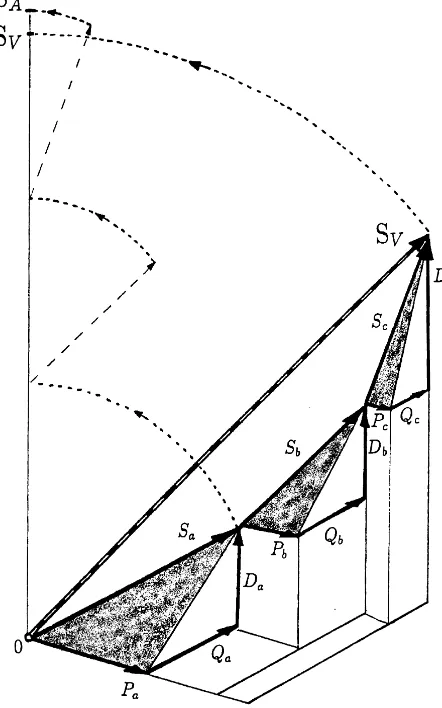
This expression stems from the power triangle, S, P, Q, and is useful in power flow studies. Figure 1 summa-rizes the conventional power flow directions as interpreted in literature (Stevens [B12]4).

3.1.2 Single-Phase nonsinusoidal

For steady-state conditions a nonsinusoidal instantaneous voltage or current has two distinctive components: the power system frequency components v₁ and i₁, and the remaining terms v_H and i_H that contains all inte-ger and noninteinte-ger number harmonics.

4_{The numbers in brackets correspond to those of the bibliography in Annex C.} S

|| = VI

S = P2+Q2

2f = 2ω⁄2π

P_F

|| P

S ---=

S = V I∗ = P+ jQ

V = V∠0°

I∗ = I∠θ

v₁ = 2V₁sin(ωt–α₁)

i₁ = 2I₁sin(ωt–β₁)

v_H 2 V_hsin(hωt–αh) h

∑

≠1

=

i_H 2 I_hsin(hωt–β_h)

h

∑

≠1

The corresponding rms values squared are as follows:

where

=

=

NOTE—The direct voltage and the direct current terms V₀ and I₀, obtained for h = 0, must be included in V_H and I_H.

They correspond to a hypothetical ; . Significant

dc components are rarely present in ac power systems; however, traces of dc are not uncommon.

Figure 1—Four-quadrant power flow directions (see [B12])

Copyright  1983 IEEE

V2 1 kT

--- v2dt τ τ+kT

∫

V₁2+V_H2

= =

I2 1 kT

--- i2dt τ τ+kT

∫

I₁2+I_H2

= =

V_H2 V_h2

h

∑

≠1

V2–V₁2

= ||

I_H2 I_h2

h

∑

≠1

I2–I₁2

= ||

3.1.2.1 Total harmonic distortion

The overall deviation of a distorted wave from its fundamental can be estimated with the help of the total harmonic distortion. The total harmonic distortion of the voltage is as follows:

The total harmonic distortion of the current is as follows:

3.1.2.2 Instantaneous power (W)

where

p_a =

is a term that contains all the components that have non-zero average value, and

is a term that does not contribute to the net transfer of energy, i.e., its average value is nil.

The angle is the phase angle between the phasors V_h and I_h.

3.1.2.3 Active power (W)

3.1.2.4 Fundamental or 60 Hz active power (W)

3.1.2.5 Harmonic active power (W)

NOTE—For ac motors, which make up the vast majority of loads, the harmonic active power is not a useful power. Con-sequently, it is useful to separate the fundamental active power P₁ from the harmonic active power P_H.

TH D_v

|| VH

V₁

--- V V₁

--- 

 2_–1

= =

TH D_I

|| IH

I₁

--- I I₁

----   2_–1

= =

p = vi

p = p_a+p_q

V_hI_hcosθh[1–cos(2hωt)] h

∑

p_q V_hI_h θh (2hωt) 2VmInsin(mωt+αm)sin(nωt+βn) m≠n

m n, ≠1

∑

+ sin sin h

∑

=

θh = βh–αh

P || 1

kT

--- p td τ τ+kT

∫

=

P = P₁+P_H

P₁

|| 1

kT

--- v₁i₁dt τ

τ+kT

∫

V₁I₁cosθ₁

= =

P_H V_hI_hcosθh h

∑

≠1

P–P₁||

3.1.2.6 Fundamental reactive power (var)

3.1.2.7 Budeanu’s reactive power (var)

where

Q_BH =

NOTE—The usefulness of Q_B for quantifying the flow of harmonic nonactive power has been questioned by many engi-neers (Czarnecki [B2], Lyon [B10]). Field measurements and simulations (Pretorius, van Wyk, and Swart [B11]) prove that in many situations Q_BH < 0, thus leading to situations where Q_B < Q₁.

3.1.2.8 Apparent power (VA)

NOTE—An important practical property of S is that the power loss ∆P, in the feeder that supplies the apparent power S,

is a nearly linear function of S2 (Emanuel[B4]).

where

R is an equivalent shunt resistance, representing transformer core losses and cable dielectric losses, r_e is the effective Thevenin resistance. Theoretically r_e can be obtained from the equivalence of losses

as follows:

where

K_sh is the skin effect coefficient for the h harmonic, r_dc is the Thevenin dc resistance (Ω).

Q₁ || ω1

kT

--- i₁[

∫

v₁dt]dt τ

τ+kT

∫

=

V₁I₁sinθ₁

=

Q_B V_hI_hsinθh h

∑

=

QB = Q1+QBH

V_hI_hsinθh h

∑

≠1

S || = VI

∆P re V2 ---S2 V

2

R ---+ =

r_eI2 r_dc K_shI_h2

h

3.1.2.9 Fundamental or 60/50 Hz apparent power (VA)

Fundamental apparent power S₁ and its components P₁ and Q₁ are the actual quantities that help define the rate of flow of the electromagnetic field energy associated with the 60/50 Hz voltage and current. This is a product of high interest for both the utility and the end-user.

3.1.2.10 Nonfundamental apparent power (VA)

The separation of the rms current and voltage into fundamental and harmonic terms (see 3.1.2) resolves the apparent power in the following manner (Emanuel [B5]):

is the nonfundamental apparent power, and is resolved in the following three distinctive terms:

3.1.2.11 Current distortion power (var)

3.1.2.12 Voltage distortion power (var)

3.1.2.13 Harmonic apparent power (VA)

3.1.2.14 Harmonic distortion Power (var)

NOTE—In practical power systems, THD_V < THD_I and S_N can be computed using the following expression (Emanuel [B5]):

When THD_V≤ 5% and THD_I≤ 200%, this expression yields an error less than 0.15%.

S₁

|| = V₁I₁

S₁2 = P₁2+Q₁2

S2 = (VI)2 = (V2₁+V_H2)(I₁2+I_H2) = (V₁I₁)2+(V₁I_H)2+(V_HI₁)2+(V_HI_H)2= (S₁2+S2_N)

S_N

|| = S2–S₁2

S_N2 = D₁2+D_v2+S_H2

D_I = V₁I_H = S₁(TH D_I) ||

D_v = V_HI₁ = S₁(TH D_V) ||

S_H = V_HI_H = S₁(TH D₁)(TH D_V) ||

S_H = P_H2 +D_H2

D_H

|| = S_H2 –P_H2

For THD_V < 5% and THD_I > 40%, an error less than 1.00% is obtained using the following expression (Emanuel [B5]):

3.1.2.15 Nonactive power (var)

This power lumps together both fundamental and nonfundamental nonactive components. In the past, this power was called fictitious power.

3.1.2.16 Budeanu’s distortion power (var)

This power results from the resolution of S using Budeanu’s reactive power Q_B (see 3.1.2.7) that leads to the following:

hence,

NOTE—This distortion power is affected by the deficiency of Q_B (Pretorius, van Wyk, and Swart [B11]).

3.1.2.17 Fundamental or 60/50 Hz power factor

This ratio helps evaluate separately the fundamental power flow conditions. It can be called the fundamental power factor or 60/50 Hz power factor. It is also often referred to as the displacement power factor.

3.1.2.18 Power factor

NOTES

1—The apparent power S can be viewed as the maximum active power that can be transmitted to a load while keeping its load voltage V constant and line losses constant. The result is that for a given S and V, maximum utilization of the line is obtained when P = S; hence, the ratio P/S is a utilization factor indicator.

2—The overall degree of harmonic injection produced by a large nonlinear load, or by a group of loads or consumers, can be estimated from the ratio S_N /S₁. The effectiveness of harmonic filters also can be evaluated from such a measure-ment. The measurements of S₁, P₁, P_F1, or Q₁ help establish the characteristics of the fundamental power flow.

S_N≈S₁(TH D_I)

N

|| = S2–P2

S2 = P2+Q_B2+D_B2

D_B = S2–P2–Q_B2

P_F1 cosθ₁ P1

S₁ ---||

= =

P_F

|| P

S ---=

P_F P S

--- P1+PH S₁2+S_N2

--- (P1⁄S1)[1+(PH⁄P1)] 1+(S_N⁄S₁)2

---= = = [1+(PH⁄P1)]PF1

3—In most common practical situations, . It is difficult to measure correctly the higher-order components of

P_H with most metering instrumentation. Thus, one cannot rely on measurements of P_H components when making tech-nical decisions regarding harmonics compensation, energy tariffs, or to quantify the detrimental effects made by a nonlinear or parametric load to a particular power system (Emanuel [B5]; IEEE [B9]; Swart, van Wyk, and Case [B13]).

4—When THD_V< 5% and THD_I > 40%, it is convenient to use the following expression:

5— In typical nonsinusoidal situations, D_I > D_V > S_H > P_H.

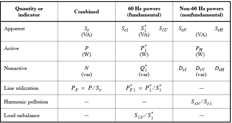
The definitions presented in 3.1.2.8 to 3.1.2.17 are summarized in Table 1.

3.2 Three-Phase systems

3.2.1 Three-Phase sinusoidal balanced

In this case, the line-to-neutral voltages are as follows:

Table 1—Summary and grouping of the quantities in single-phase systems with nonsinusoidal waveforms

Quantity or

indicator Combined

60 Hz powers (fundamental)

Non-60 Hz powers (nonfundamental)

Apparent S

(VA)

S₁

(VA)

S_N

(VA)

S_H

(VA)

Active P

(W)

P₁

(W)

P_H

(W)

Nonactive N

(var)

Q₁

(var)

D_I D_V

(var)

D_H

Line utilization P_F = P/S P_F1 = P₁/S₁ —

Harmonic pollution — — S_N /S₁

P_H«P₁

P_F 1

1+TH D_I2 ---P_F1

≈

v_a = 2V_lnsin(ωt)

v_b = 2V_lnsin(ωt–120°)

The line currents have similar expressions. They are as follows:

NOTES

1—Perfectly sinusoidal and balanced three-phase, low-voltage systems are uncommon. Only under laboratory condi-tions, using low distortion power amplifiers, is it possible to work with ac power sources with THD_V < 0.1% and voltage unbalance V –/V + < 0.1%. Practical low-voltage systems will rarely operate with THD_V < 1% and V –/V + < 0.4%, where

V + and V – are the positive- and negative-sequence voltages, see 3.2.2.2.1.

2— In the case of a three-wire system, the line-to-neutral voltages are defined assuming an artificial neutral node.

3.2.1.1 Instantaneous power (W)

3.2.1.2 Active power (W)

where

is line-to neutral voltage,

is line-to-line voltage.

3.2.1.3 Reactive power (var)

3.2.1.4 Apparent power (VA)

3.2.1.5 Power factor i_a = 2Isin(ωt–θ)

i_b = 2Isin(ωt–θ–120°)

i_c = 2Isin(ωt–θ+120°)

p

|| = v_ai_a+v_bi_b+v_ci_c = P

P || 1

kT

--- p td τ τ+kT

∫

=

P = 3V_lnIcosθ = 3V_llIcosθ

V_ln

V_ll

Q = 3V_lnIsinθ = 3V_llIsinθ

Q = S2–P2||

S= 3V_lnI

|| = 3V_llI

P_F

|| P

3.2.2 Three-Phase sinusoidal unbalanced

In this case, the three current phasors, I_a, I_b, and I_c, do not have equal magnitudes, nor are they shifted exactly with respect to each other. Load unbalance leads to asymmetrical currents that in turn can cause volt-age asymmetry. There are situations when the three voltvolt-age phasors are not symmetrical. This leads to asymmetrical currents even when the load is perfectly balanced.

The line-to-neutral voltages are as follows:

The line currents have similar expressions. They are as follows:

NOTE—In the case of three-wire systems, the line-to-neutral voltages are de_fined assuming an arti_ficial neutral node, which can be obtained with the help of three identical resistances connected in Y.

3.2.2.1 Instantaneous power (W)

for three-wire systems where , and

where v_ab, v_bc, and v_ca are the instantaneous line-to-line voltages.

3.2.2.2 Active power (W)

where

v_a = 2V_alnsin(ωt+αa)

v_b = 2V_blnsin(ωt+αb–120°)

v_c = 2V_clnsin(ωt+αc+120°)

i_a = 2I_asin(ωt–βa)

i_b = 2I_bsin(ωt–βb–120°)

i_c = 2I_csin(ωt–βc+120°)

p

|| = v_ai_a+v_bi_b+v_ci_c

i_a+i_b+i_c = 0

p

|| = v_abi_a+v_cbi_c = v_aci_a+v_bci_b = v_bai_b+v_cai_c

P || I

kT

--- p td τ τ+kT

∫

=

P

|| = P_a+P_b+P_c

P_a 1 Kt

--- v_ai_adt τ

τ+kT

∫

V_alnI_acosθa; θ a αa+βa

P_a, P_b, and P_c are phase active powers.

3.2.2.2.1 Positive-, negative-, and zero-sequence active powers (W)

In some situations the use of symmetrical components may be helpful. The symmetrical voltage components V+, V–, V0 and current components I+, I–, I0 with the respective phase angles θ+_{, θ}–_{, θ}0_{yield the following}

three active power components:

The positive-sequence active power

The negative-sequence active power

The zero-sequence active power

The total active power is

3.2.2.3 Reactive power (var)

Per phase reactive powers are defined with the help of the following expressions:

For the vector apparent power S_V (see 3.2.2.6) the total reactive power Q is as follows:

NOTE—The above expression of Q cannot be used in conjunction with the arithmetic apparent power S_A, defined in 3.2.2.5.

P_b 1 Kt

--- v_bi_bdt τ

τ+kT

∫

V_blnI_bcosθb; θ b αb+βb

= = =

P_c 1 Kt

--- v_ci_cdt τ

τ+kT

∫

V_clnI_ccosθc; θ c αc+βc

= = =

P+ = 3V_l+_nI+cosθ+

P– = 3V_l–_nI–cosθ–

P0 = 3V_l0_nI0cosθ0

P = P++P–+P0

Q_a ω kT

--- i_a[

∫

v_adt]dt τ

τ+kT

∫

V_alnI_asinθ_a

= =

Q_b ω kT

--- i_b[

∫

v_bdt]dt τ

τ+kT

∫

V_blnI_bsinθb

= =

Q_c ω kT

--- i_c[

∫

v_cdt]dt τ

τ+kT

∫

V_clnI_csinθc

= =

3.2.2.3.1 Positive-, negative-, and zero-sequence reactive powers (var)

In some situations the use of symmetrical components may be helpful. The three reactive powers are as follows:

The positive-sequence reactive power

The negative-sequence reactive power

The zero-sequence reactive power

The total reactive power is

3.2.2.4 Phase apparent powers (VA)

; ;

;

3.2.2.5 Arithmetic apparent power (VA)

NOTE—The arithmetic apparent power cannot be resolved according to 3.1.1.4,

where

P =

Q =

Q+ = 3V_l+_nI+sinθ+

Q– = 3V_l–_nI–sinθ–

Q0 = 3V_l0_nI0sinθ0

Q = Q++Q–+Q0

S_a = V_alnI_a S_b = V_blnI_b S_c = V_clnI_c

S_a2 = P_a2+Q_a2 S_b2 = P2_b+Q_b2 S_c2 = P_c2+Q_c2

S_A = S_a+S_b+S_c

S_A≠ P2+Q2

P_a+P_b+P_c

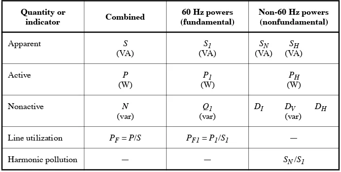
3.2.2.6 Vector apparent power (VA)

A geometrical interpretation of S_V is presented in Figure 2.

3.2.2.6.1 Positive-, negative-, and zero-sequence apparent powers (VA) S_V = P2+Q2

S_V = P_a+P_b+P_c+ j Q( _a+Q_b+Q_c) = P+ jQ

S_V = P++P–+P0+ j Q( ++Q–+Q0)

Figure 2—Arithmetic and vector apparent powers: sinusoidal situation

S

A

S

c

S+ ₌ S+ _{= P}+_{+ jQ}+

S– = S– = P–+ jQ–

S0 = S0 = P0+ jQ0

S_{V =} S+₊S–₊S0

3.2.2.7 Vector power factor and arithmetic power factor

NOTE—A three-phase line supplying one or more customers should be viewed as one single path, one entity that trans-mits the electric energy to locations where it is converted into other forms of energy. It is wrong to view each phase as an independent energy route. In poly-phase systems, the meaning of power factor as a utilization indicator is retained (see 3.1.2.18). Unity power factor means minimum possible line losses for a given total active power transmitted. The follow-ing example helps clarify certain limitations pertinent to the old apparent power definitions S_A and S_V .

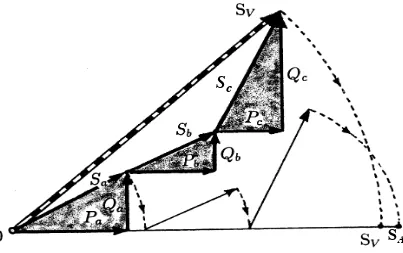
EXAMPLE:

A four-wire, three-phase system, Figure 3(a), supplies a resistance R connected between phases a and b. The active power dissipated by R is as follows:

and assume each line has the resistance r that results in a line current , which is causing the following power loss:

Now let us assume a second system with a perfectly balanced three-phase load, Figure 3(b), consisting of three resistances R_B connected in Y. This system dissipates the same power as the unbalanced one; hence,

R_B = R results, and the line power loss for the balanced system is as follows: P_FV P

S_V ---=

PFA P SA ---=

P_R 3Vln 2

R ---=

I = 3V_ln⁄R

∆P 6r Vln R

--- 

 2

=

P_RB 3Vln

2

R_B --- P_R

= =

∆P_B 3r Vln R

--- 

 2 _0.5∆P

= =

The power loss dissipated in the unbalanced system is twice the power loss in the balanced one. This obser-vation leads to the conclusion that the unbalanced system has . The balanced system operates with minimum possible losses for a given load voltage and active power, hence its power factor is unity.

For the unbalanced system, the arithmetic and vector apparent powers have the following components [see phasor diagram in Figure 3(c)]:

;

; ;

The total active power is

The total reactive power is

The vector apparent power is

The arithmetic apparent power is

The power factor computed for the unbalanced system using S_V gives . The power fac-tor computed with S_A gives .

If the unbalanced load consists of a resistance connected between line and neutral, then and .

These results indicate that both the arithmetic and the vector apparent powers do not measure or compute power factor correctly for unbalanced loads. As a rule, .

3.2.2.8 Effective apparent power (VA)

This concept assumes a virtual balanced circuit that has exactly the same power losses as the actual unbalanced circuit. This equivalence leads to the definition of an effective line current I_e and an effective line-to-neutral voltage V_e (Depenbrock [B3], Emanuel [B5]).

P_F<1

P_a V_aI_acos(30°) 3 2 ---V_lnI

= = Q_a V_aI_asin30° 1

2 ---V_lnI

= = S_a = V_aI_a = V_lnI

P_b V_bI_bcos(–30°) 3 2 ---V_lnI

= = Q_b V_bI_bsin(–30°) –1 2 ---V_lnI

= = S_b = V_bI_b = V_lnI

P_c = Q_c = S_c = 0

P P_a+P_b 3V_lnI 3Vln 2

R

---= = =

Q = Q_a+Q_b+Q_c = 0

S_V = P

S_A S_a+S_b+S_c 2V_lnI 2 3Vln

2

R

---= = =

PFV = P S⁄ V = 1.0 PFA = P S⁄ A = 3 2⁄ = 0.866

S_a = S_b = P P_FA = P_FV = 1.0

For a four-wire system, the balance of power loss is expressed in the following way:

where

I_n is the neutral rms current

r is the line resistance assumed to be equal to the neutral wire (or return path) resistance,

R is the equivalent neutral shunt resistance, also assumed to be 1/3 of the equivalent line-to-line shunt resistance.

From the above equations, the equivalent current and voltage for a four-wire system is obtained.

and

For practical situations where the differences between α_a, α_b, and α_c do not exceed ±10° and the differences among the line-to-neutral voltages remain within the range of ±10%, the following simplified expression can be used:

The error caused by this simplified expression is less than 0.2% for the above conditions.

In the same manner, the equivalent current and voltage for a three-wire system can be found by using

From these equations, the following results:

and

r I( 2_a+I_b2+I_c2+I2_n) = 3r I_e2

V_a2+V_b2+V_c2 R

--- Vab

2

V_bc2 V_ca2

+ +

3R

---+ 3Ve

2

R --- 9Ve

2 3R ---+ = I_e || Ia

2

I_b2 I_c2 I_n2 + + +

3

--- ( )I+ 2+( )I– 2+4( )I0 2

= =

V_e 1 18

--- 3[ (V_a2+V_b2+V_c2)+V2_ab+V_bc2 +V_ca2 ]

|| (V+)2 (V–)2 V

0

( )2 2

---+ +

=

V_e Vab 2

V_bc2 V_ca2

+ +

9

---≈

|| = (V+)2+(V–)2

r I( _a2+I2_b+I_c2) = 3r I_e2

V_ab2 +V_bc2 +V_ca2 3R

--- 9Ve

2

3R ---=

I_e

|| Ia 2

I_b2 I_c2 + +

( )

3

--- ( )I+ 2+( )I– 2

= =

V_e

|| Vab 2

V_bc2 V_ca2

+ +

9

--- (V+)2+(V–)2

The effective apparent power (Buchholz [B1], Goodhue [B7]) is as follows:

3.2.2.9 Effective power factor

NOTES

1—Applying the concept of S_e to the unbalanced circuit described in the example given in 3.2.2.7, results in the following:

;

;

Hence the power factor is as follows:

2—When the system is balanced, then

and

3—When the system is unbalanced, then

and

4—Both the vector and the arithmetic apparent powers do not satisfy the linearity requirement of system power loss ver-sus the apparent power squared (Emanuel [B4]).

S_e

|| = 3V_eI_e

P_Fe

|| = P S⁄ _e

V_e = V_ln I_e Ia 2

I_b2 + 3

--- 2Vln R

---= =

S_e 3 2Vln

2

R

---= P 3Vln

2

R ---=

P_Fe P S_e --- 1

2

--- 0.707<P_FA<P_FV

= = =

V_a = V_b = V_c = V_ln = V_e

I_a = I_b = I_c = I

I_n = 0

S_V = S_A = S_e

S_V≤S_A≤S_e

3.2.2.10 Positive-Sequence power factor

This index has the same significance as the fundamental power factor P_F1 (see 3.1.2.17). It helps evaluate the positive-sequence power flow conditions.

3.2.2.11 Effective apparent power resolution for three-phase unbalanced sinusoidal systems

where

3.2.2.12 Unbalance power

evaluates the unbalance of the system. It should not be confused with the voltage unbal-ance. It reflects both the load unbalance and voltage asymmetry.

3.2.3 Three-Phase nonsinusoidal balanced systems

The line-to-neutral voltages are as follows:

The line currents have similar expressions. They are as follows: P_F+

|| = P+⁄S+

S_e2 = (S+)2+(S_U)2

S+ = 3V_l+_nI+

S+

( )2 = (P+)2+(Q+)2

S_U = S_e2–(S+)2

va 2V1 ωt 2 Vhsin(hωt+αh) h

∑

≠1

+ sin =

v_b 2V₁ (ωt–120°) 2 V_hsin(hωt+αh–120°h) h

∑

≠1

+ sin

=

v_c 2V₁ (ωt+120°) 2 V_hsin(hωt+αh+120°h) h

∑

≠1

+ sin

=

i_a 2I₁ (ωt+β₁) 2 I_hsin(hωt–βh) h

∑

≠1

+ sin

=

i_b 2I₁ (ωt+β₁–120°) 2 I_hsin(hωt–βh–120°h) h

∑

≠1

+ sin

=

i_c 2I₁ (ωt+β₁+120°) 2 I_hsin(hωt–βh+120°h) h

∑

≠1

+ sin

NOTES

1—In this case, S_a = S_b= S_c, P_a = P_b = P_c, Q_Ba = Q_Bb = Q_Bc, and D_a = D_b = D_c.

2—When triplen harmonics are present, in spite of the fact that the load is perfectly balanced, the neutral current is not nil.

The above equation illustrates the fact that such a system has the potential to produce significant additional power loss in the neutral wire and ground path. This situation should be reflected in the P_F expression.

3—The positive-sequence triplen harmonic voltages that contribute to the rms value of cancel each other and do not appear in :

This means that

The expression yields an error less than 0.33% when the rms value of all the triplen harmonics voltage is

These observations lead to the conclusion that for three-phase systems with nonsinusoidal wave forms the effective apparent power S_e and its components offer an improved set of definitions to better evaluate the power flow conditions (see 3.2.3.2).

3.2.3.1 Apparent power with Budeanu’s Resolution

where

is the active power (W)

where

i_n i_a+i_b+i_c 3 2I_hsin(hωt–βh) h=0 3 6, , ,

∑

…

= =

I_n I_h2

h=0 3 6

∑

, , ,…

=

V_ln V_ll

v_ab v_a–v_b 3 2V₁ (ωt+30°) 3 2 V_hsin(hωt+αh+30°h) h≠0 3 6 9, , , ,

∑

…

+ sin

= =

3V_llI≤3V_lnI

S≈ 3V_llI

V_h2

h=0 3 6

∑

, , ,…

0.08V_ln <

S = 3V_lnI = P2+Q2_B+D_B2

P = P₁+P_H

P₁ = 3V₁I₁cosβ₁

P_H 3 V_hI_hcosθh h

∑

≠1

=

is the Budeanu’s reactive power (var)

where

is the Budeanu’s distortion power (var).

The reactive power Q_B has a drawback that is explained in 3.1.2.7.

3.2.3.2 Effective apparent power (VA)

For a four-wire balanced system,

and

For a three-wire system,

and

NOTE—In a four-wire system, the apparent power and .

The detailed resolution of S_e into practical components is presented in 3.2.4.3.

3.2.4 Three-Phase nonsinusoidal and unbalanced systems

This subclause covers the most general case. It deals with all the situations presented in the previous clauses. Q_B = Q₁+Q_BH

Q₁ = 3V₁I₁sin(–β₁)

Q_H 3 V_hI_hsinθh h

∑

≠1

=

D_B = S2–P2–Q_B2

S_e

|| = 3V_eI_e

V_e = V_ln

I_e 3I 2

I_n2 + 3

--- I2 I_h2

h=0 3 6

∑

, , ,…

+

= =

V_e = V_ll⁄ 3

I_e = I

S_e = S = 3V_llI

3.2.4.1 Arithmetic apparent power (with Budeanu’s Resolution) (VA)

This definition is an extension of Budeanu’s apparent power resolution for single-phase systems. For each phase, a per phase apparent power is identifiable as follows:

From the above equations, the following arithmetic apparent power is obtained:

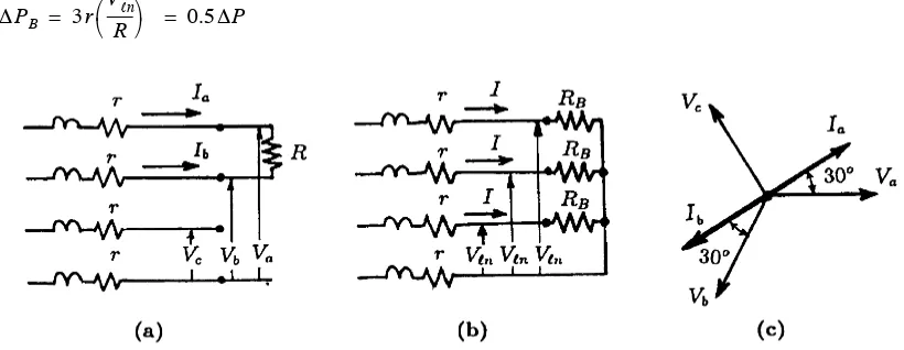
NOTE—The power factor maintains the significance previously explained. However the major draw-back of this definition stems from the difference between the quantities

and (see Figure 4).

S_a = P_a2+Q_Ba2 +D_Ba2

S_b = P_b2+Q_Bb2 +D_Bb2

S_c = P_c2+Q_Bc2 +D_Bc2

S_A = S_a+S_b+S_c

PFA = P S⁄ A

Q_Ba+Q_Bb+Q_Bc

[ ]2+[D_Ba+D_Bb+D_Bc]2 S_A2–P2

Figure 4—Arithmetic S_A, and Vector S_V , apparent powers: unbalanced nonsinusoidal conditions

3.2.4.2 Vector apparent power (VA), with Budeanu’s Resolution

Using the same notations as in 3.2.4.1 applied to 3.2.2.5 results in the following:

where

NOTE—While this expression is free of the drawback discussed in the previous note, the problems with the Budeanu’s reactive power also affect this apparent power resolution. Moreover, the fact that no flow direction can be assigned to D_B, limits the usefulness of this definition even more.

3.2.4.3 The effective apparent power and its resolution

In the past, S_e was divided into active power P and nonactive power N as follows:

This approach, however, does not separate out the positive-sequence fundamental powers. The approach used in 3.1.2.8 to 3.1.2.14 and 3.2.2.8 can be expanded for this situation. The rms effective current and volt-age are divided into two components—the fundamental and the nonfundamental (Emanuel [B5], IEEE [B9]).

where for a four-wire system: S_V = P2+Q_B2+D_B2

P = P_a+P_b+P_c

Q_B = Q_Ba+Q_Bb+Q_Bc

D_B = D_Ba+D_Bb+D_Bc

S_e2 = P2+N2

I_e = I_e2₁+I_eH2

V_e = V_e2₁+V_eH2

I_e || Ia

2

I_b2 I_c2 I_n2 + + +

3 ---=

I_e1

|| Ia1 2

I_b2₁ I_c2₁ I_n2₁

+ + +

3

---=

I_eH IaH 2

I_bH2 I_cH2 I_nH2

+ + +

3

--- I_e2+I_e2₁||

= =

V_e

|| 1

18

For three-wire systems, and the expressions become simpler.

The resolution of is implemented in the manner shown in 3.1.2.8 to 3.1.2.14.

where

is the fundamental effective apparent power,

S_eN is the nonfundamental effective apparent power. The resolution of S_eN is identical to the resolution of S_N given in 3.1.2.10.

V_e1

|| 1

18

--- 3[ (V_a2₁+V_b2₁+V2_c1)+V_ab2 ₁+V_bc2 ₁+V_ca2 ₁] =

V_eH 1 18

--- 3[ (V_aH2 +V2_bH+V_cH2 )+V_abH2 +V_bcH2 +V2_caH] V_e2–V_e2₁||

= =

I_n1 = I_nH = 0

I_e || Ia

2

I_b2 I_c2 + +

3 ---=

I_e1

|| Ia1 2

I_b2₁ I_c2₁ + +

3 ---=

I_eH IaH 2

I_bH2 I_cH2

+ +

3

--- I_e2+I_e2₁||

= =

V_e

|| Vab 2

V_bc2 V_ca2

+ +

9 ---=

V_e1

|| Vab1 2

V_bc2 ₁ V_ca2 ₁

+ +

9

---=

V_eH VabH 2

V_bcH2 V_caH2

+ +

9

--- V_e2–V_e2₁||

= =

S_e = 3V_eI_e

S_e2 = S_e2₁+S_eN2

S_e1

|| = 3V_e1I_e1

The current distortion power, voltage distortion power, and harmonic apparent power are as follows:

and

By defining the equivalent total harmonic distortions as follows:

practical expressions, identical to those found in 3.1.2.10 through 3.1.2.14, for the nonfundamental apparent power S_eN and its components D_eI , D_eV , and S_eH are obtained.

For systems with and , the following approximation is recommended [B9]:

The load unbalance can be evaluated using the following fundamental unbalanced power:

where

is the fundamental positive-sequence apparent power (VA). This important apparent power con-tains the following components:

is the fundamental active power (W), and

is the fundamental reactive power (var). D_e1

|| = 3V_e1I_eH

D_eV

|| = 3V_eHI_e1

S_eH

|| = 3V_eHI_eH

D_eH

|| = S_eH2 –P_eH2

TH D_eV

|| VeH

V_e1 ---=

TH D_eI

|| IeH

I_e1 ---=

S_eN = S_e1 TH D_eI2 +TH D2_eV+(TH D_eITH D_eV)2

D_eI = S_e1(TH D_I)

D_eV = S_e1(TH D_V)

S_eH = S_e1(TH D_I)(TH D_V)

TH D_eV≤5% TH D_eI≥40%

S_eN≈S_e1(TH D_eI)

S_U1 = S_e2₁–(S₁+)2

S₁+

P₁+ = 3V₁+I₁+cosθ₁+

Together they result in

and the fundamental or the 60/50 Hz positive-sequence power factor

that plays the same significant role that the fundamental power factor has in nonsinusoidal single-phase systems.

The power factor is

The most important definitions are summarized in Table 2.

This table lists the three basic powers: apparent, active, and nonactive. The columns are partitioned into three groups—the combined powers, the 60 Hz powers (fundamental powers), and the non-60 Hz powers (nonfundamental powers). The last three rows give the indices: power factors (i.e., line utilization factor), harmonic pollution factor, and load unbalance factor.

Table 2—Summary and grouping of quantities for three-phase systems with nonsinusoidal waveforms

Quantity or

indicator Combined

60 Hz powers (fundamental)

Non-60 Hz powers (nonfundamental)

Apparent S_e

(VA)

S_e1

(VA)

S_1U S_eN

(VA)

S_eH

Active P

(W) (W)

P_H

(W)

Nonactive N

(var) (var)

D_eI D_eV

(var)

D_eH

Line utilization —

Harmonic pollution — —

Load unbalance — —

S₁+ = (P₁+)2+(Q₁+)2

P_F+₁ || P1

+

S₁+ ---=

P_F

|| P

S_e ---=

S₁+

P₁+

Q₁+

P_F = P S⁄ _e P+_F1 = P₁+⁄S₁+

S_eN⁄S_e1

Annex A

(informative)

Theoretical examples

A.1 Single-Phase nonsinusoidal

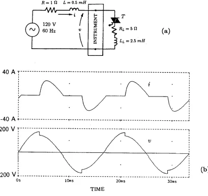
The circuit used for this example is presented in Figure A.1(a). Voltage v and current i waveforms are pre-sented in Figure A.1(b). Normalized harmonic voltages and currents are summarized in Table A.1.

Figure A.1—Single-Phase circuit with thyristorized load (a) Circuit diagram

The values of the rms, fundamental, and total harmonic voltage and current are as follows:

The total harmonic distortions of voltage and current are as follows:

Computations lead to the results summarized in Table A.2.

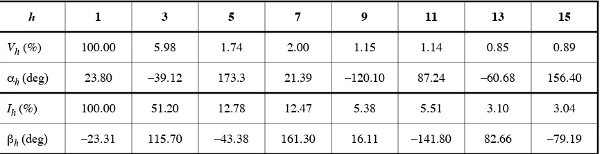
Table A.1—Percent Harmonic Voltage and Current Phasors. Base Values: V₁ = 111.09 V; I₁ = 11.17 A

h 1 3 5 7 9 11 13 15

V_h(%) 100.00 5.98 1.74 2.00 1.15 1.14 0.85 0.89

αh(deg) 23.80 –39.12 173.3 21.39 –120.10 87.24 –60.68 156.40

I_h (%) 100.00 51.20 12.78 12.47 5.38 5.51 3.10 3.04

βh (deg) –23.31 115.70 –43.38 161.30 16.11 –141.80 82.66 –79.19

Table A.2—Percent powers Base value: S1 = 1229.70 VA

S_e = 114.41 S₁ = 100.00 S_N = 55.59

S_H = 3.80

P = 66.35 P₁ = 69.61 P_H = –3.26

N = 93.20 Q₁ = 73.07 D_I= 55.06

D_V = 6.91

D_H = 1.96

Q_B = 71.58 D_B = 59.69

V = 110.35 V

V₁ = 110.09 V

V_H = 7.55 V

I = 12.75 A

I₁ = 11.17 A

I_H = 6.15 A

TH D_V = 0.069

TH D_I = 0.549

The nonlinear load is supplied with a 60 Hz active power , and oper-ates with a power factor P_F = 0.580 and a fundamental factor . A small part of the 60 Hz active power is converted by the triac into harmonic power (returned to the power system) as follows:

The fundamental current lags the fundamental voltage by an angle , yield-ing a 60 Hz reactive power as follows:

Budeanu’s reactive power , is smaller than Q₁.

The degree of distortion can be estimated with the ratio , which is nearly equal to .

The overall amount of harmonic pollution is quantified with the help of the non-60 Hz apparent power as follows:

This value is nearly equal to the current distortion power . The small difference is due to the voltage distortion power and the harmonic apparent power .

The fundamental apparent power S₁ and its components P₁ and Q₁ make up the bulk of the apparent power S. Nevertheless, in this particular example, the nonfundamental apparent power S_N represents a significant amount of the total apparent power.

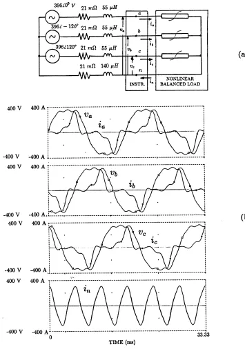
A.2 Three-Phase balanced nonsinusoidal system

The circuit is shown in Figure A.2. In this example, the third and the ninth harmonic currents are zero-sequence components and cause a large neutral current, which results in additional energy loss in the neutral conductor. Harmonic phasors obtained from this circuit simulation are summarized in Table A.3. Voltage and current components of higher interest have the following rms and total harmonic distortion values:

; ; ;

; ; ;

; ; ;

; ;

The neutral current has no 60 Hz, 300 Hz, or 420 Hz components (i.e., neither positive nor negative sequence components). The line-to-line voltage, however, lacks the 180 Hz and the 540 Hz components (zero-sequence). This situation is reflected in the following apparent power computations:

A 0.94% difference between these two values is observed.

P₁ = 0.6961×1229.7 = 856.04 W P_F1 = cosθ₁ = 0.696

P_H = –0.0326×1229.70 = –40.1 W

θ₁ = 23.80°+23.31° = 47.11°

Q₁ = 0.7307×1229.7 = 898.61 var

Q_B = 880.22 var

S_N⁄S₁ = 0.556 TH D_I = 0.549

S_N = 0.556×1229.70 = 683.63 VA

D₁ = 677.05 var

D_V = 84.97 var S_H = 46.73 VA

V_a = 279.94 V V_a1 = 277.25 V V_aH = 38.70 V TH D_Va = 0.139

V_ab = 480.29 V V_ab1 = 480.20 V V_abH = 9.55 V TH D_Vab = 0.020

I_a = 129.40 A I_a1 = 99.58 A I_aH = 82.25 A TH D_Ia = 0.823

I_n = 207.20 A I_n1 = 0 A I_nH = 207.20 A

3VlnIa = 3×279.94×129.4 = 108.673 kVA

Figure A.2—Three-Phase, four-wire circuit with a nonlinear balanced load (a) Circuit diagram

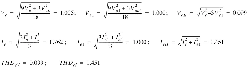
The normalized equivalent voltages and currents are a