Volume 26, Number 3, 2011, 310 – 324
THE IDENTIFICATION OF STRUCTURAL BREAK AT TIME
SERIES DATA ON INDONESIAN ECONOMY 1990Q1-2008Q4:
THE APPLICATION OF ZIVOT AND
ANDREWS’ EXPERIMENT
Rahman Dano Mustafa Universitas Khairun Ternate
ABSTRACT
Before the 1997/1998 economic crisis that enhanced the fluctuation of some Indonesian macroeconomic indicators, Indonesian economic indicators seemed to run quite well as to make it attractive as business destination. The economic turbulence has brought about the enhancement of its macroeconomic indicators fluctuation: the depreciation of Indonesian Rupiah’s exchange rate, the sharp contraction of GDP, the ever-increasing inflation pressure, and the interest rate hike.
The objective of this paper is to identify the right timing of the major structural break on Indonesian economy through the application of Zivot and Andrew’s procedure (ZA) (Zivot and Andrews, 1992), with time series data in the period of Q1 1990-Q4 2008. The ZA model empirical test outcome shows that endogenously the significance of structural break for most macroeconomic variables necessitates at least one hypothesis of null unit root that can be rejected for most of the investigated variables. The potential structural break in series (ADF-test) also allows some originally non-stationary-unit contained variables to turn into a stationary ones. These results are statistically significant as the endogenously appropriate break (ZA-test) coexisted with the Indonesian financial-crisis shocks in 1997/1998.
Keywords: structural break, unit root test, macroeconomic time series and Indonesian
economy
INTRODUCTION
Until 1997, East Asian countries had been the role model for other developing countries for its high economic growth that reached the level, similar to the developed countries (Krugman and Obstfeld, 2007: 619). This was all indicated through the high interest rate, the depreciation of asset value, and the deprecia-tion of Indonesian currency. The Asian eco-nomic achievement is worth observing be-cause of its fantastic economic performance
before the financial crisis. The GDP growth rate of ASEAN countries (Indonesia, Malay-sia, the Philippines, Singapore and Thailand) grew annually at an average rate of 8 percent in a period of ten years. Just 30 years before the economic crisis, South Korea’s Gross National Product increased by 10 times, Thailand by 5 times, Malaysia by 4 times (Siswanto, 2007: 156).
world’s attention for its success in develop-ment achievedevelop-ments, one of which can be indicated by the growth of its Real Bruto Domestic Product that reached 6.6% every year in more than three decades (Pincus and Ramli, 2001: 124).
The aim of this paper is to identify the appropriate timing of the major structural break on some macroeconomic variables of Indonesian economy, using data time series of period of 1990Q1–2008Q4, through the appli-cation of Zivot and Andrew’s procedure (ZA) (1992). For adequate comparison, a conven-tional unit root test of Augmented Dickey-Fuller (ADF) and Zivot and Andrew’s procedure (ZA) (1992) were carried out to obtain good result. The structure of this paper consists of five sections. Coming up after this section is section II, which gives a short description of Indonesian economic growth since 1990 until 2008, and the third section contains a short review of referential sources for the unit root test with structural break.
Section IV elaborates the empirical frame-work of unit root applying ZA method to experiment the hypothesis of the unit root of single structural break at unknown point of time. The last, section V serves as a closing.
A SHORT DESCRIPTION OF
INDONESIAN ECONOMY IN 1990 - 2008 Repelita I (Five-year Development Plan I) was introduced in 1969 to give focus on the development of infrastructure for agricultural and rural sector. It is not surprising since almost 30 percent of the rapid economic growth in 1967 - 1973 was contributed by agricultural and rural sector. The achievement of this economic growth is undeniably contributable to the high income from the world oil export, which generated the major economy. In the period of 1973 – 1981, Indonesia was one of those, which gained large benefit out of the world oil hike. (Sharma, 2003: 125).
In the mid-1990s, for more than a decade, manufacturing−which contributed one third of the 1983 - 1995 GDP increase, had become the main machine for Indonesian economic growth. The rapid expansion of manufacturing was not merely fostered by oil and gas-based manufactures, which in 1995, contributed one tenth of the total manufacture output, but also by various manufacturing industries that contributed nine tenth of it. Among others were mostly domestic market-oriented auto-motives manufactures and foreign market oriented manufactures, like wooden and furni-ture, garment, textile, shoes and electronic products. As a result, in the late 1980s, Indo-nesian economy was very much dependent on commerce with a sharply increasing percent-age of the total GDB commerce stream from 14% in 1965 to 54.7% in 1990. This growth had promoted the economic capacity to mobilize saving account, as well-reflected in the increase of national saving in which the percentage of GDP 7.9% in 1965 increased to 26.3% in 1990 (Jomo, 1997 in Sharma, 2003: 125).
capital inflows liberalization (Sharma, 2003: 127, Tjahjono and Anugerah, 2006).
In real sectors, the government attempted to apply expansionary fiscal policy by open-ing domestic market through decreasopen-ing tariff and eliminating negative-listed investment supported by cautious principle-based policy management on macro economy. In this period, such policy had contributed much to the average economic growth of 7.83 percent during 1991 - 1996. Somehow, in the same period, along with the more integrated global market, Indonesia had been trapped in the accumulation of foreign debts that brought about the fragility on Indonesian economy in time of fundamental macroeconomic turbu-lence. Along with the ever-worsening condi-tions of banking, which finally ended up in economic crisis in 1997/1998, Indonesian economy, from then on, tended to grow slower (Tjahjono et al. 2006).
Real GDP grew 8.1 percent each year, at the average, during 1989 - 1996, but slowed down with an average of 5.1 percent during 2002-2006. In term of supply, the contribution of private consumption apparently showed an increasing trend, especially after the year of 2004, after being dominated by net exports and investments that generated the economic growth. While in term of demand, manufac-turing output grew very rapidly after the liberalization of reform in the mid-1980s as such, that it could spur the export demand. However, now Indonesia loses its momentum for its comparative strong point sectors: natural resources (especially timbers, oil and gas) and massive scale activities (textiles, garment and footwear). Electronic goods, including electricity equipment and automo-tive industry have kept growing strongly enough in the post-crisis period. Its consis-tency on promoting private consumption has made the growth of service sector go up very fast in five years of time. This tendency shows an increasingly dynamic non-tradable goods
production sectors, particularly on agriculture, forestry, fishery, mining and manufactures (OECD, 2008; 19).
Despite the economic crisis’ deeper pres-sure, the economic expansion still occurred in 1997 as much as 4.9 percent, still, in 1998, a contraction of economic growth of 13.7 percent took place. For the first quarter in 1999, GDP rose as much as 1.3 percent, the first time since the fourth quarter in 1997, although annually it still showed a contraction of 10.3 percent. The failure of management for the aggregate of demand (demand-side policies) in maintaining the economic stability results in the sharp economic contraction on domestic demand, especially for household consumption and private investment (Bank Indonesia, 2000).
Radelet (1999) stated that between 1990 and the mid-1997, the appreciation of rupiah reached 22 percent (Sharma, 2003; 130). Indonesian rupiah’s exchange rate during the year of 1998 was very fluctuative. In the first quarter, rupiah went through the highest depreciation, reaching Rp16.500 per US dollar in the mid June 1998. For the first half of 1998, the pressure of inflation which took place in October 1998 kept decreasing until its annual inflation rate, once, reached 82.4 percent in September 1998, was successfully pressed into 45.4 percent at the end of 1998 (Bank Indonesia, 2000).
2.8 3.2 3.6 4.0 4.4 4.8 5.2
19
9
0
19
9
1
19
9
2
19
9
3
19
9
4
19
9
5
19
9
6
19
9
7
19
9
8
19
9
9
20
0
0
20
0
1
20
0
2
20
0
3
20
0
4
20
0
5
20
0
6
20
0
7
20
0
8
Source: Summarized by author from IFS, BPS, and BI data (1990-2008)
Figure1. Real GDP Q1 1990-Q4 2008
Table 1. Currency Depreciation Rate 1997-98 (domestic currency per US dollar)
Depreciation Rate (%) Country
2 July 1997 End Sept. 1998 July 1997 – Sept. 1998
Philippine peso 26.38 43.80 66.10 Indonesian rupiah 2,341.92 10,638.30 354.30 Thai baht 24.40 38.99 59.80 Malaysian ringgit 2.57 3.80 47.80 Korean won 885.74 1,369.86 54.70
Source: Sharma, 2003:1
Table 2. Indonesian Economic Growth
Year Growth (%) 1966 – 1970 5.89
1971 – 1980 7.44 1991 – 1996 7.83 1999 – 2005 4.13
As a whole, Indonesian economic per-formance in 2005 grew as much as 5.6 percent, mainly supported by the relatively high growing domestic demand, in the first half of 2005. After reaching 6.1 percent, in the first quarter of 2005, the economic growth kept falling to 5.1 percent in the fourth quarter of 2005. The reluctant growth occurred mainly on consumption and investment, there-fore the economic expansion pattern despite having been fostered by the strength of investment since the first quarter of 2004, weakened in the second quarter of the following year of 2005. On the other hand, the reluctant domestic demand in the second half of 2005 also triggered the decrease of import, especially raw material and capital goods; as such, that it can improve the contribution of external sectors to the economic growth (Bank Indonesia).
In the second half of 2007 until 2008, the real pressure of the slow world economic growth shadowed the condition of Indonesian economy. Despite the external pressure, Indonesia, due to the minimum exposure to the ownership of mortgage credit in USA as well as the low level of export dependence, with the relatively good macroeconomic fun-damentals and the small direct impact of the world economic crisis shocks, remained rela-tively good.
Indonesian export growth was at the lowest point of all the crisis-impacted coun-tries, particularly on manufactured products. Its export contraction was the sharpest in Asia region after the crisis. Most post-crisis export expansion for non-manufactured products, as well as non-agricultural commodity, was mainly supported by the benefits of the increasing price of the world commodity, not by the increasing trade volume.
Indonesian economic growth in 2007 reached 6.3 percent, the fastest growth rate in Asia after the crisis, and higher than the previous year’s rate of 5.5 percent (OECD,
2008: 16). The acceleration of the economic growth in 2007 was mainly due to the house-hold consumption and investments, which were recorded the highest. While, on the supply side, the main contributor to this economic growth was manufacturing industry, commerce, and agricultural sector. The high economic growth rate was followed by the higher level of social prosperity. The percent-age of society living under the poverty line decreased from 17.7 percent in 2006 to 16.6 percent in 2007 or in other words; decreasing by 1.9 million people (Bank Indonesia, 2008).
Although Indonesian economy grew high until the third quarter of 2008, the growth, along with the more reluctant world economic growth drastically slowed down in the fourth quarter. The slow growth (bottleneck) oc-curred on overall aggregating demand compo-nent, especially the drastic fall of export along with decreasing price of commodity and development of expatriate country. The ever-decreasing buying powers of the citizens of the countries of export destination, as well as the lack of liquidity at the global market were also contributable to its growth.
Inflation was also relatively highly poten-tial to take place, because of the rising oil price and world food commodity, which gave a bad impact on the high CPI inflation rate that reached 11.06 percent in 2008. Based on aggregation, the rise of prices of goods that the government arranged (administered prices) mainly encouraged the rise of IHK inflation, contributing the rise of the growth to 2.24 percent from 0.75 percent in 2007 into 2.99 percent in 2008. The high sudden rise of the world oil price enforced the government to raise the price of subsidized petroleum as much as 28.7 percent in May 2008. For worse, the scarcity of the related commodity provi-sion like petroleum and LPG in some areas throughout Indonesia (Bank Indonesia) wors-ened the impact of the rising oil price.
AN OVERVIEW OF THE UNIT ROOT TEST WITH STRUCTURAL BREAK
Debate on unit root hypothesis has become prominent after the important findings of Nelson and Plosser (1982). A perspective of traditional unit root hypothesis believes that the current shock only has temporary effect and does not cause a long-term successive movement (series). Then, by applying statistic technique, which was developed by Dickey and Fuller (1979, 1981), Nelson and Plosser (1982) argue that the current shock has perma-nent effect on most of macro economy and on a long-term financial aggregation. The impor-tant implication of such unit root is that fluctuations occur temporarily (Glynn et al.
2007, Zivot and Andrew, 1992).
A research carried out by Perron (1988, 1989), puts Nelson and Plosser’s conclusion in doubts. According to Perron (1989), most of macroeconomic time series are noticeably stochastic rather than non-stationary, deter-ministic. He argues that macroeconomic time series may be stationary if the structural change in regression trend function is considered. If there is a structural change, Dickey-Fuller’s statistic test is biased against the unit root rejection (unreliable and invalid) (Enders, 2004: 200; Gujarati and Porter, 2009: 759; Johnston and Dinardo, 1997: 266).
Structural changes happen to most time-series data for several reasons, including economic crisis, changes in institutional man-agement, changes in economic policy, changes in economic structure, or an innovation breakthrough that changes specific industry and a change of government regime. The most important aspect is, if structural change occurs on data generating process (DGP), but specification in econometric model is put aside (not considered), the result perhaps will be biased on the mistake that non-stationary hypothesis is not rejected (Perron, 1989, 1997; Leybourne and New-bold, 2003). Perron (1989) explains that unit root test which doesn’t put break into
consideration will have a very weak experi-ment validity or will loose its experiexperi-ment validity if there is a shift in the intercept (Harris, 1995: 40; Harris and Sollis, 2003: 57).
Stock and Watson (2007: 565) stated that if such a change (break) takes place, regres-sion model, which puts aside those changes, can give a basic inference and deceptive prognosis. When conducting unit root test, there are two important complications which make the standard unit root test tend to bias against the rejection null unit root hypothesis, that is (i) structural break in time series; (ii) adjustable occasional data (Baltagi, 2011: 381).
Perron (1989) then proposed a conven-tional unit root test method by putting in dummy variable into Augmented Dickey-Fuller test (ADF-test). He stated that structural break in series is known a priori, which means choosing breakpoint is not correlated with data and related to exogenous event. (Exoge-nously determined or previously known).
Based on Perron (1989), to conduct unit root test, there are three estimated equations that consider the presence of three kinds of structural break:
The first model is called “crash” model. It enables the changes in the intercept of the trend function; the second model, “changing growth”. It allows “break point” in the slope of the trend function; the third which is the combination of both (hybrid), which occurs simultaneously as a combination of change in the level and slope of trend function in series.
and Andrews (1992); Banerjee, Lumsdaine and Stock(1992); Perron and Vogelsang (1992); Perron (1997); Lumsdaine and Papell (1997); and Bai and Perron (2003). Their studies show that bias, which is commonly found in conventional unit root test, can be eliminated if structural break time is deter-mined endogenously.
UNIT ROOT TEST WITH ZIVOT AND ANDREW’S STRUCTURAL BREAK
Some criticisms are directed to Perron (1989) concerning with the determination of exogenous structural break. One of them is Zivot and Andrews (1992), who conducted unit root test with consideration on endoge-nously-determined structural break in series. In other words, ZA approach in determining when structural break occurs in series could not have been identified previously, especially when the data has quite long historical time series. The main benefit of this endogenous test method is that it does not require a priori knowledge in determining when structural break occurs on the observed series.
Zivot and Andrews (1992) asserted that the choice of break date is correlated with data, which turns out to be a serious problem because the standard sampling theory, used to interpret the structural break test, assumes that the break date is chosen independently from the sample data. Such endogenous approach differs from exogenous approach of Perron (1989) which had earlier known when the structural break occurs, based on information obtained before.
This research is going to conduct unit root test with structural break for some variables of Indonesian macro economy. This unit root test is going to apply the procedures, which have been developed by Zivot and Andrews (1992). As shown by Zivot and Andrews, this test is more robust than other popular tests like ADF (Augmented Dickey-Fuller) and PP (Philips-Perron), particularly when the investigation of time series has structural break.
The application of unit root test with structural break of Zivot and Andrews (1992), is carried out, with consideration on endoge-nously determined once breakpoint using sequential test for the three equations below (A, B, and C). Dickey-Fuller test is modified without having to add variable of exogenous-event dummy D (TB) as recommended by
Perron (1989). Such ZA model is as the following (Zivot and Andrews):
H0:ytyt1e (1)
Dummy variable is defined as follows (Zivot and Andrews, 1992; Maddala and Kim, 1998: 399):
of structural shift that occurs on trend (shift in trend). Model C explains that breakpoint occurs at the combination of both intercept and slope on the trend function (shift in regime)1. TB stands for break date, DU is dummy variable that catches the shift in the intercept, and DT is other dummy variables that represent the shift on trend that occurs at the time of TB. Null hypothesis is turned down if coefficient is statistically signifi-cant.
RESEARCH METHOD
In this section, conventional ADF unit root test and ZA (Zivot-Andrews, 1992) unit root test structural break are compared. These two tests are used to analyze the characteristic of time series data on Indonesian economy, and to identify the main structural break on series data of period Q1 1990-Q4 2008, as well.
Zivot and Andrews (1992) employs location-identification technique or time of the break choice, which is carried out by minimizing one side of statistic –t (one-sided) for =1 from ADF Unit Root test (mostly negative) on equation (2) – (4). To detect the potential of structural break, the trimming region should first be determined in order to decide the observation scale of dummy variables, the dummy variable scale (trimming region) ZA-test is determined by formula: ZA = 0.15*T to 0.85*T, in which T is the length of time series observation. Based on the above formula, endogenous test to all time series
1
Nowadays, there are many studies related to structural breaks, using method which was introduced by Perron and Vogelsang (1992). Perron et al. proposed two different types of statistic test, in relevance with structural breaks called Additive Outlier Model (AO) and Innovational Outlier Model (IO). Model AO is for detecting a rapid, sudden change at mean (crash model) whereas model IO is for catching change in more gradual way. Model IO is divided into two, IO1 is for gradual change in the intercept and IO2 accommodates gradual change in the intercept and slope.
variables is carried out on series that is located on observation area of trimming region.
To obtain parsimonious regression in determining TB endogenously on the three models above, the determination of optimal lag length in this paper is adopted from general-to-specific approach procedure. For each series investigated, the detection of optimal lag length is based on the significance of the statistic value t for ˆ (t). This paper adopts model C, where breakpoint occurs in both intercept and slope of the trend function. Trimming region is determined as much as 55 times of estimation (1992q3 – 2006q1).
The critical value which is used by Divot and Andrews (1992) differs from the one used by Perron (1989). It lies on the choice of breakpoint time as a result of estimation procedure, not previously-determined, exoge-nous event with a priori (exogenously prede-termined) as recommended by Perron (1989).
This research involves 5 variables on Indonesian main macro economy. Such variables are Real Exchange rate (currency rate), Consumer’s Price Index (CPI), Real SBI (three months), Real Money Supply (M2), and Real GDP, with fiscal year of 2000, all variables in logarithm, except the interest rate of SBI and CPI. The mentioned data is ob-tained from International Financial Statistics (IFS), Bank Indonesia, and Directorate of Production Accounts (BPS). The type of time series data used is quarterly, from Q1 1990 until Q4 2008.
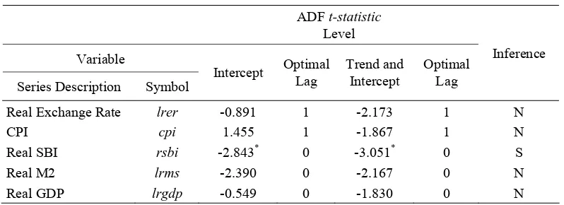
DATA AND ANALYSIS ADF Test Result
at significance level 1%, 5% and 10% succes-sively -3.52, -2.90 and -2.59. The only significant variable is SBI, meaning that null unit root hypothesis cannot be rejected for four variables, that is Real Exchange Rate, CPI, M2 and Real GDP at significance level 5%, unexceptionally, stationary SBI variable at significance level 10% , in which statistic value t is 10% bigger than critical value of MacKinnon, that is -2.59. One variable is considered stationary on the criteria of ADF test if the absolute value is bigger that MacKinnon’s critical value.
Based on the preceding discussion on the test result, macroeconomic variables on Indonesian economy seemingly will depend on several structural break caused by shocks due to the presence of government policy intervention and/or basic economic structural change which gives impact on the series, hence, the application of conventional Unit Root test (ADF) to such variable will likely bias towards the non-rejected existence of unit root.
Due to the weakness of conventional Unit Root Test (ADF), it bears a serious conse-quence when the data generating process contains structural break, the conventional unit root test will have a weak experiment outcome. Therefore, the failure of putting at least once structural break into consideration at the trend function, will bear the fact that the result of unit root test usually biases towards the non-rejected of null unit root hypothesis (Perron, 1989; 1997).
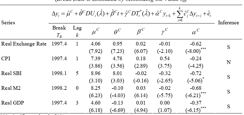
ZA Test Result
The following table 4 shows the test result of structural break using ZA procedure (1992). The estimated result at table 4 can be elaborated into several important aspects. The first, co-efficiency of the estimated result of break dummy and is, in whole, statisti-cally significant, different from zero (using a conventional critical value), which means it is in favor of the perspective that at least, there is a structural change in the intercept that occurs as long as the sample period for all variables investigated. Therefore, there is a Table 3. Conventional Unit Root test (ADF-test)
ADF t-statistic
Level
Variable
Series Description Symbol
Intercept Optimal Lag
Trend and Intercept
Optimal Lag
Inference
Real Exchange Rate lrer -0.891 1 -2.173 1 N
CPI cpi 1.455 1 -1.867 1 N
Real SBI rsbi -2.843* 0 -3.051* 0 S Real M2 lrms -2.390 0 -2.167 0 N Real GDP lrgdp -0.549 0 -1.830 0 N
*** shows the rejection of null hypothesis at significance level 1% ** shows the rejection of null hypothesis at significance level 5%, and * shows the rejection of null hypothesis at significance level 10%
Hypothetical experiment of ADF is based on the critical value of MacKinnon’s (1990). The lag length is based on Schwarz Info Criterion (1978).
S shows stationary and N shows non-stationary
substantial proof that perhaps those variables are reliant on a single permanent shock due to the structural change or the fundamental change of economic policy. Secondly, 4 out of 5 trend variables are significant; it indicates that series undergo fluctuating trend. Third, co-efficiency of estimated result for is statis-tically significant for 4 out of 5 variables (the only Real GDP (lrgdp), it indicates that at least there is one significant structural change at trend that occurs on minimally 4 variables investigated.
The identification of breakpoint TB with ZA procedure (1992) for all variables investi-gated has something worth observing, namely, the same breakpoint, (Q4 1997) for Exchange Rate variable (rer), Consumer’s Price Index (CPI), and Real GDP (lrgdp). When observed historically, we can draw an important conclu-sion that the same breakpoint resulted from
the simultaneity of financial crisis that ob-structed Indonesia in the late 1997.
Real Exchange Rate variable (lrer), historically, ever went through quite big and persistent depreciation. In the first quarter of 1998/89, Indonesian Rupiah’s exchange rate went through a quite sharp depreciation to the lowest level, namely, in June 1998 (Bank Indonesia, 1999). It was triggered by the weakness of Indonesian fundamental econ-omy which is reflected by the high level of inflation and the sharpness of economic contraction. Monetary expansion that occurred during this period stimulated the rising demand in the foreign currency market, which in turn, weakened rupiah’s exchange rate. The efforts of prevailing over foreign debt for the private sector which had not come up with clear-cut solution and the congealment of Indonesian banking credit line by foreign Table 4. The Result of Unit Root Test with Once Breakpoint Identified Endogenously in the
Intercept and Slope at the Trend Function (Model C)
(Break Date is Estimated by Minimizing the Value t)
*
1 1
ˆ ˆ ˆ ˆ ˆ ˆ
ˆ ( ) ( ) ˆ ˆ
k
C C C C C C
t t t t j t j t
j
y DU t DT y c y e
Series
Break
TB
Lag
k
C
C C C C
Inference
Real Exchange Rate 1997.4 1 4.06 0.95 0.02 -0.01 -0.62 (7.92) (7.23) (6.07) (-2.10) (-8.00)*** S CPI 1997.4 1 7.39 4.78 0.18 0.54 -0.24
(3.86) (3.56) (2.89) (3.75) (-4.25) N Real SBI 1998.1 5 8.96 8.01 -0.02 -0.32 -0.72
(3.10) (3.03) (-0.16) (-2.65) (-5.06)* S Real M2 1998.2 0 8.25 -0.10 0.03 -0.02 -0.68
(6.23) (-4.03) (6.14) (-5.75) (-6.21)*** S Real GDP 1997.4 3 4.60 -0.13 0.01 0.00 -0.37
(6.18) (-6.69) (4.94) (1.07) (-6.15)*** S *** significance level of 1%
** significance level of 5% * significance level of 10%
S indicates stationary and N indicates non-stationary
parties contributed to the pressure of Indone-sian Rupiah’s exchange rate.
Another indisputable important factor is the instability of Indonesian socio-political condition, following the unrests/riots in May 1998, which diminished the credibility of national economy. The low credibility and the swelling speculative activity –reflected on the sharply-increasing swap premium– has brought about stronger pressure on Indonesian rupiahs. Other than that, the weakening exchange rate of yen that attained 146.0 per dollar in June 1998 also has implication on the fall of the exchange rate of Asian countries’ currency, unexceptionally Indonesian cur-rency (Bank Indonesia, 2000).
Consumers’ Price Index (CPI) variable also identifies breakpoint (Q4 1997), in which the inflation rate reached 77.6 percent. The rising pressure of the main price derives from the supply side as a consequence of the sharp depreciation in that year and the decreasing supply of goods. The weakening exchange rate of rupiah results in the costly imported goods, which in turn, incites the price hike in general. Meanwhile, the goods supply de-creases sharply due to the decreasing produc-tion activity, the low producproduc-tion of crops, and the poor disturbed line of distribution which resulted from the damage of trade centers following the social chaos/riots in May 1998. Moreover, large monetary expansions also give pressure on the inflation in the above-mentioned period (Bank Indonesia, 1999).
The last variable which identifies break-point (Q4 1997) is real GDP variable (lrgdp), in which the economic growth experienced contraction as much as 13.7 percent in 1998 when compared with the one in 1997 which still had an expansion of 4.9 percent. Such a deep contraction span caused a drastically decreasing social prosperity, the widespread of unemployment, thus increased the intensity of social sentiments.
On the demand side, the sharp economic contraction resulted from the fall of domestic demand, mainly of household consumptions and private investments. The decreasing con-sumption of household is contributable to the weakening real income and the wealth value (wealth effect) as the result of prolonged crisis. At the same time, the large decrease of private investments is due to some constraint faced by private sector to curb with the unbalanced sheet, as a consequence of the occurrence of miss match either in term of time period or the currency. On the supply side, the economic contraction takes place in almost the whole private sector except for agricultural sector, especially of which pro-duces export commodity. The business sector that goes through the deepest contraction is the construction and finance sector, as a direct impact of the weakening exchange rate of Rupiah (Bank Indonesia).
hypo-thesis unit root, can’t be rejected for Consum-ers’ Price Index variable. Next, all the estimated coefficiences, at dummy variables because of the changes in the intercept and the
(C
and C
) is significant at significance level 5 percent except for the dummy variable of Real GDP shifts in the slope.
Figure 2. Estimation Plot in Determining Time of the Structural Break with ZA Procedure that Allows Breakpoint in the Intercept and the Slope of the Trend Function (Model C)
-10.0
Zivot-Andrews Unit Root Test for Real Exchange Rate
t-ra
Zivot-Andrews Unit Root Test for CPI
t-ra
Zivot-Andrews Unit Root Test for Real SBI
t-ra
1993 1994 1995 1996 1997 1998 1999 2000 2001 2002 2003 2004 2005
Zivot-Andrews Unit Root Test for Real Money Supply (M2)
t-ra
Zivot-Andrews Unit Root Test for Real GDP
The strategy of unit root test with ZA methodology bears various outcomes, one of whose structural break is mostly significant and stationary in treating almost all data of the variables investigated. This empirical finding is consistent with the original finding of ZA (1992) suggesting that some series which are originally found non-stationary when a con-ventional unit root test (ADF) is used now turns out stationary after considering the en-dogenous structural break of the ZA-test (1992).
CONCLUSIONS
This paper has identified and explained the appropriate determination of time for the main structural break on macroeconomic ma-jor variables for Indonesian economy, using quarterly data time series period of Q1 1990-Q4 2008. The strategy to reach the objective of this paper is by detecting structural break adopting Divot and Andrews approach (1992). The investigation is determined endogenously at most of single structural break in each series.
The empirical finding reported at table 3 with conventional unit root test (ADF) gives enough proof to the null hypothesis of unit root towards almost all variables investigated (null unit root hypothesis cannot be rejected to every series investigated at conventional significance level 5%). Different result is shown at table 4 after considering the signifi-cance of most structural break in data series that gives effect in the intercept and trend, a result of ZA test. Such a result indicates that there are at least four unit root are rejected out of five variables investigated at significance level 1% and 10%.
As a whole, endogenous determination of the presence of structural change on data series, correlated with that of Asian crisis that expanded so widely all the way to Indonesia in 1997-1998. Such crisis had brought about economic contraction, namely on some vari-ables investigated in the observed period.
This research finding has given new horizon related to matter of structural break on data and has given enough comprehensive, useful proof for further exploration, especially those that use time series data on Indonesian macro economy. The ZA-test which is used in this observation is merely to detect a single structural break (not multiple breaks). Because series show the potential structural break which occurs more than once, to obtain a more accurate result, it is necessary that the following research apply the unit root test method with the consideration of two or more structural breaks which are endogenously determined2.
REFERENCES
Anonim, 2009. EViews 7 User’s Guide I & II,
Quantitative Micro Software. CA: Irvine. Bai, J., and P. Perron, 2003. “Computation
and Analysis of Multiple Structural Changes Models”. Journal of Applied Econometrics, 18, 1 – 22.
Baltagi, B. H., 2011. Econometrics. 5th ed. Berlin, Heidelberg: Springer-Verlag. Banerjee, A., Lumsdaine, L. Robin, and J.H.
Stock, 1992. “Recursive and Sequential Tests of the Unit Root and Trend Break Hypothesis: Theory and International Evidence”. Journal of Business and Economic Statistics, 10 (3), 271–287. Bank Indonesia. “Laporan Tahunan
Pereko-nomian Indonesia” [Annual Report of Indonesian Economy]. Jakarta: Bank Indonesia.
Christiano, L. J., 1992. “Searching for a Break in GNP”. Journal of Business And Economic Statistics, 3, 237-250.
Enders, W., 2004. Applied Econometric Time Series. 2nd ed. New York: John Wiley & Sons, Inc.
Glynn, J., P. Nelson, and V. Reetu, 2007. “Unit Root Tests and Structural Breaks: a
2
Survey With Application”. Revista De Metodos Cuantitativos Para La Economia Y La Empresa, 3, 63-79.
Gujarati, D.N. and D.C. Porter, 2009. Basic Econometrics. 5th ed. New York: McGraw-Hill.
Harris, R., 1995. Using Cointegration Analy-sis in Econometric Modelling. England: Prentice-Hall.
Harris, R. and R. Sollis, 2003. Applied Time Series Modelling and Forecasting. England: John Wiley and Sons.
Johnston, J. and J. Dinardo, 1997. Economet-ric Methods. 4th ed. New York: McGraw-Hill International.
Jomo, K. S., 1997. Southeast Asia’s Misunderstood Miracle: Industrial Policy and Economic Development in Thailand, Malaysia and Indonesia. In Sharma, S., 2003. The Asian Financial Crisis: Crisis,
Reform, and Recovery. New York:
Manchester University Press.
Krugman, P.R. and M. Obstfeld, 2007. Inter-national Economics: Theory and Policy, 7th edition. New York: Addison-Wesley. Lumsdaine, R.L., and D.H. Papell, 1997.
“Multiple Trend Breaks and the Unit Root Hypothesis”. Review of Economics and Statistics, 79(2), 212-18.
Leybourne, S.J and P. Newbold, 2003. “Spurious Rejections by Cointegration Tests Induced by Structural Breaks”.
Applied Economics, 35(9), 1117-1121. Maddala, G.S. and I. Kim, 1998. Unit Roots
Cointegration and Structural Change.
New York: Cambridge University Press.
Marashdeh, H. and E.J. Wilson, 2005. “Struc-tural Changes in the Middle East Stock Markets: the Case of Israel and Arab Countries”. University of Wollongong Economics Working Paper Series, 05 (02), 1-15.
OECD, 2008. OECD Economic Surveys: Indonesia Economic Assessment. Jakarta: OECD.
Pahlavani, M, A. Valadkhani, and A. Worthington, 2005. “Testing for Struc-tural Breaks in Australia’s Monetary Aggregates and Interest Rates: an Application of Innovational Outlier and Additive Outlier Models”. University of Wollongong Economics Working Paper Series, 05 (02), 1-15.
Perron, P., 1989. “The Great Crash, the Oil Price Shock, and the Unit Root Hypo-thesis”. Econometrica, 57(6), 1361-1401. Perron, P. and T. J. Vogelsang, 1992.
“Nonstationarity and Level Shifts with an Application to Purchasing Power Parity”.
Journal of Business and Economic Statistics, 10, 301-320.
Perron, P., 1997. “Further Evidence on Break-ing Trend Functions in Macroeconomic Variables”. Journal of Econometrics, 80 (2), 355-385.
Pincus, J. and Ramli, R., 2001. Indonesia: From Showcase to Basket Case. In Chang, et al. (eds). Financial Liberaliza-tion and the Asian Crisis. New York: Palgrave Macmillan.
Radelet, S., 1999. “Indonesia’s Long Road to Recovery”, unpublished paper, March. Harvard Institute for International Devel-opment. In Sharma, S., 2003. The Asian Financial Crisis: Crisis, Reform, and
Recovery. New York: Manchester
University Press.
Sharma, S., 2003. The Asian Financial Crisis: Crisis, Reform, and Recovery. New York: Manchester University Press
Siswanto, J., 2007. “Pengalaman IMF dalam Menangani Krisis di Beberapa Negara
[IMF’s Experience in Handling Crisis of Some Countries]”. In Arifin, S., et al.
Stock, J.H. and M.W Watson, 2007.
Introduction to Econometrics. 2nd ed, Boston: Pearson/Addison-Wesley.
Tjahjono, E.D., and D.F Anugrah, 2006. “Faktor-faktor Determinan Pertumbuhan Ekonomi Indonesia [Determining Factors
of Indonesian Economy Development]”, WP/08, Bank Indonesia.