FEASIBILITY OF MACHINE LEARNING METHODS FOR SEPARATING WOOD AND
LEAF POINTS FROM TERRESTRIAL LASER SCANNING DATA
D. Wanga,∗, M. Hollausa, N. Pfeifera
a
Department of Geodesy and Geoinformation, TU Wien, Vienna 1040, Austria (di.wang, markus.hollaus, norbert.pfeifer)@geo.tuwien.ac.at
KEY WORDS:Terrestrial Laser Scanning, Wood-leaf classification, Machine Learning, Feature selection
ABSTRACT:
Classification of wood and leaf components of trees is an essential prerequisite for deriving vital tree attributes, such as wood mass, leaf area index (LAI) and woody-to-total area. Laser scanning emerges to be a promising solution for such a request. Intensity based approaches are widely proposed, as different components of a tree can feature discriminatory optical properties at the operating wavelengths of a sensor system. For geometry based methods, machine learning algorithms are often used to separate wood and leaf points, by providing proper training samples. However, it remains unclear how the chosen machine learning classifier and features used would influence classification results. To this purpose, we compare four popular machine learning classifiers, namely Support Vector Machine (SVM), Na¨ıve Bayes (NB), Random Forest (RF), and Gaussian Mixture Model (GMM), for separating wood and leaf points from terrestrial laser scanning (TLS) data. Two trees, anErytrophleum fordiiand aBetula pendula(silver birch) are used to test the impacts from classifier, feature set, and training samples. Our results showed that RF is the best model in terms of accuracy, and local density related features are important. Experimental results confirmed the feasibility of machine learning algorithms for the reliable classification of wood and leaf points. It is also noted that our studies are based on isolated trees. Further tests should be performed on more tree species and data from more complex environments.
1. INTRODUCTION
Quantifying forest structure is of broad importance. For example, understanding forest foliage profile can be of particular interest for biodiversity conservation and climate adaptation, as it affects the photosynthesis and evapotranspiration processes (Ma et al., 2016). Monitoring carbon stocks in forested ecosystems requires accurate quantification of the spatial distribution of wood volume (Levick et al., 2016). Moreover, description of 3D structure helps to investigate species competition, wood production, and ecosys-tem and agro-ecosysecosys-tem dynamics (B´eland et al., 2014). For mapping forest structure, laser scanning is widely used in past decades. Laser scanning technique, also known as light detec-tion and ranging (lidar), acquires 3D coordinates of objects over a large scale. In addition, full-waveform laser scanners are able to measure the scattering properties of vegetation in a quantitative way (Wagner et al., 2008). Therefore, laser scanning generates a high potential for forest related studies.
Assessment of canopy structure at tree or branch scale can be difficult with laser scanning data acquired from satellite and air-borne platforms (Tao et al., 2015). Terrestrial Laser Scanning (TLS), on the other hand, has been established as an efficient tool for acquiring 3D data used for a range of fine-scale forest studies (Liang et al., 2016), including stem mapping (Liang et al., 2012), tree height measurement (Olofsson et al., 2014), diameter estima-tion (Wang et al., 2017), stem curve retrieval (Wang et al., 2016), biomass calculation (Kankare et al., 2013), and leaf area index (LAI) estimation (Zheng et al., 2013). To better retrieve forest ecological attributes, it is often necessary to separate wood and leaf components of trees (Tao et al., 2015). For example, esti-mation of LAI requires to screen out wood points, otherwise the wood returns will artificially increase the apparent foliage content (B´eland et al., 2014).
Wood-leaf point separation for TLS data is challenging. In gen-eral, existing methods can be categorized into two groups;
inten-∗Corresponding author
sity based and geometry based. Intensity based methods (Pfen-nigbauer and Ullrich, 2010; B´eland et al., 2014) use radiomet-ric information of objects captured by a laser scanner. The as-sumption is that wood and leaf components have different op-tical properties at the operating wavelength of the laser scanner (Tao et al., 2015). By determining a proper intensity threshold, wood and leaf points can be separated. However, intensity cap-tured by a laser scanner needs an instrument specific radiometri-cal radiometri-calibration before including it in further processing (Calders et al., 2017). Recently developed multi-wavelength (e.g., hyper-spectal) scanners can help to better solve such a task (Li et al., 2013; Hakala et al., 2012; Vauhkonen et al., 2013). However, these scanners are still in an early development stage, and not yet widely available. Geometry based methods only use 3D coor-dinates of objects captured by a laser scanner. Local structure-related saliency information are derived from 3D points and su-pervised machine learning methods such as Support Vector Ma-chine (SVM) (Yun et al., 2016) and Gaussian Mixture Model (GMM) (Ma et al., 2016) are often employed to classify wood and leaf points. Some direct geometric methods were also re-ported (Tao et al., 2015). Nevertheless, geometry based machine learning methods are rarely systematically examined for wood-leaf classification, although it is a well-known and widely adapted technique for other classification tasks (Weinmann et al., 2013, 2017; Brodu and Lague, 2012). There is a vast need to exploit 3D geometry based approaches for separating wood and leaf points, as 3D coordinates are the most fundamental information acquired by any laser scanners. For machine learning methods, various classifiers were used in previous studies (Yun et al., 2016; Ma et al., 2016). The lack of comparable studies calls for a specific examination on how the chosen machine learning classifier and features used would influence classification results.
ma-chine learning models used for separating wood and leaf points are presented. Finally, in section 4 the results are presented and discussed in section 5. Conclusion is given in section 6.
2. MATERIALS
2.1 Erytrophleum fordii
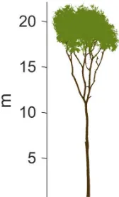
TLS data of an evergreen sub tropical tree,Erytrophleum fordii, were provided by Hackenberg et al. (2015). The data were ac-quired in October 2013 from eight scan positions. The acac-quired point cloud was further manually cleaned, as the tree crown in-teracts with other trees. Therefore, points from adjacent trees’ foliage need to be removed. The cleaned point cloud for the Ery-trophleum fordiitree contains∼3.9 million points. The average distance between two adjacent points is∼5 mm (Figure 1).
Figure 1. Point cloud of theErytrophleum fordii.
2.2 Betula pendula
Hyperspectral TLS data of another silver birch tree (Betula pen-dula, Figure 2) were provided by Puttonen et al. (2016). The single-scan data feature radiometrical information of the scanned tree, in addition to the 3D XYZ coordinates. The average dis-tance between two adjacent points is∼1 cm. Measurements were carried out using a Hyperspectral Laser Scanner (HSL) from the Finnish Geospatial Research Institute (FGI) (Hakala et al., 2012). Laser radiometry was calibrated by setting up an external refer-ence plate. For more information about the HSL data, readers are referred to Puttonen et al. (2016).
3. METHODS
3.1 Feature Calculation
Twenty-six 2D and 3D geometry-based point cloud features ex-tracted for each data set were described in Table 1. The features were originally proposed and used in Weinmann et al. (2015) for urban area scene analysis. Local 3D features are inferred from the distribution of neighboring points of every point. Structure saliency such as planar, linear, and scattering can be inferred from the eigenvalues of the decomposed covariance matrix (Equation 1).
Covp=
PK
i=1(pi−p)(pi−p)
T
K , (1)
wherepi={xi, yi, zi}T
is a 3D point andpis the barycenter of theKnearest neighboring points. 2D feature calculation involves
Figure 2. Point cloud of theBetula pendula, silver birch.
a projection of points onto the horizontal plane. For details of fea-ture extraction procedures, the readers are referred to Weinmann et al. (2015).
3.2 Feature Selection
The high dimensionality of the input data may exhibit redundancy and can be potentially reduced by various feature selection algo-rithms. Moreover, feature selection may attenuate the over-fitting problem in multivariate classification methods (Geiß et al., 2015). Feature selection methods can be grouped into three categories; wrappers, embedded, and filters (Guyon et al., 2008). Wrappers methods evaluate a subset of features by accuracy estimates and require trained classifiers. Embedded methods embed the selec-tion process into the classifier learning. On the other hand, filter methods explore the intrinsic properties of the data , and thus op-erate independently with respect to classifiers. In this study, we employ the filter method for feature selection for its simplicity and efficiency, although more robust and concrete methods are used in previous studies (Weinmann et al., 2013).
A fast and effective filter method is the Fishermethod (Gu et al., 2012). This method computes a score (Fisher score) accord-ing to a ratio of interclass separation and intraclass variance for each feature and ranks them. The scores reflect the discriminative power of each feature. In this study, we apply theFishermethod for bothErytrophleum fordiiand silver birch datasets. The resul-tant rankings are given in Table 1. Consequently, the classifier learning was performed for 5, 10, 15, 20, and 26 features accord-ingly, based on the rankings.
3.3 Machine Learning Classifiers
Wood-leaf separation is a binary classification problem. Givenm training samples,(yi,xi)i= 1, . . . mwith labelsyi∈ {1,−1}
andndimensional feature vectors,xi ∈Rn, the objective is to
find a functionf( ;α) : x 7→ ythat represents the classifier
y=f(x;α), whereαare all the parameters of the classifier.
In this study, we examine the feasibility of four machine learn-ing algorithms, SVM, NB, RF, GMM, for wood-leaf separation. In this section, the fundamentals and principles of the four used machine learning algorithms are briefly summarized.
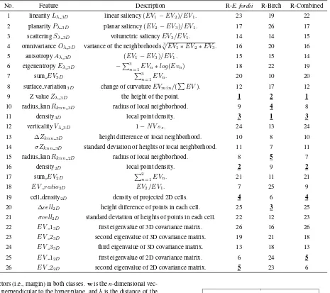
Table 1. Features extracted from the point cloud.EVdenotes the eigenvalue andN Vis the normal vector.EV sare sorted in a descend manner. ”R-” is the abbreviation of ”Ranking” form feature selection. ”R-Combined” means that the feature set is a combination of data from both trees. Top 5 ranked features are underlined.
No. Feature Description R-E. fordii R-Birch R-Combined
1 linearityLλ3D linear saliency(EV1−EV2)/EV1. 23 19 22
2 planarityPλ3D planar saliency(EV2−EV3)/EV1. 17 26 17
3 scatteringSλ3D volumetric saliencyEV3/EV1. 14 14 15
4 omnivarianceOλ3D variance of the neighborhoods
3
√
EV1∗EV2∗EV3. 16 20 16
5 anisotropyAλ3D (EV1−EV3)/EV1. 15 15 14
6 eigenentropyEλ3D −P3n=1EVn∗log(Evn) 18 22 19
7 sumEV3D P
3
n=1EVn. 20 10 20
8 surface variation3D change of curvatureEVmin/(PEV). 12 17 12
9 Z valueZλ3D the height of the point. 1 2 1
10 radius knnRknn3D radius of local neighborhood. 9 4 8
11 density3D local point density. 3 1 3
12 verticalityVλ3D 1−N V sz. 24 13 24
13 ∆Zknn3D height difference of local neighborhood. 10 8 10
14 σZknn3D standard deviation of heights of local neighborhood. 11 7 11
15 radius knnRknn2D radius of local neighborhood. 8 5 7
16 density2D local point density. 2 9 2
17 sumEV2D P2n=1EVn. 21 11 21
18 EV ratio2D EV2/EV1. 7 25 9
19 cell density2D density of projected 2D cells. 4 6 4
20 ∆cell2D height difference of points in each cell. 25 3 25
21 σcell2D standard deviation of heights of points in each cell. 22 12 23
22 EV 13D first eigenvalue of 3D covariance matrix. 26 16 26
23 EV 23D second eigenvalue of 3D covariance matrix. 19 21 18
24 EV 33D third eigenvalue of 3D covariance matrix. 13 18 13
25 EV 12D first eigenvalue of 2D covariance matrix. 6 24 5
26 EV 22D second eigenvalue of 2D covariance matrix. 5 23 6
vectors (i.e., margin) in both classes.wis then-dimensional
vec-tor perpendicular to the hyper-plane, andbis the distance of the closest point on the hyper-plane to the origin. The classifier is then
f(x) =sgn
m X
i=1
λiyiK(xi,xj) +b
!
, (2)
whereλis the weight andK(xi,xj)is akernel functionK(xi,xj) = Φ(xi)·Φ(xj), subjects toyi(<w,xi>+b)−1≥0.
3.3.2 Na¨ıve Bayes NB is a statistical approach based on Bayes’s theorem (Marcot et al., 2006). It assumes that the features are conditionally independent given the class,
p(x|y) = m Y
i=1
p(xi|y). (3)
Therefore, from the Bayes’s theorem, the posterior probability of a feature vector to be part of a certain class is
p(y|x) = p(y)
Qm
i=1p(xi|y)
p(x) , (4)
wherep(y)is the prior probability of the class. A point will be labeled as the class with the highest probability.
Figure 3. Evaluation of number of classification trees to be grown.
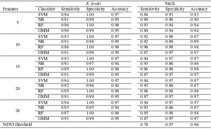
determina-Table 2. Statistical evaluation of machine learning classifiers for wood-leaf separation.
E. fordii birch
Features Classifier Sensitivity Specificity Accuracy Sensitivity Specificity Accuracy
5
SVM 0.94 1.00 0.97 0.88 0.93 0.93
NB 0.91 0.99 0.95 0.90 0.90 0.90
RF 0.96 1.00 0.98 0.93 0.94 0.94
GMM 0.90 0.99 0.95 0.88 0.94 0.94
10
SVM 0.93 1.00 0.97 0.92 0.98 0.97
NB 0.91 0.98 0.95 0.92 0.89 0.89
RF 0.96 1.00 0.98 0.96 0.98 0.98
GMM 0.91 0.99 0.95 0.87 0.97 0.97
15
SVM 0.93 1.00 0.97 0.94 0.97 0.97
NB 0.91 0.97 0.94 0.93 0.86 0.86
RF 0.95 1.00 0.98 0.96 0.98 0.98
GMM 0.91 0.99 0.95 0.87 0.97 0.97
20
SVM 0.94 1.00 0.97 0.94 0.97 0.97
NB 0.92 0.96 0.94 0.93 0.86 0.87
RF 0.95 1.00 0.98 0.96 0.98 0.98
GMM 0.91 0.99 0.95 0.87 0.97 0.97
26
SVM 0.94 1.00 0.97 0.94 0.97 0.97
NB 0.93 0.95 0.94 0.93 0.86 0.87
RF 0.97 1.00 0.98 0.95 0.98 0.98
GMM 0.91 0.99 0.95 0.87 0.97 0.97
NDVI threshold 0.78 0.97 0.96
tion is based on a majority votes fashion. RF has proven to be an accurate and robust classification and regression approach, even on noisy data (Geiß et al., 2015).
When employing RF, two necessary parameters need to be spec-ified; the number of classification treentreesand the number of input featuresmf tused at each node (Geiß et al., 2015). A higher number of ntrees increases model accuracy until convergence. We used our data with all features to train models. We observe that in our study, the model performance converges at the point of approximate 60 trees (Figure 3). However, since our data set is not large enough for us to consider a trade off for computa-tion time, we keep the number as 100. We set another parameter, mf t=√p, where p denotes the number of input feature, as sug-gested by Breiman (2001).
3.3.4 Gaussian Mixture Model GMM is a modeling tech-nique that uses a probability distribution to estimate the likeli-hood of a given feature vector. The assumption is that classes obey a normally distributed density function. For a binary classi-fication problem, the continuous probability density function can be approximated as a linear combination of two probability den-sity functions (Ma et al., 2016),
p(x) = m X
k=1
wkp(x|k) (5)
where wk is the weight for each probability density function. p(x|k)is the conditional probability of a pointxbelonging to the kth density function.The probability that a pointxilies within the a distribution with parametersµandΣis given by
N(µk,Σk) =
In this study, manually delineated training points are used to train the GMM model. TheExpectation-Maximization algorithm (EM)
is used to estimate theµandΣof each class. Consequently, a point will be labeled as the class with the highest probability.
3.4 Evaluation
The performance of each classifier is evaluated based on three statistical indexes; sensitivity, specificity, and accuracy. Sensitiv-ity measures the correctly classified positive samples (true posi-tive rate,T P). In this study, it represents that the correct rate for wood points. Specificity gives the true negative rate (T N), thus it measures the correct rate for leaf points. Accuracy (ACC) gives the overall correctness by
ACC= T P+T N
P+N , (7)
wherePandNare the number of real positive (wood) and neg-ative (leaf) samples.
4. EXPERIMENTS AND RESULTS
We manually selected approximate 10% points from each tree as the training data for the machine learning classifiers. These train-ing points are evenly distributed from the bottom to the top of each tree. Consequently, four machine learning classifiers were trained accordingly with different feature sets. The statistical per-formance indices are summarized in Table 2.
fordiitree, although in this case the trend was weak. The reason may be that the assumption in NB that a particular feature is inde-pendent of the value of any other feature was violated when more features were involved. In such a case, the Bayesian Network model (Friedman et al., 1997) will be more suitable. In addition, NB is known to have difficulties when dealing with unbalanced data.
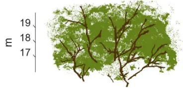
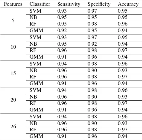
We observed that the high classification accuracy of the Ery-trophleum fordiimight be caused by the fact that the distributions of its stem and crown are essentially very well distinct. To assess the performances of machine learning classifiers in regions where leaf and wood components are heavily interacted, we selected a subset point cloud between 16 and 20 m above ground of the
Erytrophleum fordii(Figure 6), and ran the experiments on this subset. The results are given in Table 3. The accuracy remained almost identical compared to those from the whole point cloud, indicating that machine learning algorithms can commendably separate leaf and wood components by providing proper training samples.
For the silver birch, calibrated spectral attributes exist. Therefore, leaf and wood can be separated from the spectral information of each point as well. This is based on the fact that different com-ponents of a tree feature discriminatory optical properties at the operating wavelengths of the laser scanning system (Tao et al., 2015). In this study, the birch leaf and wood were separated with a hard normalized difference vegetation index (NDVI) threshold value of 0.2. All points that have NDVI value less than 0.2 were labeled as wood components, and vice versa. The accuracy of the spectral method is included in Table 2. The sensitivity (i.e., accuracy for wood identification) is lower than those from ma-chine learning algorithms, mainly because some higher parts of the stem were misclassified as leaves.
Figure 4. Performance of four classifiers for theErytrophleum fordiias a function of the different feature sets. Feature sets were determined based on theFisherfilter method described in section 3.2.
5. DISCUSSION
5.1 Classifier Performance
As summarized in the Tables 2 and 3, the performances of se-lected machine learning classifiers are comparable to and surpass-ing published studies (Ma et al., 2016; Tao et al., 2015). In our tests, RF model produced best results, proving that RF might be very well suitable for wood-leaf classification. This can also be
Figure 5. Performance of four classifiers for the silver birch as a function of the different feature sets. Feature sets were deter-mined based on theFisherfilter method described in section 3.2.
Figure 6. A crown subset (i.e., 16 - 20 m) of theErytrophleum fordii. Branches and leaves heavily interact.
Figure 7. Classification results of RF model forErytrophleum fordii. Left part shows the wood components and right part shows the leaf points.
Table 3. Statistical evaluation of machine learning classifiers for the crown subset of theErytrophleum fordiiwith 5, 10, 15, 20, and 26 features.
Features Classifier Sensitivity Specificity Accuracy
5
Figure 8. Classification results of RF model for silver birch. Left part shows the wood components and right part shows the leaf points.
others’. NB model performed worse in this study and might not be suitable for leaf-wood separation, unlike its high efficiency in text classification (Kim et al., 2006). GMM model is typi-cally used in unsupervised classification problems (Koo et al., 2014), although it was previously used in separating leaf, wood, and ground points (Ma et al., 2016). We briefly tested the per-formance of the GMM classifier without training data, so that the data were clustered into two groups in the feature space. We ob-tained an accuracy of 93% and 91% for theErytrophleum fordii
and silver birch, respectively, which are lower than that of the supervised GMM.
5.2 Feature Importance
In this study, features were ranked based theFisherfilter feature selection method (Table 1). Furthermore, feature sets with differ-ent sizes based on the rankings are tested. For both trees, point height and local density seem to be the most vital features, as
they were both ranked as top 5. This indicates that local density characteristics might play a vital role in leaf-wood separation. However, both of them are bound to perform worse in a more complex scene. Commonly used structure inferring features such as linearity and planarity turned out to be less important as they were ranked as non-significant (e.g., 50% in the case of the lat-ter). This can also be justified from the performances of various feature sets. For both trees, the first 10 best features according to the ranking are enough to stabilize the model accuracy, meaning that features such as linearity and planarity are not necessary to be included in such a wood-leaf classification issue. However, we note that feature selection should consider the local tree structure characteristics, such as tree species. In addition, more feature se-lection approaches should be tested, possibly in connected with the chosen machine learning model. Such methods are known as
wrappers.
5.3 Training Sample Delineation
In this study, training samples were manually and evenly selected from the bottom to the top of each tree. The selected training data take up around 10% of the whole point cloud. In order to as-sess the influences of training samples, we re-selected a different training sample set with 1m height intervals for the crown subset of the Erytrophleum fordii(Figure 6). The re-selected training sample only occupies ∼1% of the whole data. The classifica-tion results are compared in Table 4. It is noted that the accuracy decreased when less and unevenly distributed training data were used. In particular, model sensitivities reduced drastically, mean-ing that some wood points were misclassified as leaf points. This implies that the local geometry properties of branch points are not well represented by a small set and vertically spaced training data.
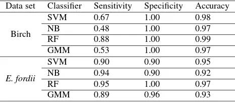
In addition, we trained all classifiers with training data from both trees, meaning that half training data are from theErytrophleum fordiiand left are from the silver birch. The results for the Ery-trophleum fordii remain identical compared to those classifiers trained with onlyErytrophleum fordiidata (Table 5 and Table 2). However, the results for the silver birch are worse, especially in terms of the sensitives, except the RF model. This indicates that the wood parts of the silver birch are severely misclassified as leaf points when using the classifiers trained with a combined train-ing set. RF is immune from this situation, again indicattrain-ing its efficiency and capability for such as task.
Table 4. Comparison of performances with different training data on the crown subset. Samplef denotes the manually selected 10% training set. Samplesrefers to a training set with 1m height intervals.
Classifier Sample Sensitivity Specificity Accuracy
SVM f 0.94 0.98 0.96
Table 5. Performances of all classifiers trained with a combined training set from both trees.
Data set Classifier Sensitivity Specificity Accuracy
Birch
from TLS data. In general, there is a lack of comparative stud-ies of machine learning algorithms for such problems. Our study highlighted the feasibility of the methodology. Specifically, two trees were tested, anErytrophleum fordiiand a silver birch. Twenty-six geometry-based features were extracted and individually ranked by a filter feature selection method. Various feature sets and train-ing data were tested. Our results show that machine learntrain-ing al-gorithms can efficiently separate wood and leaf point from TLS data with an accuracy of, in general, more than 95%. Evenly dis-tributed training data are recommended, as sparse training data can reduce the classification accuracy especially for branches in-side the tree crown. It is noted that our studies were performed on purer data sets. More tests on tree data from more complex natural conditions should be carried out in the future. In addition, more tree species should be tested.
ACKNOWLEDGEMENTS
The study was supported by the project ”The influence of Biomass and its change on landSLIDE activity” (BioSLIDE) within the research program Earth System Sciences (ESS) of the Austrian Academy of Science ( ¨Osterreichische Akademie der Wissenschaften,
¨
OAW) and financed by the Federal Ministry of Science and Re-search (BMWF). The authors also thank the Austrian ReRe-search Promotion Agency (FFG) for providing financial support via the project no. 860021. Special thanks are due to three referees for their constructive reviews that improved the manuscript signifi-cantly.
REFERENCES
B´eland, M., Baldocchi, D. D., Widlowski, J.-L., Fournier, R. A. and Verstraete, M. M., 2014. On seeing the wood from the leaves and the role of voxel size in determining leaf area distribution of forests with terrestrial lidar. Agricultural and Forest Meteorology 184, pp. 82–97.
Breiman, L., 2001. Random forests. Machine learning 45(1), pp. 5–32.
Brodu, N. and Lague, D., 2012. 3d terrestrial lidar data classifi-cation of complex natural scenes using a multi-scale dimension-ality criterion: Applications in geomorphology. ISPRS Journal of Photogrammetry and Remote Sensing 68, pp. 121–134.
Calders, K., Disney, M. I., Armston, J., Burt, A., Brede, B., Origo, N., Muir, J. and Nightingale, J., 2017. Evaluation of the range accuracy and the radiometric calibration of multiple terrestrial laser scanning instruments for data interoperability. IEEE Transactions on Geoscience and Remote Sensing 55(5), pp. 2716–2724.
Friedman, N., Geiger, D. and Goldszmidt, M., 1997. Bayesian network classifiers. Machine learning 29(2-3), pp. 131–163.
Geiß, C., Pelizari, P. A., Marconcini, M., Sengara, W., Edwards, M., Lakes, T. and Taubenb¨ock, H., 2015. Estimation of seismic building structural types using multi-sensor remote sensing and machine learning techniques. ISPRS Journal of Photogrammetry and Remote Sensing 104, pp. 175–188.
Gu, Q., Li, Z. and Han, J., 2012. Generalized fisher score for feature selection. arXiv preprint arXiv:1202.3725.
Guyon, I., Gunn, S., Nikravesh, M. and Zadeh, L. A., 2008. Fea-ture extraction: foundations and applications. Vol. 207, Springer.
Hackenberg, J., Wassenberg, M., Spiecker, H. and Sun, D., 2015. Non destructive method for biomass prediction combining tls de-rived tree volume and wood density. Forests 6(4), pp. 1274–1300.
Hakala, T., Suomalainen, J., Kaasalainen, S. and Chen, Y., 2012. Full waveform hyperspectral lidar for terrestrial laser scanning. Optics express 20(7), pp. 7119–7127.
Kankare, V., Holopainen, M., Vastaranta, M., Puttonen, E., Yu, X., Hyypp¨a, J., Vaaja, M., Hyypp¨a, H. and Alho, P., 2013. Indi-vidual tree biomass estimation using terrestrial laser scanning. IS-PRS Journal of Photogrammetry and Remote Sensing 75, pp. 64– 75.
Kim, S.-B., Han, K.-S., Rim, H.-C. and Myaeng, S. H., 2006. Some effective techniques for naive bayes text classification. IEEE transactions on knowledge and data engineering 18(11), pp. 1457–1466.
Koo, S., Lee, D. and Kwon, D.-S., 2014. Unsupervised object individuation from rgb-d image sequences. In: Intelligent Robots and Systems (IROS 2014), 2014 IEEE/RSJ International Confer-ence on, IEEE, pp. 4450–4457.
Levick, S. R., Hessenm¨oller, D. and Schulze, E.-D., 2016. Scal-ing wood volume estimates from inventory plots to landscapes with airborne lidar in temperate deciduous forest. Carbon Bal-ance and Management 11(1), pp. 7.1 – 7.14.
Li, Z., Douglas, E., Strahler, A., Schaaf, C., Yang, X., Wang, Z., Yao, T., Zhao, F., Saenz, E. J., Paynter, I. et al., 2013. Separating leaves from trunks and branches with dual-wavelength terrestrial lidar scanning. In: Geoscience and Remote Sensing Symposium (IGARSS), 2013 IEEE International, IEEE, pp. 3383–3386.
Liang, X., Kankare, V., Hyypp¨a, J., Wang, Y., Kukko, A., Haggr´en, H., Yu, X., Kaartinen, H., Jaakkola, A., Guan, F. et al., 2016. Terrestrial laser scanning in forest inventories. ISPRS Jour-nal of Photogrammetry and Remote Sensing 115, pp. 63–77.
Liang, X., Litkey, P., Hyypp¨a, J., Kaartinen, H., Vastaranta, M. and Holopainen, M., 2012. Automatic stem mapping using single-scan terrestrial laser scanning. Geoscience and Remote Sensing, IEEE Transactions on 50(2), pp. 661–670.
Ma, L., Zheng, G., Eitel, J. U., Moskal, L. M., He, W. and Huang, H., 2016. Improved salient feature-based approach for automat-ically separating photosynthetic and nonphotosynthetic compo-nents within terrestrial lidar point cloud data of forest canopies. Geoscience and Remote Sensing, IEEE Transactions on 54(2), pp. 679–696.
Marcot, B. G., Steventon, J. D., Sutherland, G. D. and McCann, R. K., 2006. Guidelines for developing and updating bayesian belief networks applied to ecological modeling and conservation. Canadian Journal of Forest Research 36(12), pp. 3063–3074.
Pfennigbauer, M. and Ullrich, A., 2010. Improving quality of laser scanning data acquisition through calibrated amplitude and pulse deviation measurement. In: SPIE Defense, Secu-rity, and Sensing, International Society for Optics and Photonics, pp. 76841F–76841F.
Puttonen, E., Briese, C., Mandlburger, G., Wieser, M., Pfennig-bauer, M., Zlinszky, A. and Pfeifer, N., 2016. Quantification of overnight movement of birch (betula pendula) branches and fo-liage with short interval terrestrial laser scanning. Frontiers in plant science 7, pp. 222.1 – 222.13.
Tao, S., Guo, Q., Su, Y., Xu, S., Li, Y. and Wu, F., 2015. A geometric method for wood-leaf separation using terrestrial and simulated lidar data. Photogrammetric Engineering & Remote Sensing 81(10), pp. 767–776.
Vapnik, V., 1995. The Nature of Statistical Learning Theory. Springer.
Vauhkonen, J., Hakala, T., Suomalainen, J., Kaasalainen, S., Nevalainen, O., Vastaranta, M., Holopainen, M. and Hyypp¨a, J., 2013. Classification of spruce and pine trees using active hy-perspectral lidar. IEEE Geoscience and Remote Sensing Letters 10(5), pp. 1138–1141.
Wagner, W., Hollaus, M., Briese, C. and Ducic, V., 2008. 3d vegetation mapping using small-footprint full-waveform airborne laser scanners. International Journal of Remote Sensing 29(5), pp. 1433–1452.
Wang, D., Hollaus, M., Puttonen, E. and Pfeifer, N., 2016. Auto-matic and self-adaptive stem reconstruction in landslide-affected forests. Remote Sensing 8(12), pp. 974.1 – 974.23.
Wang, D., Kankare, V., Puttonen, E., Hollaus, M. and Pfeifer, N., 2017. Reconstructing stem cross section shapes from terrestrial laser scanning. IEEE Geoscience and Remote Sensing Letters 14(2), pp. 272–276.
Weinmann, M., Jutzi, B. and Mallet, C., 2013. Feature relevance assessment for the semantic interpretation of 3d point cloud data. ISPRS Annals of the Photogrammetry, Remote Sensing and Spa-tial Information Sciences II-5/W2, pp. 313 – 318.
Weinmann, M., Urban, S., Hinz, S., Jutzi, B. and Mallet, C., 2015. Distinctive 2d and 3d features for automated large-scale scene analysis in urban areas. Computers & Graphics 49, pp. 47– 57.
Weinmann, M., Weinmann, M., Mallet, C. and Br´edif, M., 2017. A classification-segmentation framework for the detection of in-dividual trees in dense mms point cloud data acquired in urban areas. Remote Sensing 9(3), pp. 277.1 – 277.28.
Yun, T., An, F., Li, W., Sun, Y., Cao, L. and Xue, L., 2016. A novel approach for retrieving tree leaf area from ground-based lidar. Remote Sensing 8(11), pp. 942.1 – 942.21.