Policy
ISSN: 2146-4553
available at http: www.econjournals.com
International Journal of Energy Economics and Policy, 2019, 9(2), 390-398.
Vector Autoregressive with Exogenous Variable Model and its
Application in Modeling and Forecasting Energy Data: Case
Study of PTBA and HRUM Energy
Warsono, Edwin Russel, Wamiliana, Widiarti, Mustofa Usman*
Department of Mathematics, Faculty of Science and Mathematics, Universitas Lampung, Indonesia. *Email: [email protected]
Received: 10 October 2018 Accepted: 22 January 2019 DOI: https://doi.org/10.32479/ijeep.7223
ABSTRACT
Owing to its simplicity and less restrictions, the vector autoregressive with exogenous variable (VARX) model is one of the statistical analyses frequently used in many studies involving time series data, such as finance, economics, and business. The VARX model can explain the dynamic behavior of the relationship between endogenous and exogenous variables or of that between endogenous variables only. It can also explain the impact of a variable or a set of variables on others through the impulse response function (IRF). Furthermore, VARX can be used to predict and forecast time series data. In this study, PTBA and HRUM energy as endogenous variables and exchange rate as an exogenous variable were studied. The data used herein were collected from January 2014 to October 2017. The dynamic behavior of the data was also studied through IRF and Granger causality analyses. The forecasting data for the next 1 month was also investigated. On the basis of the data provided by these different models, it was found that VARX (3,0)
is the best model to assess the relationship between the variables considered in this work.
Keywords: Vector Autoregressive Model, Vector Autoregressive with Exogenous Variable Model, Granger Causality, Impulse Response Function, Forecasting
JEL Classifications: C32, Q4, Q47
1. INTRODUCTION
Currently, the development of communication technology and the
globalization of the economy have accelerated the integration of
world financial markets. The aim of empirical economic analysis is to investigate the economics dynamic and its mechanisms. To this end, relevant economic data are needed (Gourieroux and Monfort, 1997).
Price movement in one market can easily spread to other markets.
Therefore, financial markets are more dependent on each other and
must be considered jointly to better understand the dynamics of
global finance (Tsay, 2005; 2014). The vector autoregressive (VAR) model plays an important role in modern techniques of analysis, especially in economics and finance (Hamilton, 1994; Kirchgassner and Wolters, 2007). The VAR model was introduced by Sims (1980)
as a method to analyze macroeconomic data. He developed the VAR
model as an alternative to the traditional system, which involved
several equations (Kirchgassner and Wolters, 2007). VAR is one of
the most used research tools to analyze macroeconomic time series
data in the last two decades. There are some advantages because of which the VAR model is commonly used to analyze multivariate time series: (1) The model is relatively easy to estimate, i.e., for a VAR model, LSE are asymptotically equivalent to the method of MLE and OLS; (2) the properties of the VAR model have been extensively discussed in the literature; (3) the VAR model is similar to multivariate multiple linear regression (Tsay, 2014).
Sims stressed the need to drop the adhoc dynamic restrictions in
regression models and to discard empirically implausible exogeneity assumptions (Sims, 1980). He also stressed the need to jointly
model all endogenous variables rather than one equation at a time (Kilian, 2011).
The VAR model is often used to describe the behavior of a variable over time (Al-hajj et al., 2017; Sharma et al., 2018). In this model, it is assumed that the current value can be expressed as a function of preceding values and a random error (Fuller, 1985). Hence, VAR is an easy model to analyze multivariate time series data; the VAR model is also flexible, easy to estimate, and usually gives a good fit to the data (Juselius, 2006; Fuller, 1985, Tsay, 2014, Lutkepohl, 2005). The VAR model, which involves a normal distribution, has frequently been a popular choice as a description of macroeconomic time series data (Juselius, 2006). In a VAR model of order p, VAR (p), each component of vector Xt depends linearly on its own lagged values up to p periods as
well as on the lagged values of all other variables up to lag p (Wei, 1990; Lutkepohl, 2005; Tsay, 2005 and 2014; Kirchgassner and Wolters, 2007). The VAR model is extremely useful for describing and explaining the behavior of financial, business, and economic time series data and also for forecasting (Wei, 1990; Lutkepohl, 2005; Al-hajj et al., 2017; Sharma et al., 2018). Forecasting is
the primary objective in the analysis of multivariate time series
data. Forecasting using the VAR model is simple because it can be conditioned by potential future paths of specified variables in the model. Furthermore, the VAR model can be used for structural
analysis. In structural analysis, certain assumptions are imposed on the causal structure of the data under investigation, and the
resultant causal impacts of unexpected shocks or innovations to specified variables are studied. These causal impacts are usually summarized in Granger causality and impulse response function (IRF) (Wei, 1990; Hamilton, 1994; Lutkepohl, 2005). As our study involves independent or exogenous variables, the VAR model can be easily extended to a VAR model with exogenous variable and referred to as the VAR with exogenous variable (VARX) model (Hamilton, 1994; Tsay, 2015). The VARX model is also called a dynamic model (Gourieroux and Monfort, 1997).
2. STATISTICAL MODEL
The assumption of the stationary state in time series data analysis
is fundamental and must be checked before analyzing the data. Some methods are available to check the stationary state of the time series data based on data plots or through the augmented
Dickey Fuller test (ADF test). The process of the ADF test is as
follows (Brockwell and Davis, 2002; Tsay, 2005). Let x1, x2., xn
be the time series, and assume that {xt} follows the AR(p) model
with mean μ given by:
xt − µ = ϕ1 (xt−1 − µ) +….+ ϕp (xt−p − µ) + ɛt (1)
The testing of the nonstationarity data of model (2) using the ADF
or tau (τ) tests is conducted as follows. Ho: φ1* =0 (nonstationary if the P < 0.05 (Brockwell and Davis, 2002; Tsay, 2005).
Time series data in economics, finance, business, or social sciences are collected at equal time intervals, such as days, weeks, months, quarters, or years. In many cases, such time series data may have related variables of interest. Hence, to know a variable better, it must be explained by other variable(s). Therefore, the variables must be analyzed jointly (Wei, 1990; Hamilton, 1994; Lutkepohl, 2005; Pena et al. 2001). The reasons why the model presents these time series together (Pena et al. 2001) are (1) to understand the dynamic relationship between the time series and (2) to improve the forecast’s accuracy. Apart from these reasons, the structure of the relationship
between the time series data could also be of interest. Maybe, there are hidden factors responsible for the dynamic improvement of time
series data. Let {x1t}, {x2t}.,{xkt} t = 0, ±1, ±2., k time series data
taken at equal time intervals, and Γt = { x1t, x2t., xkt}, where Γt is
also called a k-dimensional vector time series (VTS). The analysis of VTS data has been extensively discussed in the literature (Wei,
1990; Lutkepohl, 2005; Tsay, 2005). If the mean of E (xit) = μi is
constant for each i = 1, 2., k and the cross covariance between xit
and xjs for all i = 1, 2., k and j = 1, 2., k is a function of only the
time difference ts. Therefore, the equation is.
E t
And the covariance matrix is:
2.1. VAR (p) and VARX (p,q) Models
The general VAR (p) model is as follows:
Гt = Φ1 Гt−1 + Φ2 Гt−2 +….+ Φp Гt−p + Et (6)
2.2. Condition for Stationary
Rewriting VAR (p) as VAR (1)
ξ
Then, VAR (p) can be rewritten as VAR (1):
ξt = F ξt−1 + vt (8)
Condition for stationary proposition (Hamilton, 1994)
The Eigen value of matrix F satisfies
|In λ – Φ1 λp−1 − Φ2 λp−2 −…− Φp| = 0
And it is covariance stationary as long as |λ| < 1 for all values of λ. Otherwise, equivalently, the VAR is covariance stationary if
all values of z satisfy
|In – Φ1 z − Φ2 z2 −…− Φp zp| = 0
The root are lies outside the unit circle.
The correlation matrix for the vector process is as follows.
ρ (m) = D−½∑ (m) D−½ = [ρ
Represents the cross-correlation function between xit and xjt.
A basic assumption in model (1) is that the error vector following
multivariate white noise is as follows:
E(εt) = 0.
A VAR process can be affected by an exogenous variable, which can be stochastic or nonstochastic. The VAR process can also be affected by the lag of the exogenous variables.
The VARX (p,q) model is expressed by the following equation.
Γt iΓ Ψ
2.3. Economic Test for Granger Causality
Here, we perform econometric tests of whether a particular observed series Y Granger-Causes X can be based on the following model (Hamilton, 1994) to let a particular autoregressive lag
length p and estimate.
Xt = ct + α1 Xt−1+ α2 Xt−2+….+ αp Xt−p+ β1 Yt−1+ β2 Yt−2+….
+ βp Yt−p+ ut (11)
Through OLS assumption, the null hypothesis is
H0: β1 = β2 =… βp = 0; hence, Sum squared Residual from model
(11) is calculated as
RSS1 = 2
Under null hypothesis, the model is
Xt = c0 + γ1 Xt−1+ γ2 Xt−2+….+ γp Xt−p+ εt (12)
To calculate Sum squared residual from model (12), we use
RSS0 = 2
Finally, the statistics test provides
2.4. IRF
The VAR model can be written in vector MA (∞) as
Xt = µ0 + εt+ Ψ1 εt−1+ Ψ2 εt−2….
Thus, the matrix Ψs is interpreted as
∂
The row i, column j element of Ψs identifies the effects of an
increase with one unit in the jth variable’s innovations at date t (
jt)
for the value of the ith variable at time t + s (X
i, t + s), while maintaining all other innovations at constant dates. If the first
element of ϵt is changed by δ1, the second element is simultaneously
changed by δ2, and the nth element is changed by δ
n; then, the
combined effect of these changes on the value of vector Xt + s would
be ∆Xt s Xt s X X Ψ
Where in a function of s is called IRF.
2.5. Forecasting
Forecasting is one of the main objectives in the analysis of
multivariate time series data. Forecasting in a VAR (p) model is basically similar to forecasting in a univariate AR (p) model. First, the basic idea in the process of forecasting is that the best VAR model must be identified using certain criteria for choosing the best model. Once the model is found, it can be used for forecasting.
Similarly, the VARX (p,q) model (10) with the parameters ϕi for
i = 1, 2., p and φjfor j = 1, 2., q in equation (10) is assumed to be
known. The best predictor, in terms of minimum mean squared
error, for Γt + 1 or 1−step forecast based on the available data at
time T is as follows.
1| 1 2 1 1
Forecasting for longer durations, for example h-step forecast, can be obtained using the chain rule of forecasting as expressed below.
| 1 1| 2 2| |
3. RESULTS AND DISCUSSION
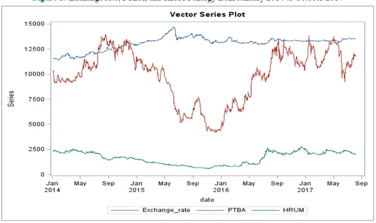
The data used in this study are HRUM energy and PTBA closing price, which were collected from January 2014 to October 2017 (LQ45a, 2018; LQ45b, 2018). The data Exchange Rate are also taken from January 2014 to October 2017 (Bank Indonesia, 2018). The data HRUM energy and PTBA are adopted from LQ45, and the Exchange Rate is adopted from the Bank Indonesia. The plot
of these data is given in Figure 1.
From Figure 1, it can be seen that the data for Exchange rate,
PTBA, and HRUM energy are nonstationary. The data for PTBA from January 2014 to October 2015 show an increasing trend, those from October 2015 to January 2016 show a decrease; in the data from January 2016 to September 2016 the trend still decreases, and from September 2016 to October 2017 the trend is flat, but with significant fluctuations. The data for HRUM energy from January 2014 to January 2016 shows a decreasing trend; for the data from January 2016 to September 2016 the trend increases, and from September 2016 to October 2017 the trend is flat, but with fluctuations. The data for the Exchange Rate from January 2014 to May 2015 shows an increasing trend, which slowly decreases and fluctuates from May 2015 to May 2016; this trend is finally flat from May 2016 to October 2017. Data analysis conducted using the ADF test shows nonstationary data (Table 1). The next step is to differentiate the data to make
them stationary in mean. Figure 2 shows the data obtained after
differentiation with d = 1.
By differentiation with d = 1, the HRUM energy and PTBA data become stationary. To find the best model, several models, namely, VARX (1) – VARX (5), were compared and the information criteria AICC, HQC, AIC, and SBC were used. The best fit was
correlated with the smallest values of those criteria, which are listed in Table 2.
Based on the values in Table 2, it is found that the best model is VARX (1,0), with the minimum value of SBC of 18.873. According to the HQC criteria, the best model is VARX (3,0), with a minimum value of 18.8516. The AICC and AIC criteria indicated VARX (4,0) as the best model, with minimum values of
18.8140 and 18.8136, respectively. The schematic representation
of parameter estimates for the VARX (1,0), VARX (3,0), and
VARX (4,0) models are given in Table 3.
According to the data in Table 3, three parameters (AR1) are significant in the VARX (1,0) model, and six parameters (AR1−3) are significant (sign: – and +) in the VARX (3,0) and VARX (4,0) models. Because no parameters are significant in AR4, model VARX (3,0) is used as the best model for the data.
Model VARX (3,0) is expressed by the following equation.
Γt = Γt
Table 1: ADF test for data PTBA and HRUM Energy before and after differentiation (d=1)
Variable Type Before differentiation After differentiation (d=1)
Rho P value Tau P value Rho P value Tau P value
PTBA Zero mean −0.17 0.6448 −0.21 0.6111 −1088.4 0.0001 −23.32 <0.0001 Single mean −4.74 0.4605 −1.50 0.5357 −1088.5 0.0001 −23.31 <0.0001
Trend −4.89 0.8286 −1.54 0.8159 −1089.3 0.0001 −23.30 <0.0001
HRUM Energy Zero mean −0.57 0.5561 −0.67 0.4272 −1003.0 0.0001 −22.37 <0.0001
Single mean −3.21 0.6313 −1.35 0.6065 −1003.2 0.0001 −22.36 <0.0001
Trend −3.64 0.9068 −1.53 0.8199 −1009.5 0.0001 −22.42 <0.0001
ADF: Augmented Dickey Fuller test
Table 2: Comparison of the criteria for VARX (1,0)–VARX (5,0) models
Information criteria VARX (1,0) VARX (2,0) VARX (3,0) VARX (4,0) VARX (5,0)
AICC 18.8360 18.8401 18.8202 18.8140* 18.8187
HQC 18.8517 18.8637 18.8516* 18.8531 18.8656
AIC 18.8359 18.8400 18.8199 18.8136* 18.8181
SBC 18.8773 18.9022 18.9029 18.9174 18.9427
Figure 1: Exchange rate, PTBA, and HRUM energy from January 2014 to October 2017
Figure 2: Residual plot, ACF, PACF, and IACF after differentiation with d = 1 for (a) PTBA and (b) HRUM energy data
Γ1t = 169.505 + 0.962 Γ1t−1 − 0.039 Γ2t−2 − 0.039 Γ1t−2 – 0.68 Γ2t−2
+ 0.061 Γ1t−3 + 0.777 Γ2t−3 – 0.001 Ψt + ɛ2t (18)
And
Γ2t = 22.929 − 0.005 Γ1t−1 + 1.070 Γ2t−1 − 0.001 Γ1t−2 – 0.144 Γ2t−2
+ 0.0004 Γ1t−3 + 0.070 Γ2t−3 – 0.008 Ψt + ɛ1t (19)
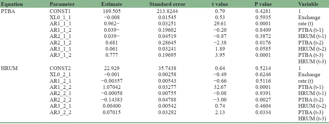
The statistical test results of the parameters in model (17) are
presented in Table 4, and those for models (18) and (19) are presented in Table 5. The results of the statistical test indicate
that model (18) is very significant, with the statistical test F = 12124.2 with P < 0.0001. The degree of determination, R-squared, is 0.9892. This means that 98.92% of the variation
of Γ1t (PTBA) can be explained by lag variables of Γ1t − 1, Γ2t − 1,
Γ1t − 2, Γ2t − 2, Γ1t − 3, Γ2t − 3 and Ψt (Exchange rate). According to the results obtained from the statistical test, model (19) is very significant, with the statistical test F = 25452.8 and P < 0.001. The degree of determination, R−Squared, is 0.9948. This means that
99.48% of the variation of Γ2t (HRUM Energy) can be explained
by the lag variables of Γ1t − 1, Γ2t − 1, Γ1t − 2, Γ2t − 2, Γ1t − 3, Γ2t − 3 and
Ψt (Exchange rate).
3.1. IRF
In economics, IRF is used to describe how economics reacts over time to the exogenous impulse, which economists usually call
shock and model in the context of VAR. Figure 3 shows the IRF
shock in exchange rate. One standard deviation in the exchange rate causes PTBA to respond negatively and increase up to 2 years.
The minimum effect occurs in lag 0 (the 1st day) with the value
about −0.007 and shifts to zero (stable condition) up to 2 years
(about 720 days (Figure 3a). Despite this, the negative impact of
PTBA is extremely small yet considerably significant in these
horizons until the 2nd year. The shock of one standard deviation in
the exchange rate also causes HRUM energy to respond negatively
and increase until the 2nd year (about 720 days). The minimum
effect occurs in lag 0 (the 1st day) with the value about −0.001 and
moves to zero (stable condition) up to 2 years (about 720 days
(Figure 3b). Even so, the negative impact on HRUM energy is very
small and close to zero yet highly significant in these horizons up
to two years. Figure 4a shows the impulse in PTBA. The shock of
one standard deviation in PTBA causes PTBA to respond positively and have significance for about 3 months, whereas from the third
up to the 7 month, the response moves to zero (stable condition).
Thus, the stable condition is reached up to the 7th month. It is
interesting to see the behavior of the confidence interval between
the third and 14th month when the volatility is high (Figure 4a).
The impulse in PTBA seems to have an effect on the volatility of
HRUM energy. Figure 4b shows that the HRUM energy is still
stable around zero when a shock in PTBA was noticed, but the
volatility is high up to one year after the shock in PTBA, which indicates that the closing price of HRUM energy fluctuates within one year following the shock in PTBA.
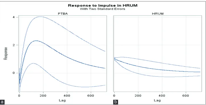
Figure 5a illustrates the IRF shock in HRUM energy. The shock
of one standard deviation in HRUM energy causes PTBA to Table 3: Schematic representation of parameter estimates
for the VARX (1,0), VARX (3,0), and VARX (4,0) models
Model Variable/lag C XL0 AR1 AR2 AR3 AR4
VARX (1,0) PTBA • • ++
Table 4: Statistical test for the parameters used in model (17)
Equation Parameter Estimate Standard error t value P value Variable
PTBA CONST1
Table 5: Univariate diagnostic checks
Model Variable R_squared Standard deviation F value P value
(18) PTBA 0.9892 269.11 12124.2 <0.0001
respond negatively for about 2 weeks; however, after that the impact is positive up to 2 years. The positive impact reaches
maximum in about the 5th month, then it decreases to zero (stable
condition) after 2 years (about 720 days). The impact is positive and very significant in the range of 2 weeks up to the 7 month because the confidence interval in this range does not include
zero (Figure 5a). From the behavior of the confidence interval
(Figure 5a), it can be observed that the volatility is very high.
Hence, it can be concluded that in this horizon, the closing price after the shock of HRUM energy fluctuates significantly. The impact of impulse in HRUM energy causes HRUM energy to respond positively and tend to zero in 2 years (about 720 days). Figure 3: (a and b) Impulse response function in exchange rate
a b
Figure 4: (a and b) Impulse response function in PTBA
a b
Figure 5: (a and b) Impulse response function IRF in HRUM energy
The impact up to the 6th month is positive and has significance
as zero is not included in the confidence interval. However,
from the 6th month up to 2 years, the impact is positive, but with
no significance as zero is included in the confidence interval
(Figure 5b).
3.2. Granger Causality
Table 6 shows that the Exchange rate does not induce Granger causality for PTBA and HRUM energy. The test is not significant with P value 0.7171 (>0.05). Yet, a null hypothesis is not rejected,
and this result that is in line with those displayed in Table 4, where
the XL0_1_1 and XL0_2_1 parameter, whose P values are 0.5935 and 0.6246, respectively, are not significant. In Table 6, Test 2 indicates that PTBA falls under the Granger causality for HRUM energy with P < 0.0001, whereas Test 3 shows that the HRUM energy does not obey the Granger causality rule for PTBA with P values of 0.8079.
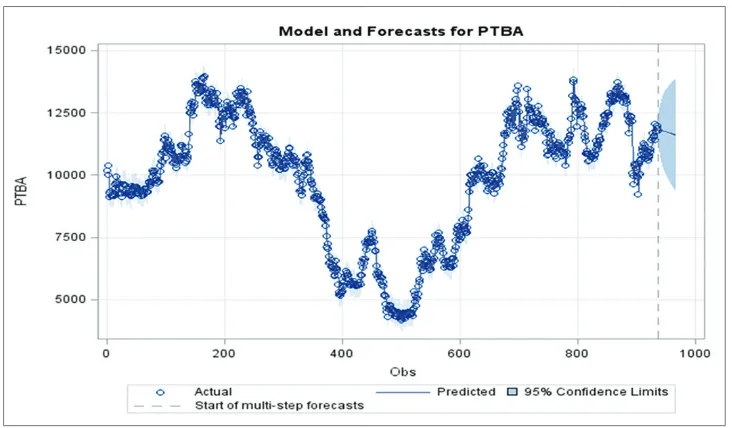
3.3. Forecasting
Forecasting is a process that allows the estimation of an unknown future value that is used in predicting the future values in a time
series of data. In this study, the VARX (3,0) model was used to forecast the 12 values (1 year prior) of PTBA and HRUM energy
data. Figure 6. A shows that the VARX (3,0) model for PTBA fits
very well with real data. The circle represents real data and the line represents the model. The predicted values and the confidence interval of 95% are given. Accordingly, the forecasting data of Figure 6: Prediction and forecasting of PTBA data
Figure 7: Prediction and forecasting of HRUM energy data
Table 6: Granger causality Wald test
Test Group DF Chi-square P value
Test 1 Group 1 variables: Exchange_rate
Group 2 variables: PTBA, HRUM 6 3.70 0.7171
Test 2 Group 1 variables: PTBA
Group 2 variables: HRUM energy 3 23.79 <0.0001 Test 3 Group 1 variables: HRUM energy
PTBA for the next 30 days seems to slightly increase. Figure 7
shows that the VARX (3,0) model for HRUM energy also fits very well with real data. As for the PTBA data, the circle represents the real values whereas the line represents the model. The predicted values and the confidence interval of 95% are given. It can be affirmed that the forecasting data of HRUM energy for the next 30 days also seems to increase.
4. CONCLUSION
Based on the results of the analysis of the relationship between the endogenous (PTBA and HRUM energy) and exogenous variables (Exchange rate), the VARX (3,0) model was found to be the best model for the relationship among these variables. The univariate models deduced from the VARX (3,0) model are very significant. On the basis of the IRF analysis, it was concluded that, if there is a shock in the Exchange rate, then the shock of one standard deviation in the Exchange rate causes PTBA and HRUM energy to
produce a negative response up to 2 years before reaching a stable
state (zero effect). Shock of one standard deviation in PTBA causes
PTBA to respond positively and attain a stable condition after the
7th month. It seems that the impulse in PTBA has an effect on the
volatility of HRUM energy; however, the HRUM energy is still
stable and close to zero when a shock in PTBA occurs. Shock of
one standard deviation in HRUM energy causes PTBA to respond negatively for about 2 weeks, but after that the impact is positive up to 2 years. The behavior of the confidence interval showed that
the volatility is very high.
Therefore, it can be concluded that in this horizon, the closing price after the shock of HRUM energy fluctuates greatly. The impact of impulse in HRUM energy causes HRUM energy to respond positively and tend to zero in 2 years.
5. ACKNOWLEDGMENTS
The authors would like to thank LQ45 Jakarta and Bank Indonesia for providing the data in this study. The authors would also like to thank Universitas Lampung for financially supporting this
study through Scheme Research Professor under Contract No:
1368/UN26.21/PN/2018. The authors would like to thank Enago (www.enago.com) for the English language review.
REFERENCES
Al-hajj, E., Al-Mulali, U., Solarin, S.A. (2017), The influence of oil price
shocks on stock market returns: Fresh evidence from Malaysia.
International Journal of Energy Economics and Policy, 7(5), 235-244. Bank Indonesia, Foreign Exchange Transaction Rates. Available from:
https://www.id.investing.com/currencies/usd-idr-historical-data. [Last retrieved on 2018 Feb 26].
Brockwell, P.J., Davis, R.A. (2002), Introduction to Time Series and Forecasting. 2nd ed. New York: Springer-Verlag.
Fuller, W.A. (1985), Nonstationary autoregressive time series. In: Hannan, E.J., Krishnaiah, P.R., Rao, M.M., editors. Handbook of Statistics. Vol. 5. Amsterdam: Elsevier Science Publishers. p1-23. Gourieroux, C., Monfort, A. (1997), Time Series and Dynamic Models.
United Kingdom: Cambridge University Press.
Hamilton, H. (1994), Time Series Analysis. Princeton, New Jersey:
Princeton University Press.
Juselius, K. (2006), The Cointegrated VAR Model: Methodology and Applications. Oxford: Oxford University Press.
Kilian, L. (2011), Structural Vector Autoregressions. Ann Arbor: University of Michigan and CEPR.
Kirchgassner, G., Wolters, J. (2007), Introduction to Modern Time Series Analysis. Berlin: Springer-Verlag.
LQ45a, Data Historis Saham PTBA. Available from: https://www. seputarforex.com/saham/data_historis/index.php?kode=PTBA. [Last retrieved on 2018 Feb 25].
LQ45b, Data Historis Saham HRUM Energy. Available from: https://www. seputarforex.com/saham/data_historis/index.php?kode=HRUM. [Last retrieved on 2018 Feb 20].
Lutkepohl, H. (2005), New Introduction to Multiple Time Series Analysis. Berlin: Springer-Verlag.
Pena, D., Tiao, G.C., Tsay, R.S. (2001), A Course in Time Series Analysis.
New York: John Wiley and Sons.
Sharma, A., Giri, S.S., Vardhan, H., Surange, S., Shetty, R., Shetty, V. (2018), Relationship between crude oil prices and stock market:
Evidence from India. International Journal of Energy Economics
and Policy, 8(4), 331-337.
Sims, C.A. (1980), Macroeconomics and reality. Econometrica, 48(1), 1-48.
Tsay, R.S. (2005), Analysis of Financial Time Series. New Jersey: John
Wiley and Sons, Inc.
Tsay, R.S. (2014), Multivariate Time Series Analysis. New Jersey: John
Wiley and Sons, Inc.