M ETH OD S
Valuing watershed quality improvements using conjoint
analysis
Stephen F arber
a,*, Brian G riner
baGraduate S chool of Public and International A ffairs, Uni6ersity of Pittsburgh, Pittsburgh, PA 15260, US A
bA ngus R eid Group,1700 Broadway, N ew Y ork, N Y 10019, US A
R eceived 25 October 1999; received in revised form 31 January 2000; accepted 1 F ebruary 2000
Abstract
This paper reports on a study of valuation of multiple stream quality improvements in an acid-mine degraded watershed in Western Pennsylvania. A technique extensively used in marketing research, conjoint (CJ) analysis, is used in conjunction with a random utility model (R U M ) to establish shadow valuations for various combinations of stream quality improvements in two streams. The technique shows promise in the valuation of ecosystems, which provide a complex variety of services. Several variations on respondent choice, binary choice (BC) and intensity of preference (IP) were used, where the latter allowed for an expression of degree of preference between status quo and alternative conditions. The sample constituted a panel data set from which user and non-user valuations were distinguished. In addition, sample respondents were identified by the distances of their residences to the stream sites, permitting the analysis of effects of distance on quality improvement valuations. These valuations suggested that persons living within roughly 50 miles of the evaluated stream segments place some positive value on stream improvements. © 2000 Elsevier Science B.V. All rights reserved.
Keywords:Conjoint; Valuation; Watersheds
www.elsevier.com/locate/ecolecon
1. Introduction
The purpose of this study is to employ a utility-theoretic based conjoint analysis (CJ) for valuing watershed quality improvements. While there are many examples of the use of CJ in marketing
(M cF adden, 1986; Louviere, 1988; Wittink and Cattin, 1989; G reen and Srinivasan, 1990), it has had limited use in economics. This is in spite of the fact that CJ estimating models are compatible with R andom U tility M odel (R U M ) formulations of choice (M cF adden, 1981). In the environmental area, CJ has been used to value water quality (Whitmore and Cavadias, 1974; Smith and D esvousges, 1986), visibility improvements in na-tional parks (R ae, 1983), diesel odor reductions
* Corresponding author. F ax:+1-412-6482605.
E -mail addresses: [email protected] (S. F arber), [email protected] (B. G riner)
(Lareau and R ae, 1989), preferences for siting municipal landfills (Opaluch et al., 1993), prefer-ences for various energy programs (Johnson and D esvousges, 1997), preferences for waterfowl hunting (M acK enzie, 1993), wild salmon manage-ment options (R oe et al., 1996), preferences for recreational activities (G an, 1992; Adamowicz et al., 1994), and values for protecting threatened woodland caribou populations (Adamowicz et al., 1998).
The purpose of CJ is to analyze choice in a multi-attribute context. Individuals are presented choice alternatives with varying values of at-tributes, and are asked to choose the best or rank/rate the alternatives. This hypothetical choice setting appears to mimic real choice set-tings in requiring the individual to simultaneously consider many dimensions of alternatives. The potential of CJ procedures for contingent valua-tions of ecosystems is direct. F irst, allowing one of the attributes to be a ‘price’ can be used to reveal implied valuations of individual attributes. Second, the multidimensional nature of the alter-natives allows a more realistic representation of complex ecosystems where a variety of dimensions may be important to individuals. Third, the choice is referendum-like and thereby emulates public decision situations.
CJ is defined as ‘‘any decompositional method that estimates the structure of consumer’s prefer-ences…given his or her overall evaluations of a set of alternatives that are prespecified in terms of levels of different attributes. Price typically is included as an attribute’’ (G reen and Srinivasan, 1990). As a general illustration of the CJ proce-dures, suppose we are interested in valuing a wetlands system and its component services. Sup-pose wetlands services include storm protection (S ), recreational fishing (F), and water treatment (W ). Let the utility level of the individual depend upon the level of these services as well as some price placed on the bundle of service, P. Then
U=f (S , F, W , P ). In particular, suppose that U=aS+bF+cW+dP, a general linear utility
function. CJ provides estimates of the ‘part-worths,’ a, b, c and d. In general, knowing these part-worths permits the valuation of any wetlands system since c/d, for example, measures the
mar-ginal value placed upon water quality treatment.
The CJ procedure establishes several levels of the attributes. F or example, S may be measured by the probability of a storm impacting the indi-vidual, and may have several values, say, 0.10, 0.20 and 0.30. R ecreational fishing service, F, may be measured by average fish catch per day, say, 0, 3, 6 and 10. Water treatment services may be simply measured by whether toxics are in the water, Yes or N o. Several prices may be used, say, $10, $50, and $100 per household per year. CJ then presents the respondent with combinations of the four attributes, and asks the respondent to select the best, to rank them or to provide a rating of them. In this example, there would be 3×4×
2×3=72 possible combinations of attribute lev-els. In order to simplify the choice, only a subset of these combinations would be used. Various software programs (e.g. SPSS Conjoint Ortho-plan) facilitate the selection of a reasonable num-ber of choice combinations. They typically select combinations that permit the estimation of only main effects. This is termed orthogonal design, and would not allow determining the interaction effects of, say, levels of W on P.
This paper reports on a study of watershed quality improvement for two streams in Western Pennsylvania, both degraded from acid mine drainage. CJ allows joint valuation of these poten-tially substitute goods. The study design includes distance from the two sites as a value-determining variable and allows determination of the spatial extent of the market for users and non-users. Several choice models were used to determine the sensitivity of valuation results to model specifica-tion. Section 2 outlines the experimental design, including the CJ design as well as survey questions and procedures. Section 3 derives the R U M -based estimation models, and Section 4 derives specific estimating equations. Section 5 presents the results of model estimation, including distinc-tions between user and non-user valuadistinc-tions. Sec-tion 6 is the conclusion.
2. Experimental design
Pennsyl-vania. This 2400 sq. mile watershed has a total of 3000 miles of stocked and natural freshwater streams providing opportunities for warm and cold water fishing. Also, some reaches permit boating and hiking. R oughly 15% of these stream miles are degraded, primarily from acid mine drainage (PA D EP, 1993). The sub-basins in which the two streams of interest are located, Loyalhanna Creek (subbasin 18C) and Cone-maugh R iver (subbasin D ), differ significantly in their extent of degradation. Loyalhanna Creek’s sub-basin has 60% of its stream miles degraded, and the Conemaugh R iver’s sub-basin has only 3% of its miles degraded.
H abitat evaluation by U S EPA and PA state fisheries biologists distinguishes between stream reaches that are Severely Polluted, M oderately Polluted and U npolluted. A Severely Polluted reach has been determined by biologists to be incapable of supporting fish and other organisms. F ishing conditions would be poor to non-existent. Wildlife could not rely on these streams for food and habitat. H owever, human health is not typi-cally affected. M oderately Polluted reaches will support only some fish and other organisms. R e-productive conditions for fish are poor, and fishing is supported but catch would be limited. U npolluted reaches are those where fish and other organisms can thrive. By these designations, Loy-alhanna Creek is currently M oderately Polluted and the Conemaugh R iver is Severely Polluted.
A mail survey was administered during the summer of 1996 to a sample of area residents. Individuals were presented with several choice scenarios and were asked to choose between the status quo and various combinations of stream quality improvements for the two streams. Each alternative had a price attached. A sample choice is shown below.
The survey used in this study is available from the authors. A brief letter presenting commonly asked questions and answers about water quality in the study region provided an introduction to the questionnaire. A map of the streams in the watershed, shaded according to the degree of degradation followed the introductory letter. A major difficulty was defining the ‘good’ for the choice alternatives. After discussion with fish and
wildlife managers, we decided to use a mixed habitat-fisheries characterization. The traditional water quality ladder (Smith and D esvousges, 1986) was not appropriate for the types of water quality improvements evaluated in this study. The resulting characterization of Severely Polluted, M oderately Polluted and U npolluted, based on survivability of fish and other organisms, was described to survey recipients. The areas of stream valuation were illustrated on the map provided. Instructions to recipients noted that stream clean-up would be costly, resulting in higher prices or taxes. Persons were asked to consider a price they would pay each year for the next 5 years.
The Loyalhanna Creek segment had two possi-ble quality conditions, M oderately Polluted and U npolluted; the Conemaugh R iver segment had three possible quality conditions, Severely Pol-luted, M oderately Polluted and U npolluted. The pilot and prior studies (Smith and D esvousges, 1986) suggested the use of five payment levels ($15, $45, $90, $180, $360). The policy issue in the watershed was a determination of valuation for stream quality improvements, so degradation of Loyalhanna Creek to Severely Polluted was not relevant. Consequently, there were a total of 25 possible alternatives to the status quo in the full choice set.
valuation of one stream improvement and the improvement in the other stream. H owever, we were interested in both the main and interaction effects; we wished to determine how the value of improving Stream A depended upon the improve-ment in Stream B. So we could not use an orthog-onal design. Instead, we opted to use a full binary choice design. Each respondent was given five choice sets, with prices varying across sets. There were five blocks of choice sets, with each block administered to one-fifth of the sample. An exam-ple of a single choice set for an individual is shown below:
The sampling design was to establish a 8×10 grid of cells, each 9 miles by 9 miles for a total of 6480 sq. miles, completely covering the Lower Allegheny Watershed and parts of adjacent water-sheds. Zipcodes were selected for each cell, with one, two or three zipcodes used for cells with more zipcodes included for cells closer to the streams of interest. Out of a total 460 possible zipcodes within the grid sampling area, 133 were selected for sampling and a commercial mailing database was used for selecting households. A pilot mail study of 200 persons resulted in a low response rate of 10% to the initial questionnaire. F ollow up phone calls suggested that a problem might have been complex instructions and choice, so the instruction and choice sections were modified to make them simpler.
A final sample of 3958 households was drawn and first class postage surveys mailed to them. Only one mailing was sent. A total of 510 house-holds responded, and 372 surveys were returned as undeliverable. This was only a 14% response rate, excluding undeliverables, which is low. H ow-ever, this rate is not far below that of other general population CJ samples (Adamowicz et al., 1994). Only 367 of the 510 returned surveys were usable as some respondents did not answer all valuation related questions, particularly income.
We undertook a phone survey of non-respon-dents after an initial mailing of 600 in order to examine reasons for non-response (M itchell and Carson, 1989). A total of 380 non-respondents were called. N early 20% had inoperable phone numbers. F orty percent stated that they had not received the survey or had misplaced it so a
second survey was sent to them. Twenty-five per-cent refused to participate in the phone interview. F ifteen percent, 56 households, had received the survey, had not returned it but did participate in the phone interview. Of these 56 households, 15 stated they were not interested in water quality issues or felt water quality was just fine. This does suggest a survey response bias, implying that val-uations derived from the survey responses may be overstated. Twelve of the 56 said they did not have time to fill out the survey. This response may also suggest a bias. Other reasons for non-re-sponse included ‘It was too confusing,’ ‘N ot ap-plicable to them,’ ‘D o not do surveys,’ or ‘Too old or sick to participate.’
The survey respondents’ characteristics differed slightly from the general population in the Lower Allegheny Watershed. The respondents were 68% male (compared to 48% in the watershed) and 99% white (compared to 96% in the watershed). The mean household size was 2.9 persons (com-pared to 2.6 persons in the watershed); mean age was 51 years (compared to 52 years in the water-shed); and median household income was $37 500 (compared to $30 100 for the sampling area). This suggests the sample is more male and higher income than the population. G eneralizing sample results to the population must consider these so-cio-economic differences, as well as the potential sampling non-response bias.
3. Econometric models
The basis for an econometric model is an indi-rect utility function implied by the choice of levels of consumption of n goods, including ecological services offered by streams. Individual i maxi-mizes the utility function:
Ui=U (xi, qi, ci); individual i=1,…,T (1)
subject to the budget constraint:
Ii−pixi+wi=0 (2)
where xi=xi1…xil…xin, vector of quantities of
goods, l=1,…,n; qi=qi1…qil…qin, vector of
qualities (i.e. characteristics) of goods, l=1,…,n;
characteris-tics, k=1,…,s; Ii, income; pi, vector of goods
prices, including stream visit costs; wi, exogenous
addition to income.
The indirect utility function is then:
Vi=V (pi, qi, ci, Ii+wi) (3)
R andom utility maximization (R U M ) (M cF ad-den, 1981) provides an empirical formulation for estimation of Eq. (3). Let an individual face a set of M discrete choices, j=0,…M , where the status quo is j=0 and j=1,…M are alternatives. The alternatives include various combination of the exogenous variables: goods quality, prices and incomes. U nder R U M the indirect utility function is partitioned into systematic and random, unob-servable components:
Vij=Vij+oij; i=1,…,T ; j=1,…,M (4)
where Vij is the systematic or predictable portion
of utility and oij is the random portion of utility.
The presence ofoijin the indirect utility function is
due to the inability to observe V . While we can observe elements entering into the systematic component, Vij, and predict, ex ante, which of the
alternatives, j=0,…,M , the individual will choose, prediction will not be perfect due to the presence of oij.
The difference in utilities between alternatives j and k is determined from Eq. (4):
(Vij−Vik)=(Vij−Vik)+(oij−oik) (5)
We cannot observe Vij−Vik directly, only its
sign. If the individual chooses j over k, Vij−Vik\
0. The probability this choice will be made is given by:
Pi, j\k=Pr[Vij−Vik\0]=Pr[oik−oijBV(ij−V(ik]
(6)
Assume a linear approximation to the system-atic component of V ,
Vij=z%ijgj+hij (7)
where hij is a fixed effect and z%ij the vector of
elements in Eq. (3). Letting y *i Vij−Vik, Vij−
Vik(z%ijgj−z%ikgk)+(hij−hik), oioij−oik, Eq.
(5) can be written:
y*i=x%ib+oi (8)
where x%
i=(1, z%ij, z%ik) and b=((hij−hik), gj, −
gk). Estimation ofbin Eq. (8) requires observable
values of y *i and an assumed error distribution for
oi.
3.1. Binary choice (BC)
U nder binary choice (BC), estimation of Eq. (8) requires defining (M cF adden, 1974):
yi=1 if y*i\0
yi=0 if y*i50 (9)
Therefore, Pr(yi=1)=Pr(−oiBx%ib)=F(x%ib),
where F( · ) is the cumulative distribution func-tion foroi. M cF adden (1974) has shown that when
oij is iid (Weibull), F( · ) is a logistic cumulative
distribution function. M aximum likelihood meth-ods can be used to estimate b in Eq. (8). One deficiency of using logit models to estimate coeffi-cients in Eq. (8) is that the relative probabilities of choosing between two choice alternatives are con-strained to be constant regardless of whether other alternatives are available. F or example, the relative probability of choosing a configuration of Stream A and B quality improvements relative to the status quo is independent of whether a third alternative, improving Stream C, is available. This condition is known as the Independence of Irrele-vant Alternatives (IIA), and can result in unrealis-tic probability estimates (Judge et al., 1985, p. 70).1
1The implications of IIA for the valuation estimates in this study can be considered. The procedure for valuation is to present the respondent with a binary choice, where Alternative 0 can be represented by (w0, A0, B0) and Alternative 1 by (w1,
When any element of zij is constant across
alternatives and the corresponding element ofgjis
also constant, the effect of that element on choice is not identifiable. H owever, a constant element of
zij may interact with other non-constant elements
requiring its inclusion in an interactive, or varying coefficients model (G riffiths et al., 1993). F or example, while income remains constant across choices, the effect of environmental quality im-provements on choice may depend on income.
The inclusion of hij in Eq. (7) allows for fixed
effects over individuals and alternatives. There may be a threshold of utility increase before an individual selects an alternative to the status quo. Letting j=0 represent the status quo, hi1−hi0=
hi\0. A more complex possibility of a fixed effect
arises from potential experimental design and elic-itation procedures. F or example, if respondents act as if the ‘right’ response is to choose the alternative to the status quo,hi\0. A fixed effect
could also be present if respondents have a desire for change (hi\0) or no change (hiB0). The
procedure for introducing fixed effects into the binary choice model has been developed by Chamberlain (1980, 1984) and Baltagi (1995). The procedure requires a panel data set, as in the present study, and conditions the likelihood func-tion on the summed 0, 1 responses across each individual’s revealed choices. F or example, the present study asked each respondent to make a choice in five different scenarios; the maximum conditioning value is then five.
4. Specific forms for estimation of shadow values
Let z%
ijrepresent a vector of attributes of
alter-native j presented to individual i, where zij=wij,
qij. Therefore, z represents a combination of
monetary payments and quality scenarios. Let pij,
cijand Iijbe defined as above and assume they are
constant for each individual across alternatives. A first-order approximation to V in Eq. (3) is:
Vij=z%ija+c%ijg+uIij+p%ijd+hij (10)
in this study holds p, c and I constant across alternatives, so estimating Eq. (8) becomes:
y*i=Dz%ia+Dhi+oi (12)
whereDzi%a=Dw%iaw+Dqi%aq. This formulation
al-lows for choice between alternatives j and k to depend upon the characteristics of those alterna-tives, w and q, as well as a fixed effect.
While p, c and I are constant across alternatives in the experimental design, they can potentially interact with alternatives to affect choice. This may be the case for income and distance from sites variables. D istance from an individual’s resi-dence to a site in the choice set, D, is a proxy for price of user access to the site. It may also reflect psychological distance from a site for non-users. While D may have a direct effect on V , it will not have a direct effect on DV . H owever, it may
interact with q, the environmental quality variable in the choice setting, to affect choice; for example, individuals further distant from a site whose qual-ity is improved would be less likely to value an improvement alternative than a person closer to the site. These interaction effects can be incorpo-rated by assuming:
aq=a¦q+ aDD+aII (13)
This formulation allows individual characteris-tics to interact with alternatives in determining choice. The resulting estimating equation is:
y*i=Dw%iaw+Dq%ia0+Dq%iaDD+Dq%iaII+Dhi+oi
(14)
The shadow value of a qualitative change, Dq,
can be obtained from the first-order approxima-tion to DV( i:
Dwi
Dqi
= −a0+aDDi+aIIi aw
(17)
the individual’s marginal valuation of a change in environmental quality, Dq.
5. Results
The Binary Choice (BC) estimation results for the R U M are shown in Table 1. While the exper-imental design allowed individuals to state an intensity of preferences for or against the alterna-tive to the status quo, the dependent variable used in BC estimates is coded 1 (yes) if the individual designates they would ‘probably yes’ or ‘definitely yes’ prefer the alternative to the status quo, and 0 (no) otherwise. The 0 response then includes
‘defin-itely not,’ ‘probably not’ and ‘maybe yes – maybe no’ responses. All estimations were performed using LIM D EP™ procedures.
The simplest BC model is shown in column 1 of Table 1. All signs are theoretically correct and highly significant in most cases. The implied mar-ginal valuation of an improvement in Stream A from M oderately Polluted to U npolluted (A: M
U ) is Dw/Dq1=0.2891/ −0.0076=$38.04. G iven
the phrasing of the choice question, this represents the respondent household’s willingness to pay each year for 5 years for this improvement. The corre-sponding value for improving Stream B from Severely to M oderately Polluted (B: SM ) is
$52.30 per household for each of 5 years; and the value for B: SU is $90.01. These marginal
valuations are shown in Table 3, column 1, along with the S.E. of the calculated values.
The set of choice alternatives was designed to permit testing of interaction effects of Streams A and B quality changes on each other; for example, to allow testing of whether an improvement in Stream B from S to M would depend upon whether Stream A was improved from M to U, or vice versa. U nfortunately, there was too much collinearity when these stream quality change interaction ef-fects were added to the basic model, and the LIM D EP statistical procedure would not converge. H owever, if Streams A and B, being in the same region, are strong substitutes, the valuation for B:
SU ($90.01) should equal the sum of valuations
of B: SM ($52.30) and A: MU ($38.04). This
is nearly true in the sample. The inability to assess stream quality interaction effects in the dataset means that we cannot confidently infer the value of one stream quality improvement independently of the quality conditions of the other stream.
The BC model for income interacting with the stream quality change variable is shown in Table 1, column 2. All signs are correct; higher incomes increase the likelihood of accepting a quality im-provement. A likelihood ratio test shows that the increase in Log (L ) with this specification is signifi-cant. Table 3, column 2, shows that this specifica-tion reduces marginal valuaspecifica-tions only slightly when evaluated at sample mean incomes. A simple ver-sion of the fixed effects BC model, which takes advantage of the panel-type data set, is shown in
Table 1
Estimation results for binary choice (BC) logit random utility modelsa
Coefficient for Basic Interactive F ixed effect (3)
variable (1) (2)
Constant −0.4156 −0.3959 na (0.02) (0.03)
aProbability values in parentheses; N=362.
Table 2
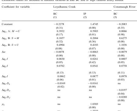
Estimation results for inclusion of distance variables in user BC and IP logit random utility modelsa Coefficient for variable Loyalhanna Creek Conemaugh R iver
IP
BC BC IP
(2) (3) (4)
(1)
1.4745 −0.2083 1.5110
−0.2278 Constant
(0.31) (0.00) (0.35) (0.00)
0.3932
Dq1, A: MU 0.5903 0.0066 0.2328
(0.17) (0.01) (0.98) (0.22)
0.2084 0.6275
Dq2, B: SM 0.1857 0.7368
(0.52) (0.36) (0.08) (0.01)
0.4103 1.1036 1.0660
0.4904
Dq3, B: SU
(0.08) (0.07) (0.00) (0.00)
Dw −0.0078 −0.0063 −0.0079 −0.0064
(0.00) (0.00) (0.00)
(0.00)
0.0807 0.0211
0.0261
Dq1·I 0.0830
(0.05) (0.42) (0.05) (0.51)
Dq2·I 0.0702 0.0541 0.0758 0.0602
(0.11)
(0.13) (0.13) (0.09)
0.0877 0.0978
Dq3·I 0.0862 0.0967
(0.06) (0.01) (0.03) (0.01)
Dq1·DL −0.0169 −0.0161 na na
(0.02) (0.00)
na −0.0197
na −0.0234
Dq2·DC
(0.04) (0.00)
na −0.0280
na −0.0291
Dq3·DC
(0.00) (0.00)
m2 na 1.0303 na 1.0414
(0.00) (0.00)
1.7727 na 1.7920
na
m3
(0.00) (0.00)
na
m4 2.9216 na 2.9525
(0.00) (0.00)
−1621.2 −618.4
−622.53 −1612.7
Log (L )
aProbability values in parentheses; N=217.
Table 1, column 3. The fixed effects model cre-ates a dummy-like variable for eachperson, repre-senting the sum of instances in which the individual selected rejected the status quo. A likelihood ratio test, with degrees of freedom be-ing the number of individuals in the estimatbe-ing sample, can be used to test the superiority of the fixed effects model. Such a test shows the fixed effects model to be a statistical improvement over either of the BC models. Table 3, column 3, shows that the estimated marginal valuations di-minish substantially for the fixed effects model compared to the other models. The purpose of
valuation estimates using the Basic and Interac-tive BC models are similar, and within 1 S.E. of each other. H owever, the estimated marginal val-uations using the F ixed Effects model, are nearly 1 S.E. lower than the other two BC model esti-mates. The estimated marginal valuations in columns 1 – 3, Table 3, all possess the property that the sum of the valuations for B: SM and
A: MU roughly equals the valuation for B: SU, which would be expected if streams A and
B are close substitutes.
The estimates for the IP models are not shown but are available from the authors. All coefficients are correctly signed and, except for the interactive model, were highly significant. Table 3 shows the IP marginal valuations to be higher than their BC counterparts. Apparently compressing the prefer-ence scale into two Yes/N o categories reduces valuation estimates. F or example, the marginal valuation for A: MU in the basic IP model,
column 4, is $50.02 per household for each of 5 years, compared to $38.04 in the BC model. The valuation estimates from the IP model are typi-cally at least 1 S.D . higher than the BC estimates. The F ixed Effects model continues to show lower valuation estimates than the Basic and Interactive models.
5.1. N on-user 6alues
The total value of water quality improvement is the sum of non-use and use valuations. One
means of operationalizing non-use values is to define valuations by persons who do not use the streams for any active or passive use as non-use values. This definition would implicitly include option values held by non-users. N on-use values held by users would not be estimated through this operationalization. We selected the subsample of households whose members did not use either of the two streams for any active or passive use during the year prior to the survey; they may or may not have used them prior to that time. The BC and IP models were estimated for this sub-sample of non-users.
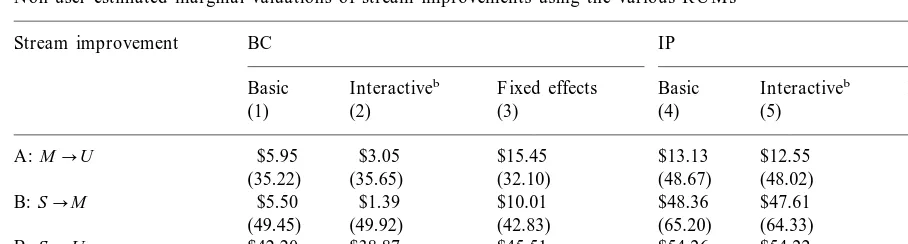
R oughly 25% of the sampled households did not make any visit to either of the two streams in the study. The estimated marginal valuations for the three types of quality improvements are shown by estimation model in Table 4 for the 70 non-user households. The estimated models are not presented in this paper, but are available from the authors. Table 4 suggests considerably lower valuations than those presented above for the total sample. In fact, none of the estimated valua-tions shown in this table are statistically signifi-cant, as shown by the large S.E. Valuations for stream A improvements, A: MU, ranged from
$3.05 to $15.45 per household per year for 5 years, depending upon the estimating model. Stream B improvements from severely to moder-ately polluted ranged from $1.39 to $48.36, de-pending on the estimating model. While the estimated valuations for the largest stream
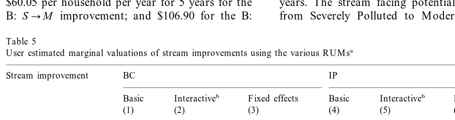
im-Table 3
Estimated marginal valuations of stream improvements using the various R U M sa
Stream improvement BC IP
Basic Interactiveb F ixed effects Basic Interactiveb F ixed effects
(5) (6)
(4) (3)
(2) (1)
$38.04 $38.59
A: MU $35.76 $26.63 $51.02 $51.35
(15.80) (15.89) (12.07) (17.17) (17.20) (9.27)
B: SM $52.30 $49.62 $35.90 $66.70 $67.64 $55.46
(21.40) (15.55) (22.85) (22.82)
(21.40) (11.97)
$90.01
B: SU $87.43 $75.63 $109.92 $112.44 $92.76
(21.78) (16.12) (23.10)
(21.80) (23.13) (11.90)
Table 1, col. 2
Table 4
N on-user estimated marginal valuations of stream improvements using the various R U M sa
Stream improvement BC IP
Interactiveb F ixed effects Basic
Basic Interactiveb F ixed effects
(1) (2) (3) (4) (5) (6)
A: MU $5.95 $3.05 $15.45 $13.13 $12.55 $5.17
(35.65) (32.10) (48.67)
(35.22) (48.02) (22.95)
$5.50
B: SM $1.39 $10.01 $48.36 $47.61 $28.50
(49.45) (49.92) (42.83) (65.20) (64.33) (30.40)
$38.87 $45.51 $54.26
$42.20 $54.22
B: SU $29.15
(49.41) (49.59) (43.62) (64.19) (63.42) (28.95)
aValues represent household willingness to pay for each of 5 years; S.E. ofDw/Dq in parentheses; N=70. Source: regressions not shown in paper, but are available from authors.
bEvaluated at sample mean household income.
provement, B: SU, ranging from $29.15 to
$54.22, are greater than for the other improve-ments, they are not statistically significant.
5.2. Use6alues
M odels were estimated separately for the 217 households that claimed to have members who used either of the two streams during the year prior to the survey. The marginal value estimates of users are shown in Table 5. The regressions that are the basis for these estimates are available from the authors. These estimated marginal valu-ations are highly significant, as the S.E. show. The BC models result in lower valuation estimates than the IP models. The fixed effects models result in lower values than the basic and interactive models. U ser values range from $23.09 to $53.56 per household per year for 5 years for the A:
MU change; from $39.93 to $70.63 for the B: SM change; and from $81.42 to $125.25 for the
B: SU change. U ser valuations in Table 5 are
generally higher than those in Table 3, the latter representing the total sample including non-users.
5.3. Distance effects on user and non-user 6aluations
D istance from an individual’s residence to stream sites would be correlated with the prices of use of those sites as well as psychological distance. Since distance remains constant across
alterna-tives in the choice set, a direct distance effect on choice cannot be identified. H owever, distance may have an interactive effect on choice insofar as it may diminish the desirability of stream im-provements. This would obviously be true of users of streams. But it also may be true for non-users, who may place existence or option values on stream quality improvements; a ‘sense of place’ may motivate individuals to value nearby quality improvements more highly in their ‘neighborhoods.’
A difficulty with testing distance hypotheses in this study is that the two streams under consider-ation are in close proximity, so any distances from a residence to each stream will be highly corre-lated. This limits the ability to analyze distance effects. D istance was measured using a G eo-graphic Information System which calculated straight line distances from the center of each respondent’s zip code to the nearest point of each stream.
non-use values have to be independent of space, otherwise they are use values in some form.
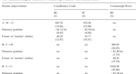
The distance effect should be more substantial for use values. Table 2 presents the model estima-tion results for the subsample of users. D istance to each stream is analyzed separately due to the high correlations of distances to the two streams. Columns 1 and 2 include the BC and IP estimates with the distance to Loyalhanna Creek. D istance has a significant negative effect when interacted with the quality change for that stream. M arginal valuation estimates for improvements to this stream are shown in Table 6. F or example, the BC estimate, evaluated at the subsample mean income and distance, is $45.36 per household per year for 5 years, which is comparable to the BC estimate for users in Table 5. Table 6 also shows a distance gradient for the BC estimate implying a decrease in marginal valuation of $2.15 per mile from this stream. The extent of the ‘market’ is defined as the distance at which the marginal valuation is zero, and is estimated to be 44.29 miles for this stream improvement. The IP model increases marginal valuations and the gradient.
Table 2 shows the estimation models including distance to the Conemaugh R iver interaction terms. The distance interaction effects are signifi-cant and negative. Table 6 shows the resulting marginal valuations for the two possible quality improvements for this river. The BC estimates are $60.05 per household per year for 5 years for the B: SM improvement; and $106.90 for the B:
SU improvement. The gradients are −$2.49 and −$3.54 per mile, respectively; and the ex-tents of the ‘market’ are 48.26 and 54.40 miles, respectively. It makes sense for the more substan-tial quality improvement to have a larger ‘mar-ket.’ The IP model estimates result in higher marginal valuations and gradients as well as smaller ‘market’ areas.
6. Conclusions
This study has used conjoint (CJ) procedures to obtain information for valuing stream quality im-provements in a watershed. A mail questionnaire was administered to a sample of households in Western Pennsylvania watersheds encompassing and surrounding two streams of interest. Potential stream quality improvements were characterized on the basis of habitat quality, and the house-hold’s ‘price’ of improvements was characterized as ‘$X per year for each of 5 years.’ R andom U tility M odel (R U M ) procedures were used to establish marginal valuations of quality improvements. The stream facing potential im-provement from M oderately Polluted to U npol-luted status, defined on the basis of habitat support value, resulted in valuations ranging from $26.63 to $51.35 per household per year for 5 years. The stream facing potential improvement from Severely Polluted to M oderately Polluted
Table 5
U ser estimated marginal valuations of stream improvements using the various R U M sa
Stream improvement BC IP
Basic Interactiveb F ixed effects Basic Interactiveb F ixed effects (5)
(1) (2) (3) (4) (6)
$46.77 $45.36 $23.09
A: MU $52.85 $53.56 $39.34
(19.70) (19.78) (14.74) (19.93) (19.99) (11.23) $62.91 $61.29 $39.93
B: SM $69.42 $70.63 $59.67
(26.67) (14.38) (26.39) (19.10) (26.69)
(26.41)
$125.25 $103.93
B: SU $110.35 $108.68 $81.42 $121.90
(27.22) (14.56) (27.13) (27.14) (20.06) (27.16)
aValues represent household willingness to pay for each of 5 years; S.E. ofDw/Dq in parentheses; N=217. Source: regressions not shown in paper, but are available from authors.
Table 6
U ser estimated marginal valuations of stream improvements with distance effectsa
Conemaugh R iver Loyalhanna Creek
Stream improvement
IP BC
BC IP
(2) (3)
(1) (4)
$52.46
A: MU $45.36 na na
(19.90) (19.68)
−$2.56/mi
D istance gradient −$2.15/mi na na
(0.94) (0.95)
43.71 na
Extent of ‘market’ (miles) 44.29 na
(10.51) (12.87)
na
B: SM na $60.05 $67.29
(26.05) (26.10)
na −$2.49/mi
D istance gradient na −3.69/mi
(1.19) (1.20)
na 48.26
Extent of ‘market’ (miles) na 42.41
(15.54) (8.83)
B: SU na na $106.90 $122.25
(26.80) (26.63)
na −$3.54/mi
na −$4.58/mi
D istance gradient
(1.21) (1.18)
na 54.40
na 50.88
Extent of ‘market’ (miles)
(12.52) (8.55)
aValues represent household willingness to pay for each of 5 years; S.E. ofDw/Dq in parentheses; N=217. Source, Table 2.
status showed valuations ranging from $35.90 to $67.64 per household per year for 5 years. The same stream exhibited valuations ranging from $75.63 to $112.44 per household per year for 5 years for potential improvement from Severely Polluted to U npolluted status. The study at-tempted to separately estimate non-user and user values. While not a perfect distinction, non-use and use were distinguished on the basis of whether members of a household visited either of the two streams during the year prior to the survey. M odel estimates for the small non-user group were poor and the resulting valuations were not statistically significant. Stream improvement values ranged from $1.39 to $54.26 per household per year for 5 years, depending on the improve-ment and estimating model. On the other hand, estimates for the user group were highly signifi-cant statistically. U ser valuations ranged from $23.09 to $125.25 per household per year for 5 years, depending on the improvement and esti-mating model. D istance from residence to each
stream had the expected negative effect on user valuations. The ‘extent of the market,’ defined as the distance beyond which marginal valuations for stream improvement became zero, ranged from roughly 45 to 55 miles, varying directly with the magnitude of quality improvement, as ex-pected.
streams, such as fishability, clarity and color, ve-locity, etc., and use CJ to hypothetically evaluate the part-worths, or marginal valuations, of each attribute. These part-worths could then be used to construct valuations for any quality improvement at any site. An advantage of CJ is its ability to provide these part-worth estimates. F inally, the experimental design only permitted binary choices. Other choice elicitations, such as ranking or rating, could result in very different valuations.
Appendix A. Intensity of preferences (IP) RUMs
The binary choice R U M can be extended to incorporate the intensity of preference for a choice using ordinal response categories. This model has been used by Bergstrom et al. (1982) to estimate demand functions for local school expen-ditures, M agat et al. (1988) to value morbidity risk reductions associated with chemical products, K amakura and Balasundaram (1993) to estimate the demand for electric utility products and ser-vices, and by Colias and Salazar-Velasquez (1995) to estimate purchase intent for new products. The estimation procedure is described here. Like the binary choice R U M , y * defined in Eq. (7) is unobservable. What is observed is:
yij = 0 if y*ijB0
= 1 if 05y*ijBm1
= 2 if m15y*ijBm2
·
·
= P−1 if mp−15y*ijBmp
= P if mp5y*ij
(A1)
where there are P+1 ordinal response categories and mp represents the unobserved threshold for
response category p. The single 0 threshold of the BC model is replaced by P thresholds in the IP model. A presumed advantage of permitting choice response intensities is that it may more accurately mimic mental heuristics in hypothetical choice situations, as opposed to real choice situa-tions where a 0, 1 choice is actually made. This
may lead to less rejection of the choice experi-ment; i.e. protest responses (R eady et al., 1995).
The probabilities of responses in each category are given by:
Prob[yij=0]=F(−xi%b)
Prob[yij=1]=F(m1−x%ib)
·
Prob[yij=P−1]
=F(mP−2−xi%b)−F(mP−1−xi%b)
Prob[yij=P ]=1−F(mP−1−x%ibb (A2)
where F is a cumulative distribution function (M cK elvey and Zavoina, 1975). The likelihood function follows directly from Eq. (A2). M axi-mum likelihood methods can be used to estimate (b, m).
References
Adamowicz, W., Louviere, J., Williams, M ., 1994. Combining revealed and stated preference methods for valuing envi-ronmental amenities. J. Environ. Econ. M anage. 26 (3), 271 – 292.
Adamowicz, P.B., Williams, M ., Louviere, J., 1998. Stated preference approaches for measuring passive use values: choice experiments and contingent valuation. Am. J. Agric. Econ. 80 (1), 64 – 75.
Baltagi, B.H ., 1995. Econometric Analysis of Panel D ata. Wiley, N ew York.
Bergstrom, T.C., R ubinfeld, D .L., Shapiro, P., 1982. M icro-based estimates of demand functions for local school ex-penditures. Econometrica 50 (5), 1183 – 1205.
Chamberlain, G ., 1980. Analysis of covariance with qualitative data. R ev. Econ. Stud. 47, 225 – 238.
Chamberlain, G ., 1984. Panel D ata. In: G riliches, Z., Intrilli-gator, M .D . (Eds.), H andbook of Econometrics. Elsevier, Amsterdam.
Colias, J.V., Salazar-Velasquez, C., 1995. Integrating the rank-ordered logit model with purchase intent survey questions for new products or services. Can. J. M arket. R es. 14, 46 – 56.
G an, C., 1992. A Conjoint Analysis of Wetland-Based R ecre-ations: A Case Study of Louisiana Waterfowl H unting, unpublished Ph.D . dissertation, D epartment of Agricul-tural Economics and Agribusiness, Louisiana State U niver-sity, Baton R ouge, LA.
G riffiths, W.E., H ill, R .C., Judge, G .G ., 1993. Learning and Practicing Econometrics. Wiley, N ew York.
Johnson, F .R ., D esvousges, W.H ., 1997. Estimating stated preferences with rated-pair data: environmental, health, and employment effects of energy programs. J. Environ. Econ. M anage. 34 (1), 79 – 99.
Judge, G .G ., G riffiths, W.E., H ill, R .C., Lutkepohl, H ., Lee, T., 1985. The Theory and Practice of Econometrics. Wiley, N ew York.
K amakura, W.A., Balasundaram, A., 1993. D esigning Innova-tive Products or Services With A R eservation-U tility M odel, working paper, K atz G raduate School of Business, U niversity of Pittsburgh.
Lareau, T.J., R ae, D .A., 1989. Valuing WTP for diesel odor reductions: an application of contingent ranking technique. South. Econ. J. 55 (3), 728 – 742.
Louviere, J.J., 1988. Conjoint analysis modeling of stated preferences. J. Transport Econ. Policy, January, pp. 93 – 119.
M acK enzie, J., 1993. A Comparison of Contingent Preference M odels. Am. J. Agric. Econ. 75, 593 – 603.
M agat, W.A., Viscusi, W.K ., H uber, J., 1988. Paired compari-son and contingent valuation approaches to morbidity risk valuation. J. Environ. Econ. M anage. 15, 395 – 411. M cF adden, D ., 1974. Conditional logit analysis of qualitative
choice behavior. In: Zarembka, P. (Ed.), F rontiers in Econometrics. Academic Press, N ew York, pp. 105 – 142. M cF adden, D ., 1981. Econometric models of probabilistic
choice. In: M anski, C., M cF adden, D . (Eds.), Structural Analysis of D iscrete D ata with Econometric Applications. M IT Press, Cambridge, M A.
M cF adden, D ., 1986. The choice theory approach to market research. M arket. Sci. 5 (4), 275 – 279.
M cK elvey, R .D ., Zavoina, W., 1975. A statistical model for the analysis of ordinal level dependent variables. J. M ath. Sociol. 4, 103 – 120.
M itchell, R .C., Carson, R .T., 1989. U sing Surveys to Value Public G oods: The Contingent Valuation M ethod. R e-sources for the F uture, Washington, D C.
Opaluch, J.J., Swallow, S.K ., Weaver, T., Wessells, C.W., Wichelns, D ., 1993. Evaluating impacts from noxious facil-ities: including public preferences in current siting mecha-nisms. J. Environ. Econ. M anage. 24 (1), 41 – 59. R ae, D .A., 1983. The value to visitors of improving visibility
at M esa Verde and G reat Smoky M ountain N ational Parks. In: R owe, R .D ., Chestnut, L.G . (Eds.), M anaging Air Quality and Scenic R esources at N ational Parks and Wilderness Areas. Westview Press, Boulder, CO. R eady, R .C., Whitehead, J.C., Blomquist, G .C., 1995.
Contin-gent valuation when respondents are ambivalent. J. Envi-ron. Econ. M anage. 29 (2), 181 – 196.
R oe, B., Boyle, K .J., Teisl, M .F ., 1996. U sing conjoint analy-sis to derive estimates of compensating variation. J. Envi-ron. Econ. M anage. 31 (2), 145 – 159.
Smith, V.K ., D esvousges, W.H ., 1986. M easuring Water Qual-ity Benefits. K luwer-N ijhoff, Boston.
SPSS, 1999. Conjoint Analyzer module.
Whitmore, G .A., Cavadias, G .S., 1974. Experimental determi-nation of community preferences for water quality-cost alternatives. D ecis. Sci. 5 (4), 614 – 631.
Wittink, D .R ., Cattin, P., 1989. Commercial use of conjoint analysis: an update. J. M arket. 53, 91 – 96.