www.elsevier.com / locate / econbase
Bias reduction in autoregressive models
*
K.D. Patterson
Department of Economics, University of Reading, Reading, Berks RG6 6AA, UK
Received 27 July 1999; accepted 16 December 1999
Abstract
It is well known that standard estimators of an AR(p) model are biased in finite samples, yet little is done in practice to remove the bias. Apparently small biases have important implications for the estimation of the impulse response function, which is a nonlinear function of the original coefficients. This note shows how to obtain estimators adjusted for first order bias based on Stine and Shaman’s fixed point characterisation of the bias (Stine, R.A., Shaman, P., 1989. A fixed point characterisation for bias of autoregressive estimators. Annals of Statistics 17, 1275-1284). 2000 Elsevier Science S.A. All rights reserved.
Keywords: First order bias; Impulse response; Bias reduction
JEL classification: C22
1. Introduction
It is well known that least-squares, Yule–Walker, and maximum likelihood estimators in autoregressive models are biased in finite samples. Consider the AR(1) model:
( yt2m)5a1( yt212m)1et (1)
Where m is the mean of the process and et is iid with 0 mean and constant variance. The first order bias, that is O(1 /T ) bias, of the least-squares estimator (LSE) is 2(2 /T )a1, if m is known and
2(113a1) /T, if m is unknown. With relatively small T and large a1, which are typical of macroeconomic time series, the first order bias could be quite large. The problem has been studied by, amongst others, Marriott and Pope (1954) and Kendall (1954), Orcutt and Winokur (1969), Bhansali (1981), Tjøstheim and Paulsen (1983) and Pantula and Fuller (1985). Shaman and Stine (1988) and Stine and Shaman (1989) derived the first order bias for least-squares (LS) estimation of a general
*Tel.:144-118-931-8159; fax: 144-1189-750-236. E-mail address: [email protected] (K.D. Patterson)
p-th order autoregression with known or unknown mean as a linear function of the unknown
autoregressive parameters. This paper argues that it is important not to ignore apparently small biases in least squares estimation, especially for estimation of the impulse response function. A simple to use procedure, based on the Shaman and Stine approach, is developed and its merits examined by means of a simulation study.
2. The impact of biases on the impulse response function
Since dynamic models are pervasive in modelling economic time series with finite samples one would expect the application of bias reduction methods to be more widespread than they are. Often first order biases are neglected in empirical work, with a possible reason for this being that the bias is not thought to be large. For example, with a150.95 and T580 in the AR(1) model, the first order bias, calculated as 2(113a1) /T, is 0.04813 or 5.07% of the true value. Whether or not this is ‘large’ or ‘small’ depends upon the purpose of the estimate. Whilst some might be willing to neglect this bias (which anyway depends on the unknown value ofa1, a point we address later) consider estimating the impulse response of a one-off one-unit shock at time t. To illustrate we compare takinga150.95 and
ˆ
a150.9520.0481350.9019 (assuming higher order bias terms are negligible). After h periods the
h ˆ h
true impact of the shock is (a1) , whereas the estimated impact is (a1) . For h510 anda150.95 this
ˆ
is 0.599, whereas fora150.9019 it is 0.356. The ratio of the latter to the former is 0.594, so that the apparently small bias quickly cumulates through the nonlinear impact response function, and the correct impact is underestimated by a factor of over 40% after ten periods. Another aspect of the same problem is that the estimated half-life of the shock is 13.51 periods for a150.95, but only 6.71
ˆ
periods for a150.9144 which substantially underestimates the ‘memory’ of the process.
3. Bias in least squares estimation
Following Marriott and Pope (1954) a number of authors have developed expressions for first order bias which depend upon the sample size and (unknown) parameters in the model. One of the most useful developments has been due to Shaman and Stine (1988) and Stine and Shaman (1989). They derive expressions of the bias to order 1 /T of the LSE in an AR(p) model and show that certain very particular finite order models are unbiased. These are projections of a unique (up to scale) infinite order process: the fixed point for a particular model order. If the time series is not generated by this process, the bias of least squares estimator pulls the estimator closer to the fixed point coefficients. We briefly outline this approach and then show how it can be operationalised. Whilst the method is illustrated with some low order examples, this is purely for expositional purposes as the method can be applied quite generally.
We consider the stationary AR(p) model. That is:
p
O
ai( yt2i2m)5et a0;1 (2)i50
21
ˆ ˆ ˆ ˆ ˆ
unknown. The LS estimator a;(1, a1, a2, . . . ,ap)9 ofa in Eq. (2) is a5(1, 2R r)9, where the elements of the estimated covariance matrix R are:
T known coefficients, and o(1 /T ) indicates terms of higher order than 1 /T. The term 2(B /T )p a is the first order bias vector. B comprises three matrices: Bp p5B1p1B2p1B . B3p 1p5diag(0, 1, . . . , p). B2p
The AR(p) model is usually written and estimated in the form:
p
The only modification required with the model written as in Eq. (3) is that after Bp has been computed, it is necessary to change the sign of the constant term in each bias expression; ai is now interpreted as defined by Eq. (3).
An example may help to show how the bias expressions are calculated. With p54, Bpa is:
(B1p 1 B2p 1 B )a3p 5 Bpa
Thus, for example, the first order bias in estimating a1, as in Eq. (3), by least-squares is
2(11a11a4) /T (Note the change of sign on the constant). Next it is helpful to define the bias for each of the i51, . . . , p, AR coefficients. Let b be the i-th row ofi 2B /T, with a change of sign onp
the constant term, then the bias in estimatingai is the scalar bia. The bias vector is the p31 column vector with bia in the i-th element.
p
Often interest centres on the long-run coefficient f; oi51ai rather than the individual lag
p
ˆ ˆ
coefficients. The least-squares estimator of the long-run coefficient isf; oi51aiwith first order bias
p
coefficients is slight, it can accumulate in estimatingf. For example, consider the AR(2) model with unknown mean, then the O(1 /T ) least-squares bias vector is (2(11a11a2) /T, 2(214a2) /T )9,
2
and the bias in estimatingf isoi51bia5 2(31a115a2) /T. For positivea1 anda2 the biases are reinforcing. For example, in the limiting casea2→1 (anda1→0 to ensure stability) then with T550 the bias→20.16.
4. Bias reduction
The expressions for first order bias are not operational because they depend on the unknown true values of the AR coefficients. Consider this problem in the AR(1) case, where apart from higher order
ˆ
terms, Eha1j2a15 2(113a1) /T. There are two possible solutions to this problem. The first
ˆ ˆ
apparently sensible one is to correct the bias by adding (113a1) /T to the least-squares estimatea1.
ˆ ˆ ˆ
The revised estimate is, therefore,a11(113a1) /T. This is not the best solution because as a1 tends to underestimate a1, the bias will also be underestimated. Suppose a150.9 and T550, and to
ˆ
illustrate assume no higher order biases so a150.826, then the revised estimate of a1 is 0.8261
0.06950.895, which is better than the first estimate but does not fully correct for the bias. The second
ˆ ˆ ˆ
procedure is due to Orcutt and Winokur (1969). Substitutea1 for Eha1j in Eha1j2a15 2(113a1) /
ˆˆ ˆ
T and solve for the unknown a1, which gives a15a1T /(T23)11 /(T23), where the solution is
distinguished by a double hat and referred to as the bias adjusted estimator, BAE. This procedure
ˆ
completely eliminates the bias for a1 taking its expected value.
This procedure can be generalised, but to ensure bias adjustment throughout advantage has to be taken of all first order unbiased coefficients. In obtaining the general form of the solution it is
ˆ
convenient to redefine the a vector to comprise just the p estimated coefficients, that is let
ˆ ˆ ˆ
starting with ap and by a simple re-ordering of a, D can be made a triangular matrix.2 As an illustration consider the AR(2) case. Then Eq. (4a) is:
This representation definest, D and D which can then be used in Eq. (4c) to obtain the solution for1 2
Note that the estimated standard errors of the bias adjusted estimators are the square roots of the
ˆ ˆ ˆ
ˆ ˆ ˆ ˆ
diagonal elements of the variance–covariance matrix of a, Var(a), where Var(a)5H[Var(a)]H9. Since in this case the LSE is minimum variance, a comparison in terms of mean square error, M.S.E., will not necessarily favour the BAE.
5. Simulation results
A number of simulation experiments were carried out to illustrate some key results. In particular how well does the BAE work in reducing total bias, especially for estimation of the long-run coefficient, and does a comparison in terms of M.S.E still favour the BAE?
2
The DGP was the stationary AR(2) model, yt5m1oi51ai( yt2i2m)1et with et niid(0, 1). The regression model treated the mean as unknown. Three sets of design parameters were chosen to typify different types of situation. In set 1, m50.1, a150.5, a250.4, so that the sum at 0.9 indicates the kind of long-memory process typical of macroeconomic time series. Second, m50.9, a15 20.3,
a250.4 and now the sum is at 0.1 is a long way from the unit circle. We would like to know not only that the bias adjustments work when they should but also that there is no or little adjustment if that is what is required. Hence, the third set ofm51.9, a15 20.4,a25 20.5 was chosen to be close to the fixed point where the least squares estimators are unbiased. All results are based on 30 000 replications.
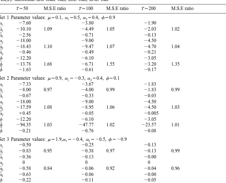
The results are summarised in Table 1. In each case, and for each coefficient, the first row entries refer to the theoretical first order bias for different sample sizes expressed as a % of the true value; the
ˆ
ˆ ˆ
second and third rows give the % mean bias for ai and ai, respectively. The M.S.E comparison is shown in the second column for each sample size, where the table entry is the ratio of the M.S.E of the LSE to the BAE for the individual coefficients and their sum.
With set 1 parameter values, the theoretical first order biases are relatively large, and typical of the kind of situation encountered with economic time series. For example, the first order bias is 27.6% fora1, 218% fora2 and 212.2% for the sumf. The mean biases for the LSE are close to but above
ˆ
these values. For example, with T550, the empirical (total) biases are: 210.1% fora1, 218.43% for
ˆ ˆ
a2 and 213.78% forf. These biases provide an estimate of the unaccounted for higher order biases that cannot be removed by using the (first order) bias adjustment. For example, fora1 the theoretical first order bias is27.6%, whereas the total bias is210.1%, the difference of 22.5% is attributable to
ˆˆ
higher order bias. The BAEs, ai, are effective in removing the first order bias. The M.S.E ratios are above 1, indicating that the reduction in the squared bias is not offset by the increase in the variance.
ˆ
ˆ ˆ
Table 1
AR(2): theoretical first order bias, LSE bias, BAE bias
T550 M.S.E ratio T5100 M.S.E ratio T5200 M.S.E ratio Set 1 Parameter values:m 50.1,a 50.5,1 a 50.4,2 f 50.9
a1 27.60 23.80 21.90
ˆ
a1 210.10 1.09 24.49 1.05 22.03 1.02 ˆˆ
a1 22.56 20.71 20.13
a2 218.00 29.00 24.50
ˆ
a2 218.43 1.10 29.47 1.07 24.70 1.04 ˆˆ
a2 20.46 20.49 20.21
f 212.20 26.10 23.05
ˆ
f 213.78 1.68 26.71 1.55 23.20 1.35
ˆˆ
a2 217.59 1.08 28.95 1.06 24.50 1.03 ˆˆ
a2 10.45 20.05 20.005
f 212.20 26.10 23.05
ˆ
f 294.35 1.03 247.77 1.02 223.57 1.01 ˆˆ
f 20.69 0.88 20.20 0.94 20.06 0.97
ˆˆ
f 20.50 20.09 20.00
the true value, whereas the BA estimate is 0.885. Even at T5100, a noticeable bias remains, with
ˆ
ˆ ˆ
mean f50.839, compared to mean f50.895. The estimated half-lives are 13.1 and 10.5 periods, respectively, compared to the true value of 9.3.
The picture is very similar for the second set of parameter values. The BAE removes the first order bias; for example, with T550, the first order bias is 27.33%, whereas the total bias is 28% with, therefore,20.67% accounted for by higher order terms. Because the biases ona15 20.3 anda250.4 work in the opposite direction algebraically, the sumf is very poorly estimated by LS. For example,
ˆ ˆ
for T550, mean a1 is 20.324 and mean a2 is 0.330, hence their sum is 0.06, whereas f50.1, and the response time to a shock is seriously underestimated; by contrast the mean of the bias adjusted sum is 0.0999. The gain in M.S.E terms is not quite as marked as with the first parameter set. There is no gain for estimating a1, but still a gain in estimating a2 and f.
the bias remaining in the BAE is in line with the estimate of remaining higher order bias. In this case the M.S.E comparison is now not favourable to the BAE compared to the LSE, with ratios below 1: because there is little bias to remove the (slight) increase in variance of the BAE is not outweighed by the bias reduction.
6. Conclusion
This note provides a simple operational procedure to compute (first order) bias-adjusted estimators and their standard errors based on the Shaman–Stine fixed point characterisation of bias. It argues that, for typical macroeconomic time series, bias adjustment is simple and worth doing in terms of total bias reduction and mean square error reduction, especially for the estimate of the long-run coefficient which otherwise cumulates the usually reinforcing bias from all component coefficients.
References
Bhansali, R.J., 1981. Effects of not knowing the order of an autoregressive process on the mean squared error of prediction. I. Journal of the American Statistical Association 76, 588–597.
Kendall, M.G., 1954. Note on the bias in the estimation of autocorrelation. Biometrika 41, 403–404. Marriott, F.H.C., Pope, J.A., 1954. Bias in the estimation of autocorrelations. Biometrika 41, 393–403.
Orcutt, G.H., Winokur, H.S., 1969. First order autoregression: inference, estimation, and prediction. Econometrica 37, 1–14. Pantula, S.G., Fuller, W.A., 1985. Mean estimation bias in least squares estimation of autoregressive processes. Journal of
Econometrics 27, 99–121.
Shaman, P., Stine, R.A., 1988. The bias of autoregressive coefficient estimators. Journal of the American Statistical Association 83, 842–848.
Stine, R.A., Shaman, P., 1989. A fixed point characterisation for bias of autoregressive estimators. Annals of Statistics 17, 1275–1284.