Directory UMM :Data Elmu:jurnal:J-a:Journal Of Applied Geophysics:Vol46.Issue1.2001:

www.elsevier.nlr_locater_jappgeo

AVO-A response of an anisotropic half-space bounded by a

dipping surface for P–P, P–SV and P–SH data

Luc T. Ikelle

a,)

, Lasse Amundsen

b

a

CASP Project, Department of Geology and Geophysics, Texas A & M UniÕersity, College Station, TX 77843-3115, USA

b

Statoil Exploration and Petroleum Technology Research Centre, USA

Received 20 October 1999; accepted 29 August 2000

Abstract

Ž .

We analyze amplitude variations with offsets and azimuths AVO-A of an anisotropic half-space bounded by a dipping surface. By analyzing the response of a dipping reflector instead of a horizontal one, we integrate the fundamental problem of lateral heterogeneity vs. anisotropy into our study. This analysis is limited to the three scattering modes that dominate

Ž .

ocean bottom seismic OBS data: P–P, P–SV and P–SH. When the overburden is assumed isotropic, the AVO-A of each of these three scattering modes can be cast in terms of a Fourier series of azimuths,f, in general form,

4

R _Žf_.sF q

_Ý

w

F cos nf_{Ž .}qG sin nf_{Ž .}

x

,

avoa 0 n n

ns₁

Ž .

where F , F and G are the functions that describe the seismic amplitude variations with offsets AVO for a given0 n n

azimuth. The forms of AVO functions are similar to those of classical AVO formulae; for instance, the AVO functions corresponding to the P–P scattering mode can be interpreted in terms of the intercept and gradient, although the resulting numerical values can differ significantly from those of isotropic cases or horizontal reflectors.

One of the benefits of describing the AVO-A as a Fourier series is that the contribution of amplitude variations with

Ž .

azimuths AVAZ is distinguishable from that of AVO. The AVAZ is characterized by the functions 1, cosf, sinf, cos2f,

4

sin2f, cos3f, sin3f, cos4f, sin4f, that are mutually orthogonal. Thus, the AVO–A inversion can be formulated as a series of AVO inversions where the AVO behaviors are represented by the functions F , F and G .0 n n

When the coordinate system of seismic acquisition geometry coincides with the symmetry planes of the rock formations, the series corresponding to P–P and P–SV simplify even further; they reduce to F for azimuthally isotropic symmetry and₀ to F , F , F , G and G for orthorhombic symmetry. The series corresponding to P–SH scattering is reduced to G and G0 2 4 2 4 2 4 for these two symmetries.

Unfortunately, the coordinate system of seismic acqusition geometry rarely coincides with the symmetry planes of the rock formations; therefore, the other terms are rarely zero. In particular, the functions F , F , G and G become important_{1 3 1 3} for large dips and are actually largely dependent on the angle of the dipping reflector. For P–P scattering, these functions are zero if the reflector is horizontal, irrespective of the anisotropic behavior. For P–SV and P–SH scattering, these functions

)

Corresponding author. Fax:q1-979-458-1513.

Ž .

E-mail address: ikelle@nutmeg.tamu.edu L.T. Ikelle .

0926-9851r₀₁r_{$ - see front matter}q2001 Elsevier Science B.V. All rights reserved.

Ž .

are not necessarily zero for horizontal reflectors because they are affected by the asymmetry of the P–S reflection in addition to the effect of dip.q2001 Elsevier Science B.V. All rights reserved.

Keywords: AVO-A; Ocean bottom seismic; Dipping surface

1. Introduction

Ž .

Ocean bottom seismic OBS data acquisition and processing system is a new oil and gas exploration and production tool that not only aims at remotely identifying fluid-saturated rock formations but also at determining their characteristics as well as any changes in their characteristics over time. These determinations are possible because OBS surveys have overcome three key limitations of

towed-Ž . Ž .

streamer surveys: i azimuthal coverage, ii

multi-Ž .

component recordings and iii repeatability of sur-veys. The 3D OBS can be designed with small enough spacing in both source and receiver coordi-nates to allow a full azimuthal coverage. Also, since it is carried out at the sea floor, three component

Ž .

particle velocity geophone data can be recorded

Ž .

along with pressure hydrophone data. This record-ing system gives us direct access to the shear-wave in addition to the P-wave. By considering a scenario where sensors are permanently placed at the sea floor, the repeatability of OBS is a realistic possibil-ity although some technological issues, such as the coupling of geophones to the sea floor, still remain to be overcome. To use these three new features of marine seismic measurements for retrieving fluid properties of rock formations, we need to gain more insight on how the physical properties which charac-terize fluid-saturated rocks are related to seismic data.

Fluid-saturated rocks contain small scale inhomo-geneities such as fractures that control the fluid flow in these rocks. At the scale of seismic wavelength, rocks containing these types of small scale inhomo-geneities behave as azimuthally anisotropic materi-als. Therefore, changes in the physical properties of such rock formations can produce amplitude

varia-Ž .

tions with offsets AVO as well as amplitude

varia-Ž .

tions with azimuths AVAZ . In short, we will call such amplitude variations AVO-A.

To identify and characterize fluid-saturated rock formations, we need to understand the correlations

between anisotropic parameters and AVO-A on one hand and the correlations between anisotropic pa-rameters and properties of fluid-saturated rock for-mations on the other. Such correlations make it possible to reduce the number of parameters in our inversion algorithms, which are generally ill-posed due partially to the large number of unknowns. These types of correlations can also help distinguish between different petrological models. Here we pre-sent an analysis of an AVO-A response to an anisotropic half-space bounded by a dipping surface as one way of improving our understanding of these correlations. The dipping surface can be planed or curved. By considering the response of a dipping reflector instead of a horizontal one, we have tried to integrate the fundamental problem of lateral hetero-geneity vs. anisotropy into our study. Our analysis will be limited to the three scattering modes which dominate OBS data: P–P, P–SV and P–SH.

We will use the weak-contrast assumption in our

Ž .

derivations i.e., Born approximation , but no weakly anisotropic assumptions are made of this material.

Ž .

We will consider transversely isotropic TI and orthorhombic symmetries as most experimental and theoretical studies suggest that the majority of rock

Ž

formations possess these symmetries e.g., Backus, 1962; White, 1975; Thomsen, 1986; Ikelle et al.,

.

1993; Sayers, 1998 . However, these symmetries are of interest in the derivations of AVO-A only if the axis of these symmetries coincides with the coordi-nate system of seismic acquisition geometries. Un-fortunately, the coordinate system of seismic acquisi-tion geometries sometimes does not coincide with the symmetry plane of rock formations. Even if they do coincide, such information is generally unknown. Our AVO-A analysis will show that the total anisotropic effect of reflection data can be described by a small number of simple linear combinations of the elastic stiffness tensor coefficients.

There are many publications on reflection

coeffi-Ž

1996; Zillmer et al., 1997, 1998; Ruger, 1998; Ursin

.

and Haugen, 1996; Vavrycuk and Psencik, 1998 .

˘

˘ ˘

The novelty here with respect to the previous works is that our derivations include the effect of a dipping reflector. We also produce mathematical constructs of AVO-A, which can be useful for AVO-A analysis and inversions by seeking the combinations of elastic parameters that best constrained P–P, P–SV and P–SH data. These mathematical constructs are

simi-Ž .

lar to those derived by Ikelle 1996 and

corrob-Ž .

orated by real data experiments Leaney et al., 1999 for P–P data when the acquisition plane is parallel to the dip direction.

A summary of the rest of this paper is as follows. In the next section, we will describe the basic elasto-dynamic properties of anisotropic media needed to introduce the general formulae of the AVO-A. We will also recall these formulae for the three scattering modes considered here. In the third, fourth and fifth sections, we will derive and analyze AVO-A formu-lae for each of the three scattering modes. Finally, in the sixth section, we will indicate the key pre-processing requirements for AVO-A inversion.

2. Introductory definitions

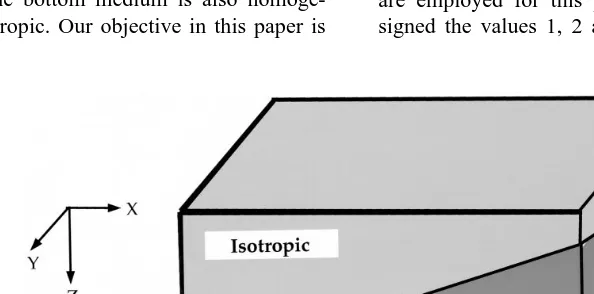
Consider two media separated by a dipping

inter-Ž .

face see Fig. 1 . The top medium, in which the sources and receivers are located, is homogeneous and isotropic; the bottom medium is also homoge-neous but anisotropic. Our objective in this paper is

to derive the AVO-A response of this configuration

Ž

under the weak-contrast approximation Born

ap-.

proximation . In this particular section, we introduce the basic definitions that we need for the AVO-A formulation.

The AVO-A formulation requires the slowness and polarization vectors which characterize the P-wave propagation from the source point to the scat-tered point on the dipping interface and those which characterize P- and S-wave upward propagation from the scattered point to the receiver point. As we have assumed that the top medium is homogeneous and isotropic, we are simply going to recall the well known analytic formulae of the slowness and polar-ization vectors for this particular case. We will also recall the compact definition of AVO-A on which our derivation will be based. To clarify the presenta-tion of these definipresenta-tions, we will start by introducing our notation convention.

2.1. Notations

Position in the configuration in Fig. 1 is specified

4

by the coordinates x, y, z with respect to a fixed Cartesian reference frame with the origin O and the

4

three mutually perpendicular base vectors i , i , ix y z

each of unit length. iz points vertically downwards. To accommodate anisotropy, the subscript notation for vectors and tensors and the Einstein summation convention are adopted. Lower case Latin subscripts are employed for this purpose; they are to be as-signed the values 1, 2 and 3 if not specified

wise. The lower case Latin subscripts s and r are reserved symbols for indicating source and receiver, respectively.

As we will see later, the quantities used to de-scribe AVO-A formulae depend on several variables. We will sometimes write these quantities without some of the variables when the context unambigu-ously indicates the quantity currently under consider-ation.

2.2. Vertical waÕenumbers, polarizationÕectors and slowness Õectors in an isotropic homogeneous medium

We start with the vertical wavenumbers corre-sponding to an isotropic, homogeneous, elastic medium. They are defined as follows for downgoing

Ž .

and for upgoing P- and S-waves to a receiver

loca-Ž . is the temporal frequency corresponding to time t; Õ_P andÕ_S are the P- and S-wave velocities of the top medium in Fig. 1, respectively. The vertical wavenumber qŽP. _{characterizes downgoing P-waves}

s

Ž .

propagating through the top medium see Fig. 1 from the source to the scattered point, and qŽP. _and

r

qŽS. _{characterize upgoing P- and S-waves} propagat-r

ing through the top medium from the scattered point to the receiver.

Let us now define the polarization vectors. The

˜

ŽP. ŽP._Ž X _.

and those of the upgoing P-, SV- and SH-waves are defined as follows:

Another set of vectors that we are going to need in the definition of AVO-A are slowness vectors.

ŽP. ŽP._Ž X _.

They are denoted by g

_˜

sg _{k , k ,s s} v _{for a} downgoing P-wave and defined as follows:

1 T

X X

ŽP. ŽP. ŽP.

g

_˜

sg

_Ž

_{k , k ,s s} v

_.

s _{k , k , qs s s .}

_{Ž .}

₈

v

For upgoing P-, SV- and SH-waves, they are defined as follows:

2.3. AVO-A for a weak-contrast interface

We can describe the materials in Fig. 1 by their density of mass, r, and their stiffness tensor, c_{i jk l}:

_rŽ0._{; c}Ž0._{4 characterizes the isotropic top medium}

while r _{, ci jk l characterizes the anisotropic} bot-tom medium. For an incident P-wave, the reflection at the interface between the two media produces three scattering fields: P–P, P–SV and P–SH. Under the weak-contrast approximation, the reflection coef-ficients characterizing the amplitude variations with

Ž

offsets and azimuths can be written see de Hoop et

.

al., 1994; Ikelle, 1996 :

Ž1.

˜

ŽP.

ˆ

ŽP.

˜

ŽP. ŽP.

ˆ

ŽP. ŽP.

for P–SV scattering

Ž

14

.

Ž3.

˜

ŽP.

ˆ

ŽSH. R_avoas b_i Drb_i

ŽP. ŽP. ŽSH. ŽSH.

˜

ˆ

q b_i g

_˜

_j Dc_{i jk l}b_k g

_ˆ

_{l ,}

for P–SH scattering

Ž

15

.

where

Alternatively, the tensorial stiffness Dci jk l will also be denoted by DC , respectively, where the sub-I J

scripts I and J run from 1 to 6, with ij™I accord-ing to 11, 22, 33, 23, 31, 12l1, 2, 3, 4, 5, 6.

Ž . Ž . Ž .

The Eqs. 13 , 14 and 15 are just alternative forms of small angle approximation of the reflection

Ž .

coefficients see Ikelle et al., 1992; Ikelle, 1995 . These formulae are derived from scattering theory assuming that density and stiffnesses are spatial step-functions. They do not use plane wave approxi-mation nor weak anisotropic approxiapproxi-mation.

How-Ž

ever, they assume a weak-contrast interface i.e.,

.

Born approximation .

Ž . Ž . Ž .

The effect of dip in Eqs. 13 , 14 and 15 is taken into account by the upgoing polarization and slowness vectors. As we will see later, the direction of the upgoing rays is modified if the interface is a dipping one instead of a horizontal one.

3. AVO-A derivation and analysis for P–P data

3.1. Dip and azimuthal angles

The amplitude variations with offsets and az-imuths RŽ1. _{for P–P scattering are given in Eq.}

avoa

Ž_{13 . To gain physical insight into R}. Ž1. _{, it is useful} avoa

to express it in terms of dip and azimuthal angles. This can be done by relating the wavenumbers k ,s

kXs, kr and kXr to incident and reflected angles as

re-flected ray and the vertical axis;f_{s is the azimuthal} angle between the x-axis and the line connecting the

Ž .

projection of the shot point in the plane x–y with that of the scattering point;f_{r is the angle between} the x-axis and the line connecting the projection of

Ž .

the receiver point in the plane x–y with that of the scattering point. These four angles are shown in

w

Figs. 2 and 3. The angles u_s and u_r vary over 0,

x w

pr_{2 ; the azimuthal angles} f_s and f_r vary over 0,

x

2p .

Alternatively, the anglesu_,uX_,f _and fX _{will be} used instead of u_s, u_r, f_{s and} f_{r. They are} intro-duced as follows:

ususyur,

Ž

22

.

uXsu_squ_r,

_Ž

₂₃

_.

f_sqf_r

fs _,

_Ž

₂₄

_.

2

f_syf_r X

fs _,

_Ž

₂₅

_.

2

whereu _{is the total reflection angle;} uX _{is the angle} of the dipping reflector; f _{is the azimuthal angle} between the x-axis and the plane containing the scattering point and midpoint; fX _{the azimuthal}

an-gle between the plane containing the scattering point and shot point and that containing the scattering point and receiver points. These four new angles are also shown in Figs. 2 and 3. As we can see in Fig. 2, uX _{is zero for the particular case where the reflector} is horizontal.

3.2. Decoupling of AVAZ and AVO

Ž . Ž . Ž .

By substituting Eqs. 18 – 25 in Eq. 13 and regrouping the different elements as a linear

nation of 1, cosf, sinf, cos2f, sin2f, cos3f,

4

sin3f, cos4f, sin4f , the amplitude variations with

Ž .

offsets and azimuths AVO-A can be cast in terms of a Fourier series of the azimuthal angle f as follows:

4

Ž1. Ž1. Ž1. Ž1.

Ravoas_F0 q

_Ý

_Fn _{cos n}

Ž

f

.

q_Gn _{sin n}

Ž

f

.

.

ns1

26

Ž

.

Ž1. Ž1._Ž X X_. Ž1. Expressions of functions F₀ s_F0 u_, u_,f _{, Fn}

Ž1._Ž X X_. Ž1. Ž1._Ž X X_.

s_Fn u_, u_, f _{and Gn} s_Gn u_, u_, f _{can be}

Ž

obtained from Table 1 the subscript n runs from 1

.

to 4 . Furthermore, the different elements of the

Ž .

series 26 can also be regrouped as a linear

combi-Ž .

Fig. 2. P–P reflection at an isotropicr_{anisotropic interface. a corresponds to a horizontal interface with,}us, the incident angle equal to,ur,

Ž .

Fig. 3. Azimuthal angles used in the radiation patterns for a case where the receivers are outside the acquisition plane.

from 0 to 4 can be deduced from Table 1.

The dependence of RŽ1. _{on f and f}X _describes avoa

Ž .

amplitude variations with azimuths AVAZ while its dependence on u and uX describes amplitude

Ž .

variations with offsets AVO . Thus, the AVO effect

Ž . Ž1.

in Eq. 27 of R_avoa is represented by the functions fŽ1._{, f}Ž1c._{, f}Ž1s._{, g}Ž1c._{, and g}Ž1s._{, all independent of}

0 m n m n m n m n m

the azimuthal angles f _and fX_.

Ž1. _{Ž .}

To simplify our analysis of Ravoa in Eqs. 26 and

Ž27 , we will limit our discussion to one azimuthal.

angle by taking fXs_{0 for the rest of this section} Ži.e., the source and receivers lie on the same line similar to when seismic data are arranged in

com-.

mon azimuthal sections, as described in Ikelle, 1996

Ž . Ž .

and we will use the series 26 instead of Eq. 27 . Ž1. Ž1._Ž X_. Ž1.

obtained from Table 1 by taking f s_{0 the} sub-.

script n runs from 1 to 4 .

Before we discuss the implication of these

con-Ž1. _{Ž .}

structs of R_avoa in Eq. 26 for an inversion algo-rithm, let us examine the AVO-A formula in Eq.

Ž26 for three symmetries regularly observed in ultra-. Ž

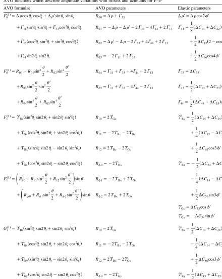
Table 1

AVO functions which describe amplitude variations with offsets and azimuths for P–P

AVO formulae AVO parameters Elastic parameters

Ž .

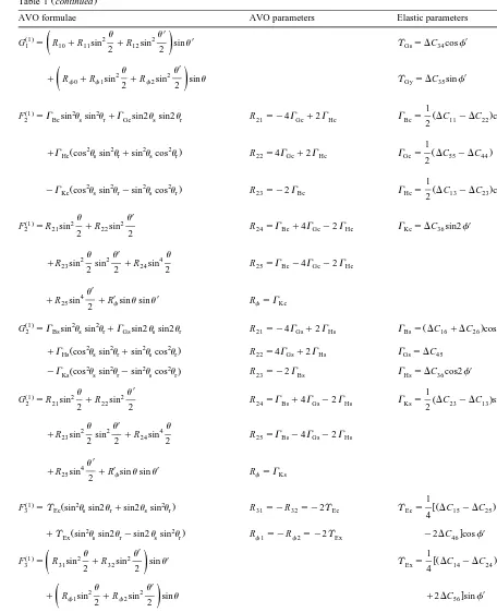
Table 1 continued

AVO formulae AVO parameters Elastic parameters

X

Ž .

Table 1 continued

AVO formulae AVO parameters Elastic parameters

X

Hornby, 1996 : transversely isotropic TI symmetry, orthorhombic symmetry and monoclinic symmetry.

Ž Ž ..

Using conditions Dc_{i jk l} see Auld 1990 , the

Ž .

AVO-A formula in Eq. 26 for TI media with

Ž .

respect to the vertical axis also known as TIV reduces to F1 _only:

0

RŽ1. _sFŽ1._{, 28}

Ž

.

avoa 0

which means that the amplitudes are invariant with azimuths. This result is consistent with the fact that the medium is azimuthally isotropic.

Let us now look at an example of azimuthally anisotropic media. For that, we consider an or-thorhombic medium. Using the conditions on Dci jk l

Ž

associated with orthorhombic symmetry see Auld

Ž1990 , the AVO-A formula in Eq. 26 is reduced.. Ž .

We can see that the amplitudes are no longer invari-ant with azimuths when medium perturbations are azimuthally anisotropic.

For the third example, we consider monoclinic symmetry. The conditions on D_{ci jk l associated with}

Ž .

monoclinic symmetry can be found in Auld 1990 .

With these conditions, the AVO-A formula in Eq.

Ž26 is reduced to.

A widespread concern in the interpretation of AVO-A response is the ambiguity between hetero-geneity and anisotropy. By deriving our AVO-A

Ž .

formula in Eq. 26 for a dipping reflector instead of the usual horizontal one, we can provide some in-sight on how these two physical properties affect amplitude variations with offsets and azimuths. Let us start our discussion by assuming that the interface between the isotropic and anisotropic media is

hori-Ž X

zontal i.e.,u s_{0, in the formulae in Table 1}

Basically, the f_{- and 3} f_{-terms of the Fourier} series are zero irrespective of anisotropic symmetry. Therefore, the AVO functions FŽ1.

, GŽ1. , FŽ1.

and

1 1 3

GŽ1.

are direct indicators of the dipping effect.

3

For some particular anisotropic symmetries like azimuthally isotropic symmetry and orthorhombic symmetry, the AVO functions FŽ1._{, G}Ž1._{, F}Ž1. _and

1 1 3

Ž1. _{Ž . Ž .}

G₃ are zero, as we can see in Eqs. 28 and 29 . The question then becomes: how to identify the effect of dip in these cases? For orthorhombic sym-metry, we can use the function FŽ1. _{to identify the}

2

effect of dip. In fact, the AVO-A for orthorhombic symmetry is described by three AVO functions: FŽ1._,

0

FŽ1. _{and F}Ž1._{. We can notice from their expressions}

2 4

in Table 1 that they can be written in the form of classical AVO formulae. For instance, FŽ1.

and FŽ1.

The definitions of the other parameters are given in Table 1. Using AVO terminology, we remark that AŽ1. _{and A}Ž1. _{are the intercepts for the AVO}

func-0f 2f

tions FŽ1. _{and F}Ž1._{, respectively; and B}Ž1. _{and B}Ž1.

0 2 0f 2f

are the gradients for the AVO functions FŽ1. and

0

FŽ1.

, respectively. We can also notice that the

inter-2

cept of FŽ1._{, which is A , is zero for the particular}

2 2f

Ž X .

case where the interface is horizontal i.e., us_{0 .}

Therefore, the value of the intercept of FŽ1. _{is a} 2

direct indicator of the dipping effect for orthorhom-bic symmetry.

The latest indicator of the dipping effect is based on the AVO function FŽ1.

which is zero for

az-2

Ž .

imuthally isotropic symmetry as shown in Eq. 28 . Hence, how can we recognize the dipping effect for this commonly used model of anisotropy? For this

Ž .

case, the series in Eq. 26 is reduced to AVO variations only, and it is described by FŽ1. _{only. As}

0

Ž . Ž1.

expressed in Eq. 32 , the intercept A_0f and gradient BŽ1. _{of F}Ž1. _{vary with the angle of the dipping}

0f 0

reflector in such a way that other equations with similar parameters are needed to distinguish the dip-ping effect. By combining the AVO FŽ1. _{of P–P}

0

with that of P–SV, we will later see that it is possible to identify the dipping effect even for az-imuthally isotropic symmetry.

Let us make another important remark about the AVO function FŽ1.

. If we assume that the bottom

0

medium in Fig. 1 is also isotropic, the intercept and

Ž1. _{Ž . Ž .}

gradient of F0 , defined in Eqs. 34 and 35 , are independent of uX_{, irrespective of the shape of the} interface between the isotropic and anisotropic me-dia, i.e.,

Therefore, in isotropic cases, the AVO of a dipping interface has the same form as that of a horizontal interface. This conclusion is generally translated by a statement such as: Athe AVO is a 1D effectB. Let us emphasize that this statement is only correct if the media under consideration are isotropic.

3.4. AVO-A analysis for inÕersion purposes

Basically, we would like to organize the

parame-ters Dr _and Dci jk l into combinations that are as

Ž . Ž .

Fig. 4. The AVO-A of P–P. The anisotropic materials used here are given in Table 2. a and b correspond to the orthorhombic material in

Ž . Ž .

Table 2a for a horizontal reflector and a 308dipping reflector, respectively. c and d correspond to the arbitrarily anisotropic material in Table 2b for a horizontal reflector and a 308dipping reflector, respectively.

on RŽ1. _{. These two important issues are discussed} avoa

in this section.

The dependence of RŽ1. _{on f describes} ampli-avoa

Ž .

tude variations with azimuths AVAZ while its de-pendence onuanduX describes amplitude variations

Ž .

with offsets AVO . Thus, the AVO effect in Eq.

Ž_{26 of R}. Ž1. _{is represented by the functions F}Ž1._,

avoa 0

FŽ1. _{and G}Ž1._{, which are all independent of the}

n n

azimuthal angle f_{. The AVAZ effect in this} equa-tion is represented by the trigonometric basic

tions 1, cosf_{, sin}f_{, cos2}f_{, sin2}f_{, cos3}f_{, sin3}f_,

4

cos4f_{, sin4}f _{. We can see that the AVAZ effect on} seismic amplitudes can be decoupled from the AVO

effect. Furthermore, we remark that the trigonomet-ric functions describing the AVAZ effect are mutu-ally orthogonal. This AVAZ property suggests that the AVO functions FŽ1._{, F}Ž1. _{and G}Ž1. _{can be}

ex-0 n n

tracted and processed separately based on the follow-ing equations:

2p

X X

Ž1. Ž1.

F0

Ž

u,u

.

s

_H

_Ravoa

Ž

u,u ,f

.

df,

Ž

42

.

0

2p

X X

Ž1. Ž1.

F_n

_Ž

u_,u

_.

s

_H

_Ravoa

_Ž

u_,u _,f

_.

_{cos n}f_df_, 0

Table 2

Ž . Ž . Ž .

Normalized stiffness tensorD_{ci jk l. a The anisotropic material used here is an orthorhombic rock as described by Cheadle et al. 1991 . b} We have rotated it to simulate the case where the axes of the symmetries do coincide with the coordinate system of the acquisition geometry

Ž .a

Parameter D_C11 D_C22 D_C33 D_C44 D_C55 D_C66 D_C12 D_C13 D_C23 Dr Value 0.4211 0.2578 y_0.0488 y_0.0655 y_0.0344 y_{0.0044 0.2500 0.2133 0.1844 0.1}

Ž .b

Parameter DC11 DC22 DC33 DC44 DC55 DC66 DC12 DC13 DC23

DC14 DC15 DC16 DC24 DC25 DC26 DC34 DC35 DC36

DC₄₅ DC₄₆ DC₅₆ Dr

Value 0.2546 0.3045 y0.0025 y0.0338 y0.0498 y0.0213 0.27037 0.1995 0.2144 y0.0251 0.0354 y0.0045 y0.0697 0.0184 y0.0369 y0.0565 0.0323 y0.01291 y0.0138 0.0191 y0.0228 0.1

2p

Another advantage of inverting each of these func-tions separately is that we significantly reduce the number of parameters to be estimated in each case. Before we discuss this point further, let us examine the contribution of these AVO functions to the AVO-A, RŽ1.

. We have plotted in Fig. 4 the AVO-A

avoa

for P–P scattering corresponding to the two models described in Table 2. We can see that small offsets behave as azimuthally isotropic media when the

Ž Ž1.

interface is horizontal i.e., F₀ is the dominant Ž1. _.

function in R_avoa . The presence of dip, which intro-duces the contributions of the functions FŽ1._{, G}Ž1._,

1 1

FŽ1. _{and G}Ž1._{, completely changes this pattern.}

3 3

Ž . Ž1.

Ikelle 1996 has suggested that the effect of F₃ , GŽ1._{, F}Ž1. _{and G}Ž1. _{might be small. The AVO-A in}

3 4 4

Fig. 5 computed without these terms shows that they are negligible, especially at small incident angles. This is an unfortunate outcome because the 3f- and

Ž

4f-terms involve single parameter inversion see

.

Table 1 ; therefore, they are easy to perform. How-ever, their extractions from RŽ1.

will be unreliable

avoa

for noisy data.

The inversion for parameters contained in the AVO functions FŽ1.

performed using classical AVO techniques. In fact,

Ž . Ž . Ž1.

we have shown in Eqs. 32 and 33 that F₀ and FŽ1. _{can be expressed in terms of the intercept and}

2

gradient just as in classical AVO. Actually, all these

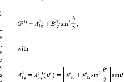
functions can be expressed in those terms; for in-stance, GŽ1.

in Table 1 can be rewritten:

1

The definitions of the other parameters are given in Table 1. Using AVO terminology, we remark that AŽ1.

and BŽ1.

are the intercept and gradient of the

1g 1g

AVO function GŽ1.

, respectively. With the AVO

1

Ž . Ž . Ž .

constructs in Eqs. 32 , 33 and 45 , we reduce the number of parameters to be inverted to two or three only.

u

Ž1. Ž1. Ž1. 2

q_B1gsinfq_{B2 fcos2}fq_{B2 gsin2}f

_.

_sin 2 u

Ž1. Ž1. Ž1. 4

q

_Ž

_{C0 f} q_{C2 fcos2}fq_{C2 gsin2}f

_.

_{sin ,} 2

48

Ž

.

and reduces to

u

Ž1. Ž1. Ž1. Ž1. Ž1. 2

R_avoas_{A0 f}q

_Ž

_{B0 f} q_{B2 fcos2}fq_{B2 gsin2}f

_.

_sin 2 u

Ž1. Ž1. Ž1. 4

q

_Ž

_{C0 f}q_{C2 fcos2}fq_{C2 gsin2}f

_.

sin , 2

49

Ž

.

when the interface is horizontal.

4. AVO-A derivation and analysis for P–SV data

4.1. Dip and azimuthal angles

Our task in this section is to derive and analyze the AVO-A for P–SV scattering. We will seek to utilize the AVO-A of P–SV to resolve some of the elastic parameters which cannot be recovered from P–P scattering alone.

As in the previous section, we will begin by relating the wavenumbers k , ks Xs, kr and kXr to incidence and reflecton angles as follows:

v

k_ss _sinu_scosf_s,

_Ž

₅₀

_.

Õ_P

Ž . Ž .

Fig. 5. The AVO-A of P–P where the 3f- and 4f-terms are dropped. The anisotropic materials used here are given in Table 2. a and b

Ž . Ž .

v X

kss _sinussinfs,

Ž

51

.

ÕP

v

k_rs _sinu_rcosf_r,

_Ž

₅₂

_.

Õ_S

v X

k_rs _sinu_rsinf_r.

_Ž

₅₃

_.

Õ_S

The angles f_{s and} f_{r are the same as those} intro-duced in Fig. 3. The angles u_{s and} u_{r are shown in} Fig. 6. Notice that, although these angles have the same meaning as those introduced in Fig. 2 for P–P, their physical behaviors are quite different. For in-stance,u_s is not equal to u_r even when the interface is horizontal, due to the asymmetry between P-wave and SV-wave reflections. However, they are related through Snell’s law:

Õ_P

sinu_ss _sinu_r.

_Ž

₅₄

_.

Õ_S

This relationship is only valid when the interface is horizontal because our angles,u_s andu_r, are defined with respect to the vertical axis and not with respect to the normal vector of the reflector.

Alternatively, the angles u, uX, f and fX will be used. They are introduced as follows:

usu_syu_r,

_Ž

₅₅

_.

uXsu_squ_r,

_Ž

₅₆

_.

f_sqf_r

fs _,

_Ž

₅₇

_.

2

f_syf_r X

f s _,

_Ž

₅₈

_.

2

whereu is the total reflection angle,uX is the angle due to the asymmetry between the P- and SV-wave reflection plus the dip angle of the reflector. The angles f and fX have the same meaning as those introduced in Fig. 3 for P–P scattering. The two new angles, u and uX, are also shown in Fig. 6. As we can see in Fig. 6, uX _{is non-zero even when the} reflector is horizontal, contrary to the P–P case.

4.2. Decoupling of AVAZ and AVO

As we did for P–P scattering, By substituting

Ž . Ž . Ž .

Eqs. 50 – 58 in Eq. 14 and regrouping the

ent elements as a linear combination of 1, cosf_,

Ž .

Fig. 6. P–SV reflection at an isotropicranisotropic interface. a corresponds to a horizontal interface. Contrary to the P–P reflection case,

Ž .

Table 3

AVO functions that describe amplitude variations with offsets and azimuths for P–SV scattering

AVO formulae AVO parameters Elastic parameters

1 X

Ž1. _{Ž .}

F₀ sDrsinu_scosu_ryDrcosu_ssinu_r R₀₀s DrqDrqG₃₃yG₁₃q2G₄₄ DrsDrcos2f 2

1 ₂ 1 1

Ž . Ž .

q G₁₁sinu_ssin2u_r R₀₁s y G₃₃qG₁₁ qG₁₃y₂G₄₄ G₁₁s D_C11qD_C22

2 2 8

1 ₂ 1 X

Ž . Ž .

y G₃₃cosu_ssin2u_r R₀₂s y_R04s G₁₁yG₃₃ =₂q_cos4f

2 2

1 1 1 X

Ž . Ž .

q G₁₃cos2u_ssin2u_r R₀₃s DryDryG₃₃qG₁₃q2G₄₄ q DC₁₂2ycos4f

2 2 4

1 1 1 X

Ž . Ž .

q G₄₄sin2u_scos2u_r R₀₅s G₃₃qG₁₁yG₁₃y2G₄₄ q DC₆₆cos4f

2 2 2

X

u u

Ž1. 2 2

F0 s

ž

R00qR sin01 qR02sin

/

sinu G33sDC33

2 2

X

u u X 1

2 2 _{Ž .}

q

ž

_R03q_{R sin}04 q_{R sin}05

/

_sinu G13s DC13qDC23

2 2 2

1 X

Ž .

G₄₄s D_C44qD_C55cos2f 2

1 1 X

Ž1. 2 _{Ž .}

F₁ sF_Bc

_ž

sinu_scos2u_rq sin2u_ssin2u_r

_/

R₁₀sF_GcqF_Gx F_Bcs DC₁₅qDC₂₅cosf

2 2

1 1 X

2 _{Ž . Ž .}

qF_{Gc cos}u_scos2u_ry sin2u_ssin2u_r R₁₃s4 R_f1s2F_BcqF_GcqF_BxqF_Gx q DC₁₅yDC₂₅cos3f

ž

2

/

4

1 1 X

2 _{Ž .}

qF_{Bx sin}u_scos2u_ry sin2u_ssin2u_r R₁₄s4yF_BxqF_Gx q DC cos3₄₆ f

ž

2

/

2

1 1 X

2 _{Ž . Ž .}

qF_{Gx cos}u_scos2u_rq _sin2u_ssin2u_r R₁₅s y₄F_BcyF_Gc F_Bxs y DC₂₄qDC₁₄sinf

ž

2

/

2

X

u u 1 1 X

Ž1. 2 2

Ž . Ž .

F₁ s_R10q_{R sin11} q_{R sin12 R11}s y _{2 R14}q_R13 y D_C14yD_C24sin3f

2 2 2 4

X

u u u 1 1 X

2 2 4 _{Ž .}

qR sin₁₃ sin qR sin₁₄ R₁₂s y 2 R₁₅qR₁₃ q DC sin3₅₆ f

2 2 2 2 2

X

u

X X

4

qR sin₁₅ qR_f1sinusinu F_GcsDC cos₃₅ f

2

X

F_Gxs yD_{C sin34} f

1 1 X

Ž1. 2

Ž .

G₁ sF_Bs

_ž

_sinu_scos2u_rq _sin2u_ssin2u_r

_/

R₁₀sF_GsqF_Gy F_Bss D_C14qD_C24cosf

Ž .

Table 3 continued

AVO formulae AVO parameters Elastic parameters

1 1 X

Ž .

Table 3 continued

AVO formulae AVO parameters Elastic parameters

4

sinf_{, cos2}f_{, sin2}f_{, cos3}f_{, sin3}f_{, cos4}f_{, sin4}f _, the amplitude variations with offsets and azimuths

ŽAVO-A can be cast in terms of a Fourier series of.

the azimuthal anglef _{as follows:}

4

obtained from Table 3 the subscript n runs from 1

.

to 4 . Furthermore, the different elements of the

Ž .

series 59 can also be regrouped as a linear

X X X X X

from 0 to 4 can be deduced from Table 3.

Just like for the P–P case, the dependence of RŽ2.

on f _and fX _{describes amplitude variations} avoa

Ž .

with azimuths AVAZ while its dependence on u and uX describes amplitude variations with offsets

Ž_{AVO . Thus, the AVO effect in Eq. 26 of R}. Ž . Ž1. _is avoa

represented by the functions fŽ2._{, f}Ž2c._{, f}Ž2s._{, g}Ž2c._.

0 m n m n m n m

We will limit the rest of our discussion in this section to one azimuthal angle by taking fXs_0,

Ž . Ž .

using the series 59 instead of Eq. 60 . Hence, the Ž2. Ž2._Ž X_. Ž2. Ž2._Ž

from Table 3 by taking f s_{0 the subscript n runs} .

from 1 to 4 .

Ž . Ž .

By comparing Eqs. 26 and 59 , we can remark that the AVAZ behavior of P–SV scattering has exactly the same form as that of P–P. This similarity

Ž .

is preserved for transversely isotropic TI , or-thorhombic and monoclinic symmetries. In fact, for

Ž .

TI symmetry with respect to the vertical axis TIV ,

Ž . 2

the AVO-A formula in Eq. 59 is reduced to F0

only:

RŽ2. _s FŽ2.

,

Ž

61

.

avoa 0

which means that the amplitudes are invariant with azimuths. For orthorhombic symmetry, we must add

Ž2. Ž2. _{Ž .}

the functions F2 and F4 to Eq. 59 :

RŽ2. _sFŽ2._qFŽ2._{cos 2f qF}Ž2._{cos 4f . 62}

Ž

.

Ž

.

Ž

.

avoa 0 2 4

For monoclinic symmetry, the AVO-A formula in

Ž .

Notice that 61 , 62 and 63 are similar to Eqs.

Ž28 – 30 , respectively.. Ž .

We have established that the structure of AVAZ of P–SV is similar to that of P–P. By comparing the third columns of Tables 1 and 3, we can also observe that the combinations of elastic parameters invoked in P–SV are exactly the same as those in P–P. The differences between P–P and P–SV are in their AVO behaviors. We will analyze these differences in more detail below.

4.3. Effect of dip

As discussed in the previous sections, the dipping and anisotropic effects on AVO-A of P–P scattering are distinguishable. However, the case where the

Ž .

bottom medium see Fig. 1 is azimuthally isotropic has not yet been resolved. The AVO function FŽ2. _of

0

Ž . Ž .

Fig. 7. The AVO-A of P–SV. The anisotropic materials used here are given in Table 2. a and b correspond to the orthorhombic material

Ž . Ž .

in Table 2a for a horizontal reflector and a 308dipping reflector, respectively. c and d correspond to the arbitrarily anisotropic material in Table 2b for a horizontal reflector and a 308dipping reflector, respectively.

Ž .

at normal incidence i.e., us_{0 . The definitions of} s

G₃₃ and G₁₃ are given in Table 3. If the interface is assumed horizontal, the reflected angle u_r is zero

Ž_{us0 whenever}. _{us0; thus, F}Ž2. _{is zero.}

How-r s 0

ever, if the interface is a dipping one as described in Fig. 1, u/_{0 even when} us_{0; hence, F}Ž2. _is

r s 0

non-zero. This remark can be used as a dip indicator for azimuthally isotropic symmetry.

Contrary to what we have seen for P–P scattering, notice that the functions FŽ2.

, FŽ2. , GŽ2.

and GŽ2. are

1 3 1 3

non-zero even if the interface is horizontal because uX/_{0 due to asymmetry between the P–SV}

reflec-tion.

4.4. AVO-A analysis for inÕersion purposes

The inversion procedure of AVO-A of P–SV is similar to that outlined earlier for P–P. We first extract the AVO functions FŽ2._{, F}Ž2. _{and G}Ž2. _from

0 n n

RŽ2. _{as follows:} avoa

2p

X X

Ž2. Ž2.

F0

Ž

u,u

.

s

_H

_Ravoa

Ž

u,u ,f

.

df,

Ž

65

.

0

2p

X X

Ž2. Ž2.

Fn

Ž

u,u

.

s

_H

_Ravoa

Ž

u,u ,f

.

cos nfdf,

0

2p

X X

Ž2. Ž2.

G_n

_Ž

u_,u

_.

s

_H

_Ravoa

_Ž

u_,u _,f

_.

_{sin n}f_df_, 0

for ns_1,2,3,4.

_Ž

₆₇

_.

Then, the problem is reduced to inverting each AVO function separately. From their definitions in Table 3, the maximum number of parameters to be inverted in each case is five.

In light of the observations made about the 3f -and 4f_{-terms of the Fourier series of P–P, let us} begin our discussion of the AVO inversions of P–SV by examining our capability to extract the AVO

functions FŽ2._{, G}Ž2._{, F}Ž2. _{and G}Ž2. _{from R}Ž2. _{. Fig. 7}

3 3 4 4 avoa

shows the AVO-A for P–SV scattering correspond-ing to the two models described in Table 2. We have repeated the same computations without these 3f -and 4f_{-terms in Fig. 8. We can see that the} contribu-tion of these terms is negligible. Based on several other tests that we have conducted, we have ob-served that these terms are usually small and can be dropped from the inversion process.

Our goal in AVO inversions of AVO functions for P–SV scattering is not to try to invert for all the parameters described in column 2 or 3 of Table 3, but rather to seek to improve the resolution of those

Ž .

Fig. 8. The AVO-A of of P–SV where the 3f- and 4f-terms are dropped. The anisotropic materials used here are given in Table 2. a and

Ž .b correspond to the orthorhombic material in Table 2a for a horizontal reflector and a 308_{dipping reflector, respectively. c and d}Ž . Ž .

Table 4

AVO functions that describe amplitude variations with offsets and azimuths for P–SH scattering

AVO formulae Elastic parameters

X

Ž3. 2

F₀ sDrsinu_sqG₁₁sinu_s sinu_rqG₄₄sin2u_s cosu_r DrsDrsin2f

1 1 1 X

G11s ŽDC22yDC11.y DC12q DC66 sin4f

8 4 2

1 X

Ž .

G₄₄s DC₄₄yDC₅₅sin2f 2

1 X 1

Ž3. 2

Ž . wŽ .

F1 sFBcsinus cosurqFGcsin2us sinur FBcs DC14qDC24cosfq DC14yDC24

2 4

1

X X

2 x Ž .

qF_Hccosu_scosu_r y₂D_C56cos3fq D_C15qD_C25sinf 2

1 X

wŽ . x

q DC₁₅yDC₂₅ q2DC₄₆sin3f 4

1 X

wŽ . x

F_Gcs DC₂₄yDC₁₄ q2DC₅₆cos3f 4

1 X

wŽ . x

q D_C15qD_C25 q₂D_C46sin3f 4

X X

F_HcsDC cos₃₄ fqDC sin₃₅ f

1 X 1

Ž3. 2 _{Ž .} wŽ .

G1 sFBs_sinuscosurqFGs_sin2us sinur FBss y DC15qDC25cosfq DC15yDC25

2 4

1

X X

2 _x

Ž .

qF_Hscosu_s cosu_r q2DC₄₆cos3fq DC₁₄qDC₂₄sinf 2

1 X

wŽ . x

q D_C24yD_C14 q₂D_C56sin3f 4

1 X

wŽ . x

F_Gss DC₂₅yDC₁₅ y2DC₄₆cos3f 4

1 X

wŽ . x

q DC₂₄yDC₁₄ q2DC₅₆sin3f 4

X X

F_HssDC sin₃₄ fyDC cos₃₅ f

1 X 1 X

Ž3. 2

Ž . Ž .

F₂ sG_Bcsinu_ssinu_rqG_Gcsin2u_scosu_r G_Bcs y DC₁₁qDC₂₂sin2fq DC₁₆qDC₂₆cos2f

4 2

2

qG_Hccosu_s sinu_r G_GcsD_C45

1 X X

Ž .

Ž .

which cannot be properly reconstructed from P–P alone. When possible, we will also seek to recon-struct parameters which cannot be solved from P–P at all. We have identified two such cases: one is related to the inversions of FŽ2._{, F}Ž2. _{and G}Ž2._{, the}

0 2 2

other is related to the inversions of FŽ2. _{and G}Ž2._.

1 1

Earlier we had seen that when the interface be-tween the isotropicr_{anisotropic media is horizontal,}

elastic parameters related to the f- and 3f-terms cannot be reconstructed from P–P scattering because the corresponding AVO functions are zero. Fortu-nately, these terms are not zero for P–SV scattering because of the asymmetry of P–SV reflection. Since

the combinations of elastic parameters invoked in

Ž

P–SV are the same as those in P–P see the 3rd

.

Further-u

where one of the two parameters can be extracted as

Ž X .

the intercept i.e., by taking usu s_{0 and the}

other by simply fitting the corresponding AVO curves. The definitions of F _, F _, F _and F

Bc Gc Bs Gs

are given in Table 4.

For dipping interfaces, we have seen that the parameters reconstructed from P–P, using the classi-cal AVO technique of the intercept and gradient, are dependent on the angle of the dipping reflector as

Ž Ž . Ž .

well as the elastic parameters see Eqs. 34 , 35 ,

Ž37 , 38 , 46 and 47 . We need other equations,. Ž . Ž . Ž ..

containing the same angle of the dipping reflector and the same elastic parameters, to extract the elastic parameters. The AVO functions FŽ2._{, F}Ž2. _{and G}Ž2.

0 2 2

of P–SV provide us these extra equations. We will consider these functions as normal incident cases just to make sure they are fully compatible with the angle definition introduced for P–P. At normal incident, the angle uXs yu _{is identical to the angle of the} dipping reflector. The AVO functions FŽ2.

, FŽ2.

Let us remark that, for the particular case where the anisotropic medium is considered isotropic, the AVO formula FŽ2._{, in Table 3, is reduced:}

Notice that this formula is independent of uX; it depends only on the total reflection angle between the downgoing P-wave ray and the upgoing SV-wave ray. Hence, the AVO effect can also be characterized in P–SV scattering as simply a A1D effectB if the

Ž .

overburden is isotropic because formula 74 is valid for a dipping reflecting interface. We can also notice that this formula is independent of compressional modulus.

5. AVO-A derivation and analysis for P–SH data

5.1. Dip and azimuthal angles

We now turn to the derivation and analysis of the AVO-A for P–SH scattering. The amplitude varia-tions with offsets and azimuths RŽ3.

for P–SH

avoa

Ž .

scattering are given in Eq. 15 . To gain physical insight into RŽ3. _{, we will express it in terms of dip}

avoa

and azimuthal angles. This will be done by using the definitions of the wavenumbers k , k_s X_s, k and k_r X_r as functions of incident and reflected angles given in

Ž . Ž .

Eqs. 50 – 58 .

Alternatively, the angles f _and fX _{will be used}

Ž .

instead of f_{s and} f_{r. They are defined in Eqs. 57}

Ž .

and 58 . Since the P–SH-wave is not polarized in the incidence plane, it is rather polarized along the y-axis. Hence, we did not find any benefit for using u _anduX _{instead of}u_{s and} u_r.

5.2. Decoupling of AVAZ and AVO

As we did for P–P scattering, by substituting Eqs.

Ž58 – 61 in Eq. 15 and regrouping the different. Ž . Ž .

elements as a linear combination of 1, cosf_{, sin}f_,

4

cos2f_{, sin2}f_{, cos3}f_{, sin3}f_{, cos4}f_{, sin4}f _{, the} amplitude variations with offsets and azimuths

ŽAVO-A can be cast in terms of a Fourier series of.

the azimuthal angle f _{as follows:} 4

Žthe subscript n runs from 1 to 4 . Furthermore, the.

Ž .

X X

regrouped as a linear combination of cosf_{, sin}f_,

X X X X X X

We will limit the rest of our discussion in this section to one azimuthal angle by taking fXs_{0 and}

Ž . Ž .

we will use the series 75 instead of Eq. 76 . Ž3. Ž3._Ž X_.

By comparing formula 75 , including its AVO functions in Table 4, to that of P–SV scattering in

Ž .

Eq. 59 , for instance, we can remark that there are significant differences. The obvious one is that FŽ3. 0

is zero. Basically, it expresses the fact that there is no interaction between P–SV and P–SH scattering. We can also remark from Table 4 that the combina-tion of elastic parameters invoked in the AVO equa-tions of P–SH is different from that of P–SV. This difference is due to the fact that dcX_{i jk l} are attached to a coordinate system; therefore, any change of polarization plane will affect their interaction with seismic waves.

For TI symmetry with respect to the vertical axis

ŽTIV and for orthorhombic symmetry, the AVO-A.

Ž .

formula in Eq. 75 reduces to

RŽ3. _sGŽ3._{sin 2f qG}Ž3._{sin 4f . 77}

Ž

.

Ž

.

Ž

.

avoa 2 4

Hence, the TIV and orthorhombic symmetries have similar AVAZ behaviors. Actually, this behavior is unchanged even for isotropic symmetry. The differ-ence between the TIV and orthorhombic symmetries is evident in their AVO behaviors as we will later see. For monoclinic symmetry, the AVO-A formula

Ž .

Notice that the AVO-A of these three symmetries consists of sine terms instead of cosine terms which we have seen for P–P and P–SV. Again, this can be explained by the fact that the polarization of P–SH is

Ž Ž

perpendicular to the incident plane i.e., sin fq

. Ž ..

pr₂ s_cos f _.

5.3. AVO-A analysis for inÕersion purposes

The inversion procedure of AVO-A of P–SH is similar to that outlined earlier for P–P and P–SV. We first extract the AVO functions FŽ3.

, FŽ3.

Then, the problem is reduced to inverting each AVO function separately. From their definitions in Table 4, the maximum number of parameters to be inverted in each case is three.

begin our discussion on the AVO inversions of P–SV by examining our capability to extract the AVO functions FŽ3.

, GŽ3. , FŽ3.

and GŽ3.

from RŽ3. .

3 3 4 4 avoa

Fig. 9 shows the AVO-A for P–SH scattering corre-sponding to the two models described in Table 2. We have repeated the same computations without these

Ž .

3f- and 4f-terms see Fig. 10 . We can see that the contribution of these terms to RŽ3. _{is negligible and}

avoa

can be dropped from the inversion process.

The inversions for parameters contained in AVO functions FŽ1._{, G}Ž1._{, F}Ž1. _{and G}Ž1. _are

three-parame-1 1 2 2

ter inverse problems. Fortunately, one of the parame-ters can be estimated as the intercept at normal

incidence. In fact, at normal incidence, these func-tions are reduced to

FŽ1._{sF cosu, 82}

Ž

.

1 Hc r

GŽ1._{sF cosu, 83}

Ž

.

1 Hs r

FŽ1._{sG sinu, 84}

Ž

.

2 Hc r

GŽ1._{sG sinu. 85}

Ž

.

2 Hs r

Notice that GHs and GHs cannot be resolved if the interface between the top medium and the anisotropic medium is horizontal because sinu_rs_{0 in this case,}

and therefore, FŽ1._s GŽ1._s

0. Also, we can remark

2 2

Ž . Ž .

Fig. 9. The AVO-A of P–SH. The anisotropic materials used here are given in Table 2. a and b correspond to the orthorhombic material

Ž . Ž .

Ž .

Fig. 10. The AVO-A of P–SH where the 3f- and 4f-terms are dropped. The anisotropic materials used here are given in Table 2. a and

Ž .b correspond to the orthorhombic material in Table 2a for a horizontal reflector and a 308dipping reflector, respectively. c and dŽ . Ž .

correspond to the arbitrarily anisotropic material in Table 2b for a horizontal reflector and a 308dipping reflector, respectively.

from Table 4 thatG sG s_{0 for TIV anisotropic}

Hc Hs

media.

Now that one of the three parameters has been estimated, we can reduce the problem to a two-parameter inversion by removing the contribution of the intercepts as follows. Let us first define these contributions:

FŽ1._{sF cos}2_{u cosu, 86}

Ž

.

01 Hc s r

GŽ1._{sF cos}2_{u cosu, 87}

Ž

.

01 Hs s r

FŽ1._{sG cos}2_{u sinu, 88}

Ž

.

02 Hc s r

GŽ1._{sG cos}2_{u sinu, 89}

Ž

.

02 Hs s r

so that

FŽ1._yFŽ1._{ssinu F cosuqF sinu , 90}

Ž

.

Ž

.

1 01 s Bc r Gc r

GŽ1._yGŽ1._{ssinu F cosuqF sinu , 91}

Ž

.

Ž

.

1 01 s Bs r Gs r

FŽ1._yFŽ1._{ssinu G cosuqG sinu , 92}

Ž

.

Ž

.

2 02 s Bc r Gc r

GŽ1._yGŽ1._{ssinu G sinuqG cosu . 93}

Ž

.

Ž

.

2 02 s Bs r Gs r

In each of these equations, small offsets are sensitive

Ž .

Ždue to the sinu_r._{. This feature shows that the two}

parameters are relatively independent in terms of the AVO response and therefore can both be recon-structed when significantly large offsets are avail-able.

6. Discussion and conclusions

We have presented an AVO-A formulation for P–P, P–SV and P–SH data as a Fourier series of azimuths. This formulation has allowed us to distin-guish the dip effect as well as the AVO and AVAZ contributions to AVO-A. The resulting AVO-A in-version can be cast in a series of classical AVO inversions. By combining the three scattering fields, P–P, P–SV and P–SH, we went a step further by demonstrating that both lateral heterogeneities and variations of the elastic parameters can be separately reconstructed from seismic data.

The AVO-A formulae presented here can be used to improve the constraints of inversions of multi-azimuthal data or directly for AVO-A inversion. One of the key processing requirements is the splitting of multi-offset OBS data into P–P, P–SV and P–SH fields. The AVO-A inversion will greatly benefit from advances in data splitting such as those recently

Ž .

reported by Holvik et al. 1997 and Amundsen et al.

Ž1998 ..

The next important step is to investigate the cor-relation between the combinations of anisotropic parameters resulting from AVO-A inversion and petrological models corresponding to different crys-tallographic orientations and different fluid satura-tions. Such correlations can be then used to identify and characterize fluid-saturated rock formations, which is one of the goals of OBS technology. This problem will be the subject of future publications.

Acknowledgements

We thank Statoil for the permission to publish these materials. The work of Luc Ikelle is due to the economic help of Amerada Hess, BHP, BPA, Chevron, Conoco, Mobil, Phillips Petroleum,

SMAART JV, Schlumberger, Silicon Graphics, Sta-toil and Texaco.

References

Amundsen, L., Ikelle, L., Martin, J., 1998, Multiple attenuation and PrS splitting of OBC data: A heterogeneous sea floor: submitted to Wave motion.

Auld, B.A., 1990. Acoustic Fields and Waves in Solids. Krieger Publishing, Malabar, FL.

Backus, G., 1962. Long-wave elastic anisotropy produced by horizontal layering. J. Geophys. Res. 67, 4427–4440. Cheadle, S.P., Brown, R.J., Lawton, D.C., 1991. Orthorhombic

anisotropy: a physical seismic modeling study. Geophysics 56, 1603–1613.

de Hoop, M.V., Burridge, R., Spencer, C., Miller, D.E., 1994.

Ž

Generalized radon transformramplitude vs. angle GRTr

.

AVA migrationrinversion in anisotropic media. Proc. SPIE 2301, 15–27.

Gibson, R.L., Ben-Menahem, A., 1991. Elastic wave scattering by anisotropic obstacles: application to fractured volumes. J. Geo-phys. Res. 96, 19905–19924.

Holvik, E., Osen, A., Amundsen, L., Reitan, A., 1997. On P- and S-wave separation at a liquid–solid interface. J. Seis. Expl. in press.

Hornby, B.E., 1996. Experimental determination of the anisotropic elastic properties of shales. In: Fjaer, E., Holt, R., Rathore,

Ž .

J.S. Eds. , Seismic Anisotropy. Society of Exploration Geo-physicists, Tulsa.

Ikelle, L.T., 1995. Linearized inversion of 3D multioffset data: background reconstruction and AVO inversion. Geophys. J. Int. 123, 507–528.

Ž .

Ikelle, L.T., 1996. Amplitude variations with azimuths AVAZ inversion based on linearized inversion of common azimuthal

Ž .

sections. In: Fjaer, E., Holt, R., Rathore, J.S. Eds. , Seismic Anisotropy. Society of Exploration Geophysicists, Tulsa. Ikelle, L.T., Kitchenside, P., Schultz, P., 1992. Parametrization of

GRT inversion for acoustic and P–P scattering. Geophys. Prosp. 40, 71–84.

Ikelle, L.T., Yung, S.K., Daube, F., 1993. 2-D random media with ellipsoidal autocorrelation functions. Geophysics 58, 1359– 1372.

Jones, L.E., Wang, H.F., 1981. Ultrasonic velocities in Cretaceous shales from the Williston Basin. Geophysics 46, 288–297. Leaney, S.W., Sayers, C.M., Miller, D.E., 1999. Analysis of

multi-azimuthal VSP data for anisotropy and AVO. Geo-physics, submitted.

Lo, A., 1981. of elastic anisotropy of Berea Sandstone Chicopee Shale and Chelmsford Granite. Geophysics 51, 164–171. Ruger, A., 1998. Variation of P-wave reflectivity with offset and

azimuth in anisotropic media. Geophysics 63, 935–947. Sayers, C.M., 1998. Long-wave seismic anisotropy of

heteroge-neous reservoirs. Geophys. J. Int. 132, 667–673.

Ursin, B., Haugen, G.U., 1996. Weak-contrast approximation of the elastic scattering matrix in anisotropic media. PAGEOPH 148, 685–714.

Vavrycuk, V., Psencik, I., 1998. P–P-wave reflection coefficients˘ ˘ ˘ in weakly anisotropic elastic media. Geophysics 63, 2129– 2141.

White, J.E., 1975. Computed seismic speeds and attenuation in rocks with partial gas saturation. Geophysics 40, 224–232.

Zillmer, M., Gajewski, D., Kashtan, B.M., 1997. Reflection coef-ficients for weak anisotropic media. Geophys. J. Int. 129, 389–398.