International Review of Economics and Finance 8 (1999) 399–420
Structural breaks, cointegration, and speed of adjustment
Evidence from 12 LDCs money demand
Augustine C. Arize
a,*, John Malindretos
b, Steven S. Shwiff
a aCollege of Business and Technology, Texas A&M University-Commerce, Commerce, TX 75429, USAbGlobal Management and Financial Consulting Inc., Clifton, NJ 07013, USA Received 25 February 1998; accepted 5 November 1998
Abstract
This article estimates a theoretically coherent and empirically robust money demand function for 12 developing countries. The modeling procedure not only tests for a regime shift in the cointegrating equation, but also in the error correction model. Five specific hypotheses are examined. The article demonstrates that a long-run equilibrium relationship exists between real M1 or M2 balances, real income, inflation, exchange rate, foreign exchange risk, and foreign interest rates in the countries studied. The study provides information on the speed of adjustment to equilibrium and the median and mean time lags for adjustment of real money balances to changes in each determinant. Although our results provide more evidence against M1 than M2, this study clearly establishes that both M1 and M2 must be considered as viable policy tools for less developed countries. 1999 Elsevier Science Inc. All rights reserved.
JEL classification:E41
Keywords:Structural breaks; Cointegration; Adjustment; LDCs money demand
1. Introduction
Economists and policymakers now widely agree that a theoretically coherent and empirically robust money demand function (MDF) is crucial for sound monetary policy formulation in less developing countries (LDCs), yet empirical work in this area has remained extremely sparse. See Domowitz and Elbadawi (1987) for more on this issue.
This article deals with the relationship between real money balances and their determinants in 12 LDCs. The countries examined in the analysis include eight Asian
* Corresponding author. Tel.: 903-886-5691.
E-mail address: Chuck [email protected]
400 A.C. Arize et al. / International Review of Economics and Finance 8 (1999) 399–420
countries—India, Korea, Malaysia, the Philippines, Singapore, Sri Lanka, Taiwan and Thailand; and four African countries—Ghana, Morocco, South Africa and Tunisia. This sample includes low- and middle-income LDCs, manufacturing and primary exporters, as well as service and remittance countries. This diversity makes the sample reasonably representative of LDCs, and the results of the study can at least be sugges-tive of some general conclusions regarding LDCs and provide a basis to which future studies can be compared. The results may also provide a valid comparison to the single-country studies, such as Domowitz and Elbadawi (1987) for Sudan, and Chowd-hury (1997) for Thailand.
Recent studies of long-run money demand in LDCs have employed cointegration procedure (i.e., Chowdhury, 1997; Arize, 1994), and some additionally have tested for parameter stability of the error-correction model (i.e., Arize, 1994), but not for a regime shift in the long-run cointegrating relationship. This article differs from the existing literature, not only in its data set, but also in its empirical method. We are explicitly concerned with the stability of the long-run money demand in LDCs and the validity of a number of hypotheses.
In this study, the five hypotheses examined are: (1) that the MDF is homogeneous of degree one with respect to the price level; (2) that the long-run real income elasticity of the demand real money balances is unitary; (3) that real money balances measured by the narrow definition of money are preferable to those measured by the broad definition in determining the long-run effect of monetary policy actions; (4) that the speed of adjustment is instantaneous for both a narrow definition of money (real M1) and a broad definition of money (real M2); and (5) that domestic money holdings in LDCs are not influenced by movements in the “openness” variables: exchange rates, foreign interest rates and real exchange rate variability.
These hypotheses are important for a number of reasons: first, knowledge of whether the demand for nominal money balances is proportional to changes in the price level, which, as Hafer and Kutan (1994, p. 937) pointed out, “allows us to consider which monetary measure is preferable in determining the long-run effect of monetary policy actions.”
Second, knowledge of the size of real income elasticities allows one to determine whether there are economies of scale in cash holdings in LDCs. Aghevli et al. (1979, p. 790) have pointed out that, “for financially developed economies, one would expect a proportional relationship between real income and real money balances, but in developing countries the demand for money may well rise at a faster rate than income because of monetization, limited opportunities to economize on cash balances, and the paucity of other financial assets in which to hold savings.”
A.C. Arize et al. / International Review of Economics and Finance 8 (1999) 399–420 401
to unity because of higher risks and uncertainties attributable to economic and socio-political instability and the lack of a variety of financial assets available for the wealth holders to undertake portfolio switches (Adekunle, 1968; Aghevli et al., 1979).
Finally, if the variables—exchange rates, foreign interest rates and real exchange rate variability—turn out to be important determinants of real money balances, this may affect the design of monetary policy because it creates uncertainty in the outcome of monetary policy or, as Marquez (1987, p. 168) noted, “results in a loss of government seigniorage and could precipitate a balance of payments crisis.”
The remainder of this article is set out as follows. Section 2 describes the money demand model. The empirical results are presented in Section 3, and concluding remarks close the article in Section 4.
2. Model specification and theoretical considerations
From an empirical standpoint, there is a consensus in the literature on developing countries (Arize, 1994) that the error-correction model may be written as:
m*t 2 a02 a1yt2 a2pt2 a3et2 a4s(φ)t2 a5rtf 5 et (1)
Dmt5k0 1 m 1 let21
1
o
2
j51
(djDyt2j1 d21jDpt2j1 d41jDet2j1 d61jDs(φ)t2j1 d81jDrtf2j)
1
o
2
j50
bjDmt2j21 (2)
where m*t is the logarithm of desired holdings of real money balances (real M1 or
real M2); real M1 consists of currency outside the banks and demand deposits at the scheduled banks divided by the consumer price index; real M2 consists of M1 plus quasi-money divided by the consumer price index;1y
tis the logarithm of real GDP;
pt is the expected inflation rate obtained from the consumer price index; et is the
exchange-rate variable, defined as the number of units of each country’s currency per unit of U.S. dollar (a similar definition is employed by Domowitz & Elbadawi, 1987);
s(φ)tis a measure of real exchange-rate variability;rftis a measure of foreign interest
rates; and Dis the first-difference operator. The stochastic disturbance terms are mt
and et.
Eq. (1) has assumed that the money market is in equilibrium and it may be viewed as a cointegrating model. The basic idea of cointegration is that two or more nonstation-ary time series may be regarded as defining a long-run equilibrium relationship if a linear combination of the variables in the model is stationary (converges to an equilib-rium over time).2 Thus, if the money demand function describes a stationary
402 A.C. Arize et al. / International Review of Economics and Finance 8 (1999) 399–420
In Eq. (1), real money balances are assumed to be an increasing function of real income (i.e., real GDP), as the usual budget conditions dictates; that is,a1is expected
to be positive. On the other hand, an increase in the expected inflation rate should lead to a substitution away from money to other real assets (i.e., houses, farms or durable consumer goods), soa2is expected to be negative.
The inclusion of exchange rate in the empirical money demand equation was origi-nally postulated by Mundell (1963, p. 484), who wrote, “The demand for money is likely to depend upon the exchange rate in addition to the interest rate and the level of income.” Arango and Nadiri (1981) have argued that, when domestic currency depreciates, it increases the value of foreign securities held by domestic residents. If this increase is considered as an increase in wealth, the demand for domestic money may rise. On the other hand, Bahmani-OsKooee and Pourheydarin (1990) and Arize (1989) have argued that, as a weak domestic currency yields expectations for further weakening, asset holders would shift some of their portfolios away from domestic currency and into foreign currencies. Therefore, an increase in the exchange rate (i.e., depreciation) could have a positive or negative effect on the demand for money. Other theoretical justifications for the inclusion of the exchange-rate variable are given in Branson and Buiter (1984) and Warner and Kreinin (1983).
The effect of foreign exchange risk on real money balances also is an empirical issue. Zilberfarb (1988) suggests that there can be the substitution effect whereby increased foreign exchange risk tends to reduce holdings of the more risky asset and thus increase holdings of domestic balances (i.e.,a3will be positive). On the other hand,
Akhtar and Putnam (1980, p. 787) have argued that “the direct effect of transactor responding to increases in the riskiness of currency values is a tendency to diversify and hold smaller amounts of domestic money. Domestic currency no longer provides the same informational content concerning international transactions as previously and may no longer serve as an optimal store of value for a given level of transactions.” Therefore, exchange risks could have a negative effect on real money balances (i.e.,
a3will be negative). The impact of exchange-rate risk on real money balances is an
empirical issue, because theory alone cannot determine the sign of a3.
The effect of the foreign interest rate variable is inversely related to the demand for real money balances. Work by Hamburger (1977) and Arango and Nadiri (1981) has shown that an increase in foreign interest rates ceteris paribus may induce market participants to transfer their financial assets to the high-yielding capital markets. Such transfers will be financed by drawing down domestic money holdings, so a5will be
negative.
Eq. (2) gives the short-run determinants of money demand and embodies both the short-run dynamics and the long-run relation of the series.et21is the error-correction
(one-lagged error) term generated from the Phillips and Hansen (1990) multivariate procedure. The presence of the et21 in Eq. (2) reflects the presumption that actual
A.C. Arize et al. / International Review of Economics and Finance 8 (1999) 399–420 403
the system converges to the long-run equilibrium implied by Eq. (1), with convergence being assured when l is between 0 and 21. In addition, the value of l depends on the normalization of the cointegrating vector (Arize & Darrat, 1994).
3. Empirical results
3.1. The data and the unit root tests
The data for this study are taken from the International Monetary Fund’s (IMF)
International Financial Statisticsin the case of 11 countries, and the data for Taiwan are drawn from the Taiwan Financial Statistics and Taiwan Financial Monthly. All the data used in this article are annual observations of the variables, and the estimation period is 1961 through 1996. The sample period is determined by the availability of consistent measures of the aggregate in question.3 For each of the 12 countries, we
have more than 30 observations, so that the problems of using small samples are arguably minimized. In addition, it is, now known from the studies by both Hakkio and Rush (1991) and Campbell and Perron (1991) that the ability of cointegration tests to detect cointegration is a function of total sample length and not a function of data frequency. That is, using annual data over 1961–1996 is just as good as using quarterly or monthly data over the sample period.
Data on prices (Consumer Price Index, 19805100), exchange rate (domestic price of U.S. dollar) and the narrow and broad money stock were compiled from various issues of the IMF’sInternational Financial Statistics.The consumer price index of each country is used to measure inflation. The real exchange rate was created by multiplying the U.S. consumer price index by the domestic exchange rate and then deflating by the domestic consumer price index. The proxy for foreign exchange-rate risk was obtained from a time-varying measure of real exchange-rate volatility.4 The U.S.
lending rate is used as a proxy for the foreign interest rate. This can be justified on the grounds following Wickens (1972).
Because cointegration tests require a certain stochastic structure of the time series involved, the first step in the estimation procedure is to determine if the variables are stationary or nonstationary in levels. The common practice is to use the augmented Dickey-Fuller (ADF) test and the 90% confidence intervals for the largest autoregres-sive root. The intervals are constructed using Stock’s (1991) procedure.
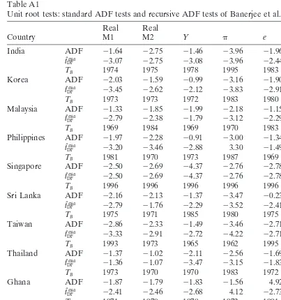
However, a number of authors (i.e., Perron, 1989) have pointed out that the standard ADF test is not appropriate for the variables that may have undergone structural changes. To examine the stationarity of variables with a structural break, we use the recursive version of the Banerjee et al. (1992) test. The latter test is based on asymp-totic-distribution theory, which treats break dates as unknown a priori. The results are given in the Appendix Table A1.5
404 A.C. Arize et al. / International Review of Economics and Finance 8 (1999) 399–420
that the null hypothesis of a unit root (i.e., nonstationarity) is accepted for the vari-ables, some caution is necessary. It is thus assumed that these series are integrated of order one.
3.2. Structural break
Given that we have I(1) variables, an Ordinary Least Squares (OLS) equation linking some of these variables will not be a mere spurious regression only if theI(1) variables are cointegrated. A possible reason for the failure to find cointegration using the Engle and Yoo (1987) methodology6may be due to structural instability in the
long-run relationship given in Eq. (1), especially since their test for linear cointegration presumes that the parameters of the equation are time-invariant and is therefore inappropriate during a period undergoing institutional changes. Gregory and Hansen (1996) propose extensions of the ADF test that allow for a regime shift in either the intercept or the entire coefficient vector. As Gregory and Hansen (1996, p. 101) noted, their residual-based tests “are useful in helping lead an applied researcher to a correct model specification.” A major advantage of this procedure is that it allows one to search for a break at an unknown shift point and to test for cointegration. Here, we imposed a priori, as well as estimated endogenously the breakpoints.7
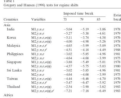
The results of applying the Gregory and Hansen (1996) method are summarized in Table 1. It presents the test statistics for cointegration at the estimated breakpoints and, for comparison, the test statistics achieved for pre-selected breakpoints. The timing of the structural break is shown in years and expressed in proportion to the sample sizes.
Three key points are highlighted by the results. First, the endogenously estimated break dates vary across countries and real balances. Second, for most of the countries (i.e., 9 out of 12) the results show that the variables bear a stationary relationship after accounting for a structural break. This finding suggests that there is a long-run equilibrium relationship among either real M1 or real M2, real income, inflation and openness variables in at least nine out of 12 countries. The null hypothesis of no cointegration with structural change is not rejected in Morocco, South Africa and the Philippines. However, the absolute values of the calculated Gregory and Hansen (1996) test statistic for the three countries are close to the 10% critical values, although not significant. The lack of cointegration may simply be the product of the low power of the test for samples below 50 (Gregory & Hansen, 1996, p. 110) when the autocorrelation coefficient is close to one. Finally, in general, the pre-selected breakpoints are not statistically significant.
3.3. Multivariate cointegration
A.C. Arize et al. / International Review of Economics and Finance 8 (1999) 399–420 405 Table 1
Gregory and Hansen (1996) tests for regime shifts
Estimated Imposed time break Estimated breakpoint
Countries Variables 73 79 85 breakpoint test statistic
Asia
India M1,y,p,e 25.04 25.19 23.86 1978 [0.52] 27.22
M2,y,p,e 25.27 25.38 24.61 1979 [0.48] 25.38 Korea M1,y,p,e,s(φ) 25.11 23.74 24.58 1976 [0.38] 27.72 M2,y,p,e,s(φ) 24.00 24.98 25.26 1978 [0.44] 25.42 Malaysia M1,y,p,e,rf 24.65 25.99 25.09 1974 [0.36] 26.31 M2,y,p,e,rf 24.51 24.18 24.49 1988 [0.79] 25.24 Philippines M1,y,p,e 23.02 25.85 24.96 1981 [0.54] 26.24 M2,y,p,e 24.64 24.68 23.99 1975 [0.37] 25.24 Singapore M1,y,p,e,s(φ) 23.88 25.49 25.01 1978 [0.42] 26.01 M2,y,p,e,s(φ) 24.57 25.75 25.03 1980 [0.48] 26.37 Sri Lanka M1,y,p,e 23.02 25.85 24.96 1981 [0.56] 26.25 M2,y,p,e 24.64 24.68 23.99 1975 [0.38] 25.24 Taiwan M1,y,p,e,s(φ) 24.44 26.46 24.70 1976 [0.50] 26.73 M2,y,p,e,rf 25.47 26.47 25.92 1979 [0.51] 26.47 Thailand M1,y,p,e,s(φ) 22.54 23.90 23.62 1983 [0.61] 24.26 M2,y,p,e,s(φ),rf 27.21 27.18 26.49 1983 [0.61] 28.41 Africa
Ghana M1,y,p,e,rf 24.55 25.17 24.28 1980 [0.56] 25.33 M2,y,p,e,rf 24.43 25.20 24.47 1980 [0.56] 25.32 Morocco M1,y,p,e,rf 24.55 24.67 24.96 1976 [0.41] 26.01 M2,y,p,e 22.49 22.80 24.28 1985 [0.68] 24.28 S. Africa M1,y,p,e,s(φ) 23.88 25.49 25.01 1978 [0.42] 26.01 M2,y,p,e,s(φ),rf 24.51 24.18 24.49 1988 [0.73] 25.24 Tunisia M1,y,p,e 23.38 25.85 24.97 1981 [0.54] 26.25 M2,y,p,s(φ) 24.16 25.30 24.73 1979 [0.45] 25.30 The critical values at the 10% level are25.75 form53 (i.e., for India,mis 3 and for Singapore,m
is 4 and26.17 form54. The critical values are from Table 1 of Gregory and Hansen (1996). There are no critical values form > 5. The imposed time breaks represent oil price shocks and the Plaza Accord of 1985.
(Johansen, 1995), and it is robust to departures from normality (Cheung & Lai, 1993; Johansen, 1995) and heteroskedasticity (MacDonald & Taylor, 1991; Johansen, 1995). Furthermore, Johansen (1995) points out that the power of the Johansen test is better than that of the residual-based tests. The test utilizes two likelihood-ratio (LR) test statistics for the number of cointegrating vectors: namely, the trace and the maximum eigenvalue (l-max) statistics. To perform the test, the conditioning vector includes the step and impulse or spike dummy variables (where applicable).8Similar dummies
are included in the studies by Hoffman et al. (1995, p. 322) and Hendry and Doornik (1994, pp. 11–13).
406 A.C. Arize et al. / International Review of Economics and Finance 8 (1999) 399–420
serial correlation.9After deciding the lag length in the VAR, we then followed the
procedure in Johansen (1995) to test the joint hypothesis of both the rank order and the deterministic components. The presence of a significant cointegration vector or vectors indicates a stable relationship among the relevant variables.
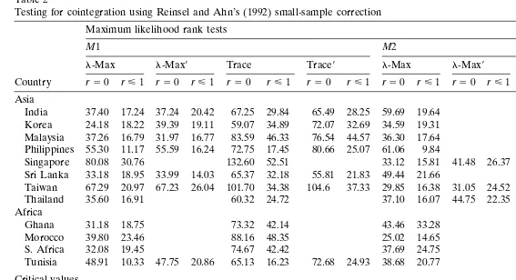
Table 2 reports the estimated thel-max and trace test statistics and their attendant critical values. These estimated test statistics have been adjusted by Reinsel and Ahn scaling factor discussed in Cheung and Lai (1993). For space reasons, we report only tests for the null hypothesesr50 andr<1. To facilitate an appropriate interpretation of our results, we also report the results with and without shift or step dummies.10
Focusing on the l-max test results, the null hypothesis tested is that there is no cointegrating vector,r50 and the null hypothesis of at most one cointegrating vector (Ho:r<1) is not rejected in any country (except the real M1 and real M2 results for
Singapore and Ghana, respectively).11
In each of the 12 cases, we can reject the hypothesis of no cointegration. Thus, a stable demand for real money balances (real M1 and real M2) exists during the period for each country.12 We also tested for evidence of cointegration among real money
balances, real income and expected inflation, and the results (not reported here) show that there is no evidence of cointegration in both real M1 and real M2 equations of Korea, Malaysia, Morocco and Tunisia. These results suggest that the openness vari-ables are important in the MDF of these countries in order for cointegration to be achieved.
3.4. Long-run equilibrium estimates
Given the relatively small sample available and the presence of one cointegrating relationship in the results of each country, we estimate and test the coefficients of Eq. (1) using two alternative approaches, the dynamic ordinary least squares (DOLS) estimator of Stock and Watson (1993) and the fully modified ordinary least-squares (FM-OLS) estimator of Phillips and Hansen (1990).13The former allowed the inclusion
of the dummies mentioned earlier, whereas the latter procedure does not allow these dummies. Examining the results reported in Table 3 enables us to determine to what degree these estimates are affected by the inclusion of dummies.
Focusing on the results obtained from the FM-OLS estimator, the hypothesis that MDF is homogenous of degree one with respect to the price level is tested first with only the traditional variables and second with both the traditional and openness variables. These results are reported in Table 3. With only the traditional variables (i.e., without openness variables) this hypothesis is rejected in 12 (i.e., five cases for real M1 and seven cases for real M2) out of 24 cases. With both the traditional and openness variables included, the hypothesis is rejected in only seven (i.e., four cases for real M1 and three cases for real M2) out of 24 cases. This latter finding showing that only seven are rejected and the cointegration results discussed above lend credence to the importance of the openness variables in the MDF of LDCs.
→
A.C.
Arize
et
al.
/
International
Review
of
Economics
and
Finance
8
(1999)
399–420
407
Table 2
Testing for cointegration using Reinsel and Ahn’s (1992) small-sample correction
Maximum likelihood rank tests
M1 M2
l-Max l-Max9 Trace Trace9 l-Max l-Max9 Trace Trace9
Country r50 r<1 r50 r<1 r50 r<1 r50 r<1 r50 r<1 r50 r<1 r50 r<1 r50 r<1
Asia
India 37.40 17.24 37.24 20.42 67.25 29.84 65.49 28.25 59.69 19.64 85.68 25.99 Korea 24.18 18.22 39.39 19.11 59.07 34.89 72.07 32.69 34.59 19.31 71.52 36.95 Malaysia 37.26 16.79 31.97 16.77 83.59 46.33 76.54 44.57 36.30 17.64 78.71 42.41 Philippines 55.30 11.17 55.59 16.24 72.75 17.45 80.66 25.07 61.06 9.84 75.92 14.86
Singapore 80.08 30.76 132.60 52.51 33.12 15.81 41.48 26.37 68.29 35.17 87.97 46.49 Sri Lanka 33.18 18.95 33.99 14.03 65.37 32.18 55.81 21.83 49.44 21.66 88.54 39.10
Taiwan 67.29 20.97 67.23 26.04 101.70 34.38 104.6 37.33 29.85 16.38 31.05 24.52 62.73 32.88 74.68 43.63 Thailand 35.60 16.91 60.32 24.72 37.10 16.07 44.75 22.35 81.87 44.77 103.39 58.64 Africa
Ghana 31.18 18.75 73.32 42.14 43.46 33.28 110.4 66.93
Morocco 39.80 23.46 88.16 48.35 25.02 14.65 48.45 23.43
S. Africa 32.08 19.45 74.67 42.42 37.69 24.75 95.12 57.42
Tunisia 48.91 10.33 47.75 20.86 65.13 16.23 72.68 24.93 38.68 20.77 64.30 25.62
Critical values
95% 27.42 21.12 48.88 31.54a
90% 24.99 19.02 45.70 28.78
95% 33.64 27.42 70.49 48.88b
90% 31.02 24.99 66.23 45.70
95% 39.83 33.64 95.87 70.49c
90% 36.84 31.02 91.40 66.23
The test statistics are adjusted for degrees of freedom following Reinsel and Ahn (1992) and the critical values are taken from Pesaran and Pesaran (1997) (unrestricted intercepts and no trends in VAR model).l-Max9and Trace9show test statistics when step dummines are included.
→
Arize
et
al.
/
International
Review
of
Economics
and
Finance
8
(1999)
399–420
Phillips and Hansen (1990) estimates elasticity Stock and Watson estimates elasticity
Traditional With Without Traditional With Without
variables Openness variables openness openness variables Openness variables openness openness
variables variables variables variables
Country y p e s(φ) rf y p e s(φ) rf
Asia
India M1 0.83 20.01 0.01 0.99 1.02 0.99 20.01 0.02 1.03 1.31
[17.26] [2.01] [3.06] [0.07] [0.18] [11.09] [2.60] [3.28] [1.03] [1.36]
M2 1.77 20.01 20.01 1.15 1.13 1.79 20.01 20.01 0.94 1.30
[35.07] [2.52] [3.59] [1.20] [1.04] [32.75] [1.96] [4.23] [0.52] [1.82]*
Korea M1 0.95 20.01 20.01 20.20 1.06 0.90 0.92 20.01 20.01 20.24 1.12 0.86
[44.87] [0.95] [6.10] [13.97] [0.65] [0.50] [19.71] [2.70] [2.11] [10.24] [0.73] [0.99]
M2 0.96 0.01 0.01 20.36 2.02 1.44 0.74 0.01 0.01 20.52 1.39 1.36
[12.43] [0.04] [1.30] [6.78] [5.70]* [1.19] [10.29] [1.05] [2.53] [8.67] [1.76]* [0.95]
Malaysia M1 1.25 0.01 0.14 20.02 1.26 1.54 1.19 0.02 0.17 20.02 1.30 1.21
[49.14] [2.76] [1.91] [3.78] [1.32] [1.64] [20.50] [3.30] [1.54] [2.07] [0.96] [0.38]
M2 1.54 20.02 20.28 20.01 1.21 1.74 1.62 20.02 20.15 20.01 1.16 1.18
[81.92] [5.17] [5.24] [3.59] [1.09] [3.78]* [61.90] [4.04] [2.94] [3.62] [0.39] [0.82]
Philippines M1 0.58 20.01 0.01 0.90 1.04 0.63 20.01 0.02 0.92 0.95
[5.65] [2.53] [1.60] [0.83] [0.88] [15.19] [2.62] [3.29] [0.70] [0.76]
M2 0.89 20.01 0.03 1.32 1.37 1.39 20.03 0.01 1.04 1.21
[5.60] [3.38] [5.61] [1.66] [5.44]* [5.45] [5.75] [2.74] [0.22] [2.62]*
Singapore M1 0.73 20.01 20.21 0.02 1.08 1.06 0.74 20.01 20.21 0.02 1.20 1.16
[32.05] [7.40] [6.32] [2.82] [1.11] [0.85] [22.36] [1.96] [4.71] [1.73] [3.73]* [2.34]*
M2 1.36 20.01 0.26 20.06 0.88 0.84 1.29 20.01 0.18 20.02 0.83 0.63
[16.88] [1.74] [2.20] [2.56] [0.90] [1.12] [20.40] [3.13] [2.08] [2.04] [1.14] [1.54]
Sri Lanka M1 0.58 20.01 0.01 0.75 1.14 0.56 20.01 0.01 0.48 1.11
[8.44] [0.99] [2.64] [1.40] [2.14]* [8.96] [2.58] [2.32] [3.41]* [1.48]
M2 0.97 0.01 0.01 0.02 1.10 0.70 0.01 0.01 0.69 1.07
[9.24] [0.57] [1.74] [3.67]* [1.09] [5.39] [1.14] [1.89] [1.19] [0.55]
Taiwan M1 1.50 20.01 20.01 0.05 1.16 0.95 1.43 20.03 20.01 0.06 0.96 0.67
[83.43] [5.13] [3.25] [2.46] [1.53] [0.40] [50.69] [10.56] [5.63] [3.83] [0.18] [2.03]*
→
A.C.
Arize
et
al.
/
International
Review
of
Economics
and
Finance
8
(1999)
399–420
409
Table3 (Continued)
Tests Tests
Zero price level Zero price level
Phillips and Hansen (1990) estimates elasticity Stock and Watson estimates elasticity
Traditional With Without Traditional With Without
variables Openness variables openness openness variables Openness variables openness openness
variables variables variables variables
Country y p e s(φ) rf y p e s(φ) rf
Asia
Taiwan M2 1.56 20.01 20.03 20.01 1.02 0.62 1.58 20.01 20.02 20.02 0.99 0.49
[56.89] [4.02] [7.47] [2.05] [0.34] [2.87]* [76.85] [9.34] [4.88] [3.94] [0.22] [3.00]*
Thailand M1 0.81 20.01 20.03 20.02 0.62 0.64 0.75 20.01 20.04 20.03 0.73 0.67
[24.40] [2.04] [3.31] [1.42] [7.51]* [4.98]* [27.42] [2.38] [2.27] [3.18] [2.49]* [7.41]*
M2 1.49 20.01 0.04 0.02 20.01 1.05 1.22 1.56 20.01 0.09 0.04 20.03 0.97 1.10
[83.42] [2.51] [8.37] [2.45] [1.48] [0.90] [2.93]* [326.5] [12.79] [46.9] [53.60] [30.15] [1.35] [1.10] Africa
Ghana M1 1.17 20.01 20.01 20.02 0.98 0.95 1.12 20.01 20.01 20.02 1.08 0.95
[15.30] [2.21] [10.8] [3.70] [0.95] [6.02]* [10.79] [0.41] [4.13] [2.22] [1.65] [4.77]*
M2 1.40 20.01 20.01 20.01 0.97 0.96 1.77 0.01 20.01 20.02 1.00 0.95
[17.64] [1.70] [8.84] [1.78] [1.35] [5.77]* [12.06] [1.18] [3.10] [2.25] [0.23] [6.79]*
Morocco M1 1.37 0.04 20.02 20.02 1.51 1.06 1.34 20.01 20.04 20.02 1.49 0.60
[21.59] [0.95] [1.88] [3.55] [6.36]* [0.50] [17.79] [0.18] [3.72] [3.34] [4.96]* [1.55]
M2 1.38 20.01 0.02 1.58 1.33 1.52 20.01 20.02 1.21 1.16
[24.41] [1.24] [1.85] [9.31]* [3.72]* [39.88] [2.77] [1.77] [1.88]* [1.48]
S. Africa M1 0.88 20.03 0.13 0.08 1.43 1.17 0.59 20.04 0.15 0.19 0.99 1.19
[6.65] [3.59] [5.13] [1.77] [4.82]* [4.48]* [4.27] [6.13] [5.97] [5.29] [0.05] [3.56]*
M2 1.54 20.02 0.06 20.09 20.02 0.91 1.11 1.70 20.01 20.05 20.11 20.03 1.02 1.11
[9.68] [2.14] [1.91] [2.29] [2.12] [0.96] [2.84]* [8.21] [3.51] [1.76] [1.82] [3.59] [0.16] [1.72]*
Tunisia M1 0.99 0.01 20.32 0.47 0.58 0.84 0.01 20.58 0.78 0.57
[18.17] [0.14] [2.09] [2.26]* [3.59]* [16.83] [3.47] [2.11] [0.93] [1.58]
M2 1.27 20.01 20.04 0.99 1.02 1.25 20.01 20.03 1.00 1.04
[58.56] [0.72] [1.90] [0.08] [0.24] [45.15] [2.27] [2.32] [0.03] [2.28]*
The numbers in brackets below the individual coefficient estimates are the absolute values oft-statistics. For testing price homogeneity, we report the estimated coefficient on the price level variable, in addition, to thet-statistic to test whether this coefficient is different from 1.
410 A.C. Arize et al. / International Review of Economics and Finance 8 (1999) 399–420
increase in the price level and money balances leads to a different level of real money balances. Assuming that M2 is chosen as the monetary target by the monetary authorities in Korea, our results imply that a 1% increase in the price level leads to a 2.02% increase in the demand for nominal M1. A possible explanation for this may be that, as the price level, increases the real cost of transactions experienced by economic agents also rises. This is different from the results reported for nominal balances in the United States. For instance, Arize and Darrat (1994) reported a price elasticity of less than one for the U.S. economy. Our results for Korea’s M2 suggest that to control inflation under 10%, the growth rate of M2 should be 29.8%, assuming the economy grows at 10% per year.14 Finally, as Hafer and Kutan (1994) noted, if
the demand for money is a demand for real balances, a price elasticity inconsistent with unity should cast doubt on whether the reported relationship is indeed a function of the money demand.
The long-run real income elasticities are also reported in Table 3 for real M1 and real M2, respectively. For the FM-OLS, the long-run elasticity of money demand with respect to real GDP has the expected positive signs in all countries. They range from 0.58 (Sri Lanka) to 1.50 (Taiwan) for real M1 and 0.89 (Sri Lanka) to 1.77 (India) for real M2. For the DOLS method, real income is positive and significant in all cases and ranges from 0.56 to 1.43 for real M1, whereas for real M2, the range is from 0.70 to 1.96. This implies a fairly large response of real money balances to changes in real income. A test of whether long-run real income elasticities of the demand for real money balances is unity indicates that this hypothesis is rejected in most of the countries, a verdict that is corroborated by the work of Aghevli et al. (1979). This finding implies that, as income rises, velocity tends to decline. Although there are exceptions, it can be argued that there is absence of economies of scale in money holdings in LDCs.
The sign, magnitude and significance of the long-run elasticity of money demand with respect to inflation is consistent with previous studies (i.e., Zilberfarb, 1988) and range from20.01 to20.03 for real M1 and20.01 to20.02 for real M2. For real M1, we do not believe that the positive sign in the case of Malaysia is credible. For the DOLS method, the range is20.01 to20.04 for real M1; however, significantly positive coefficients are obtained for Malaysia and Tunisia. For real M2, the inflation coeffi-cients in India, Korea, Sri Lanka, Ghana and Thailand are negative but nonsignificant. An appealing aspect of the results is that exchange rate is statistically significant in all countries (except Tunisia’s broad MDF). For real M1, it has a negative sign in seven countries and ranges from20.01 to20.21, whereas the sign is positive in India, Malaysia, the Philippines, Sri Lanka and South Africa (0.01 to 0.14). For real M2, it has a negative sign in four countries (20.01 to 20.28) and a positive sign in six countries (0.01 to 0.26). The DOLS estimates are similar to those of the FM-OLS method. It is worth mentioning that the effect of exchange rate on real money balances is largely positive (i.e., consistent with the Arango and Nadiri (1981) hypothesis) when it is the broad MDF and negative when it is the narrow MDF.15
A.C. Arize et al. / International Review of Economics and Finance 8 (1999) 399–420 411 Table 4
Speed of adjustments and mean time lags for adjustments of real balances [estimates from Phillips and Hansen (1990) procedure]
Mean time lags for adjustments of real balances* Speed of
adjustments M1 M2
Country M1 M2 y p e s(φ) rf y p e s(φ) rf
Asia
India 20.47 20.27 0.01 1.90 1.87 0.81 1.19 1.24
Korea 20.73 20.19 0.21 1.47 1.46 1.50 0.70 1.83 1.81 1.99
Malaysia 20.69 20.41 0.23 0.80 0.95 0.78 1.77 1.86 2.50 1.84
Philippines 20.49 20.31 0.39 2.16 2.23 1.96 2.06 2.14 Singapore 20.73 20.29 0.06 1.36 1.26 1.35 0.14 2.39 2.70 2.36
Sri Lanka 20.65 20.36 1.38 0.54 0.52 1.13 1.07 1.02
Taiwan 20.61 20.56 1.28 0.95 0.97 0.92 1.33 1.54 1.56 1.57
Thailand 20.37 20.73 0.01 1.84 1.96 1.82 0.22 1.26 1.25 1.26 1.28 Africa
Ghana 20.66 20.59 1.20 1.25 1.25 1.24 0.91 1.27 1.27 1.26
Morocco 20.41 20.29 2.42 2.34 2.48 2.38 2.70 2.61 2.66
South Africa 20.54 20.54 0.52 2.01 1.91 1.76 0.79 1.19 1.52 0.78 1.15
Tunisia 20.35 20.43 0.01 2.47 1.11 0.59 1.31 1.31
* Absolute values.
on the risk measure is20.20 for Korea and20.02 for Thailand. These results support the Akhtar and Putnam (1980) hypothesis, whereas the estimates for Singapore (0.02) and Taiwan (0.05) are consistent with the Zilberfarb (1988) hypothesis of a positive effect of exchange-rate risk on real money balances. For real M2, the foreign exchange risk variable is statistically significant in five countries. The estimated coefficients are
20.36, 20.06, 0.02, 20.09 and 20.04 for Korea, Singapore, Thailand, South Africa and Tunisia, respectively. These results are similar to those obtained using the DOLS estimates.
For the FM-OLS method, the foreign interest rate variable is significantly negative, and the semi-elasticity is about20.02 in the long-run real M1 equations for Malaysia, Ghana and Morocco. For the real M2 equations, the long-run semi-elasticity is about
20.01 in Malaysia, Taiwan, Thailand and Ghana, and 20.02 in South Africa. These results are consistent with those reported for the DOLS estimator.
3.5. Speed of adjustment and mean time lags
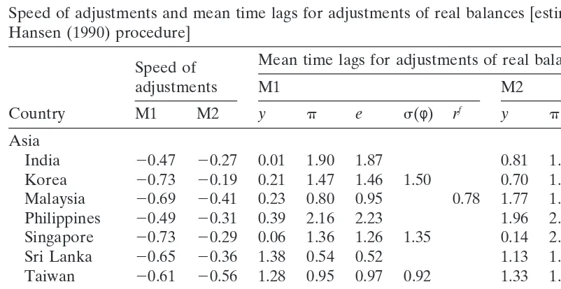
This section provides information on the speed of adjustment to equilibrium and identifies how quickly real balances respond to changes in the determinants. Table 4 reports the coefficient of the error-correction term and the mean time lag of each explanatory variable.16These results were obtained by estimating Eq. (2) for each of
the 12 countries.17
412 A.C. Arize et al. / International Review of Economics and Finance 8 (1999) 399–420
For both real M1 and real M2, there is considerable inter-country variation in the adjustment speed to the last period’s disequilibrium. In the case of real M1, the coefficient of the error-correction term ranges from a low of 0.35 for Tunisia to a high of 0.73 for Korea, whereas for real M2, the range from a low of 0.29 for Singapore and Morocco to a high of 0.73 for Thailand. For example, in Singapore and Morocco, only about 29% of adjustment occurs in a year, whereas the figure is 73% for Thailand. Our results imply that the adjustment of real money balances to changes in the regressors may take about three years in Singapore and Morocco to a little below one and a half years in Thailand. This indicates the existence of market forces in the monetary sector that operate to restore long-run equilibrium after a short disturbance. Three points are worthy of mention. First, our results are not consistent with the hypothesis of an instantaneous adjustment of the rate of growth of real money balances to departure from their equilibrium value in the previous period. Second, our rela-tively large speeds of adjustment suggest that the predictive content of the relation-ship between real balances and their determinants have not deteriorated over time. Finally, because M2 contains a savings component, the speed of adjustment is below that of M1.18
The mean time shows that the average time lag for adjustment of real money balances to changes in each independent variable. The results suggest that the mean lag for adjustment of real money balances to changes in real income is approximately one year in almost all cases. In the case of inflation, it takes about two years in the majority of the countries when the model is real M1, except for Malaysia, Sri Lanka and Taiwan, where it is about a year. For real M2, it takes more than one year in all countries and close to three years in Morocco.
Given the open nature of LDCs, another interesting aspect of our study is that the average time lag for the adjustment of real money balances to changes in the openness variables is fairly short.19 For the majority of the countries, the mean time lags for
exchange rate, foreign exchange risk and foreign interest rate are below two years for both real M1 and M2.20In sum, the response of real money balances to changes
in real income is similar to the response to changes in the “openness” variables.
3.6. Choice of a monetary aggregate
A.C. Arize et al. / International Review of Economics and Finance 8 (1999) 399–420 413
M1 or M2 can be used to achieve the objective of price stability. Our findings also support the conclusion by Chowdhury (1997, p. 407) that the appropriate MDF for Thailand is real M2. Like Bahmani-Oskooee and Rhee (1994), our results point to real M1 as the appropriate MDF for Korea.
Concerning the short-run dynamics, the results favor both M1 and M2. First, we employed Sargan’s likelihood criterion recommended in Pesaran and Pesaran (1997, pp. 364–367). The results of this measure favor both M1 and M2. For example, Sargan’s criterion chose M2 for Malaysia, the Philippines, Sri Lanka, Thailand, Singapore and Morocco, whereas for India, Korea, Taiwan, Ghana, South Africa and Tunisia, it chose M1.
Second, following the procedure outlined in Baye and Jensen (1995, pp. 645–647), we found that the estimated slope coefficient of a three-year moving average of M2 growth is positive and larger in size than those obtained using M1 growth in six out of 12 countries (i.e., India, South Africa, Tunisia, Morocco, Taiwan and Ghana), whereas in the other six countries, this procedure favored M1. These results imply that if the objective of the monetary authorities is the achievement of greater price stability, then either M1 or M2 can be used as a monetary target.
4. Conclusions
This article has presented the first conclusive evidence on the long-run equilibrium relationship among the following variables: the real balance of M1 or M2, real income, inflation, exchange rate, foreign exchange risk and foreign interest rates in LDCs. As far we know, there is no such study in the literature for a diverse sample of developing countries.
Because the unit root properties of the data play a key role in the analysis, we used two sets of statistics that examine the unit root hypothesis without allowing for trend breaks: (1) ADF t-statistics and (2) 95% confidence intervals for the largest autoregressive root. We then employed the recursive minimum ADF test recom-mended in Banerjee et al. (1992), which treats break dates as unknown a priori. The results from these tests provide evidence in favor of a single unit root in all variables. Therefore, treatment of this nonstationarity is essential for meaningful results.
After testing for cointegration using the Engle and Yoo (1987) approach, we applied the Gregory and Hansen (1996) pre-test procedure to search for a structural break in the long-run relationship between the real balance of M1 or M2 and its determinants. Where concern was warranted, the results from Johansen’s multivariate procedure were obtained by treating the dummy variable (representing the structural break revealed by the Gregory and Hansen (1996) method), as a weakly exogenous variable. The empirical results suggest that the demand for money balances and its economic arguments not only are cointegrated but also tie closely together in their short-run dynamics.
414 A.C. Arize et al. / International Review of Economics and Finance 8 (1999) 399–420
they imply that monetary authorities can use monetary policy successfully, both in the conduct of stabilization policy as well as in their efforts to mobilize the necessary capital for non-inflationary investment spending. In addition, the results also suggest that monetary policy actions aimed at stabilizing the domestic economy can generate at best only uncertain results if the effects of the openness variables (i.e., exchange rate) are ignored in the execution of monetary policy.
Acknowledgments
The authors would like to thank Ed Manton, Keith McFarland and Lee Schmidt for helpful comments on an earlier draft. Special thanks to Kathleen Smith for excellent research assistance. We are grateful to Craig Hakkio for his valuable suggestions in calculating the median lags. This research is funded by a GSRF-TAMU-C grant.
Notes
1. See Domowitz and Hakkio (1990, p. 30) for a detailed explanation of the importance of deflating by consumer price index and using real GDP as scale measure.
2. The consequences of nonstationarity is the inapplicability of the standard sam-pling theory. The cointegration approach is attractive in that it can properly account for the nonstationary series.
3. Some observations were lost due to the construction of the real exchange-rate risk and the inflation variables, so the effective estimation period is 1961 through 1996. It is worth mentioning that the inclusion of exchange rate, foreign interest rate and real exchange-rate risk in the model also handles the problem of estimating over two exchange-rate periods. Nonetheless, the data may contain several structural breaks. Later, we will test if the data show any structural breaks in the long-run money demand function of these countries.
4. This proxy is constructed by the moving-sample standard deviation expressed as
s(φ)t1m 5[m1
o
mi51
(Rt1i212Rt1i22)2]1/2
A.C. Arize et al. / International Review of Economics and Finance 8 (1999) 399–420 415 Table A1
Unit root tests: standard ADF tests and recursive ADF tests of Banerjee et al. (1992)
Real Real
Country M1 M2 Y p e s(φ) rf
India ADF 21.64 22.75 21.46 23.96 21.96 24.01 21.76
tˆmin
DF 23.07 22.75 23.08 23.96 22.44 24.01 24.18
TB 1974 1975 1978 1995 1983 1985 1979
Korea ADF 22.03 21.59 20.99 23.16 21.90 23.51 21.76
tˆmin
DF 23.45 22.62 22.12 23.83 22.91 23.59 24.18
TB 1973 1973 1972 1983 1980 1995 1979
Malaysia ADF 21.33 21.85 21.99 22.18 21.15 22.28 21.56
tˆmin
DF 22.79 22.38 21.79 23.12 22.29 24.74 24.18
TB 1969 1984 1969 1970 1983 1976 1979
Philippines ADF 21.97 22.28 20.91 23.00 21.34 24.11 21.56
tˆmin
DF 23.20 23.46 22.88 3.30 21.49 24.11 24.18
TB 1981 1970 1973 1987 1969 1993 1979
Singapore ADF 22.50 22.69 24.37 22.76 22.78 2.27 21.76
tˆmin
DF 22.50 22.69 24.37 22.76 22.78 24.41 24.18
TB 1996 1996 1996 1996 1996 1972 1979
Sri Lanka ADF 22.16 22.13 21.37 23.47 20.23 22.73 21.56
tˆmin
DF 22.79 21.76 22.29 23.52 22.41 23.51 24.18
TB 1975 1971 1985 1980 1975 1972 1979
Taiwan ADF 22.86 22.33 21.49 23.46 22.71 22.87 21.76
tˆmin
DF 23.33 22.91 22.72 24.22 22.71 22.87 24.18
TB 1993 1973 1965 1962 1995 1995 1979
Thailand ADF 21.37 21.02 22.11 22.56 21.69 22.63 21.76
tˆmin
DF 21.36 21.07 23.47 23.15 21.83 23.00 24.18
TB 1973 1970 1970 1983 1972 1990 1979
Ghana ADF 21.87 21.79 21.83 21.56 4.92 21.67 21.56
tˆmin
DF 22.41 22.46 22.68 4.12 22.73 23.49 24.18
TB 1971 1970 1978 1973 1991 1987 1979
Morocco ADF 22.57 22.77 21.18 21.55 21.91 21.47 21.56
tˆmin
DF 23.26 23.36 23.09 22.12 22.24 23.58 24.18
TB 1977 1978 1979 1973 1986 1986 1979
S. Africa ADF 22.79 22.42 21.17 20.06 0.84 21.48 21.56
tˆmin
DF 22.49 22.42 23.05 21.13 0.63 22.86 24.18
TB 1969 1996 1980 1971 1976 1979 1979
Tunisia ADF 20.62 20.93 21.47 23.62 21.53 23.97 21.56
tˆmin
DF 23.56 23.60 22.83 23.79 22.61 23.97 24.18
TB 1970 1971 1971 1985 1986 1993 1979
TBis the estimated break date. The critical values are23.45 (approx.) for ADF and24.33 for tˆDFmin at the 5% significant level.
416 A.C. Arize et al. / International Review of Economics and Finance 8 (1999) 399–420
Table A2
Description and sources of data
Mean of Mean of
Country Sample period Observations inflation exchange rate
Asia
India 1962–1994 33 8.32 11.28
Korea 1964–1995 32 12.66 563.68
Malaysia 1962–1994 33 3.58 2.66
Philippines 1962–1996 35 11.68 12.50
Singapore 1964–1996 33 3.59 2.31
Sri Lanka 1962–1995 34 8.61 19.39
Taiwan 1961–1995 35 5.15 36.19
Thailand 1964–1994 31 5.64 22.56
Africa
Ghana 1962–1993 32 33.07 81.75
Morocco 1962–1995 34 6.20 6.25
South Africa 1964–1996 33 10.30 1.56
Tunisia 1964–1996 33 6.10 0.64
Series and sources.International Financial Statistics(International Monetary Fund): money balances (M1), Line 34; quasi money, Line 35; broad money (M2), Line 34135; prices, Line 64; U.S. lending rate, Line 60b; real GDP, Line 99b.p or line 99b scaled by prices; official exchange rate, Line rf (domestic currency/U.S. dollar rate).
however, that some of the intervals are wide, suggesting a large amount of uncertainty. For example, the real M1 data in Thailand and South Africa are consistent with the hypothesis that the process is I(1), but also are consistent with the hypothesis that the data are trend stationary with autoregressive root close to 0.87. Because it is difficult to discriminate between trend stationarity and simple I(1) processes, we prefer to operate under the assumption of a stochastic trend in the series.
6. Some experimentations using the Engle and Yoo (1987) methodology and Bardsen (1989) approximate standard errors for testing the significance of the parameters of Eq. (1) indicate that we either fail at the 5% level or we find weak evidence of a stationary money demand function in most of the countries. Further, some of the “openness” variables proved statistically nonsignificant in some of the countries. For the rest of the article, we utilize our preferred equations for each country since our objective is to obtain a fairly parsimonious equation for each monetary aggregate.
7. Following Gregory and Hansen (1996), we compute ADF statistics for each breakpoint in the interval, 0.15Tto 0.85T(whereTis the number of observa-tions), and then we choose the breakpoint associated with the smallest value as that point at which the structural break occurred.
A.C. Arize et al. / International Review of Economics and Finance 8 (1999) 399–420 417
The step dummies (equivalent to a permanent intercept shift) were obtained from employing the Gregory and Hansen (1996) procedure. The impulse dummies were identified obtained from the inspection of the residuals according to the CUSUM/CUSUMQ method (not reported in this article).
9. The test statistic is 2(T2k/T) (likelihood [unrestricted]2likelihood[restricted]), and the maximum lag was set to two.
10. It is interesting to note that the cointegration test results actually are little affected by omitting the dummy variable. This suggests that even though the level of the empirical relationship may have shifted, the underlying economic relationship between real money balance and its determinants remained un-changed. Indeed, this explains why Clements and Mizon (1991) advocate the use of dummy variables instead of adding extra variables. See also Hafer and Kutan (1994).
11. The critical values recorded in Osterward-Lenum’s (1992) article are for a VAR without dummies. Because these were included outside the cointegration space in our empirical analysis, we used the adjusted critical values automatically sup-plied by the latest version of Microfity(4.0) statistical package. The authors are Pesaran and Pesaran (1997), and they note that “there are important differences between the critical values used in Microfit and those reported by Osterward-Lenum (1992).” Nevertheless, when dummies are include, we regard our results as indicative of cointegration; that is, they should be interpreted with caution. 12. We are grateful to a referee for reminding us about the problems associated
with employing small samples. Given unavailability of sufficient data for many LDCs, efforts were made to ensure that our data for each country meets the statistical definition of a large sample. The issue of finite sample bias is addressed by the use of Reinsel-Ahn corrected likelihood ratio test statistics in Table 2. However, note that Johansen (1995) and Doornik and Hendry (1994) point out that it is unclear yet whether this is the preferred correction. Also the limitation of our results with respect to the inclusion of a dummy variable is acknowledged. Readers should keep in mind this limitation when evaluating our work. Nevertheless, it is worth pointing out that with respect to real M2, the dummy variable is included only in three (Singapore, Taiwan and Thailand) out of 12 countries. Second, although the dummy variables are entered exoge-nously in this study, it is unclear that all the empirical issues involved with the inclusion of dummy variables in Johansen’s estimator can be eradicated by simulating finite-sample critical values that take into account breaks in the data [see a caveat in Cheung et al. (1995, p. 185)].
13. Stock and Watson (1993) found in their simulations that different estimators of the cointegrating estimators of the cointegrating vectors yield estimated coefficients that differ considerably in finite samples; hence, they suggest that researchers should not rely on one estimation technique. Monte Carlo results obtained by Stock and Watson (1993) show that the DOLS estimator has the lowest root-mean-square error and therefore performs well in finite samples relative to other asymptotically efficient estimators.
418 A.C. Arize et al. / International Review of Economics and Finance 8 (1999) 399–420
15. Using the mean of exchange rate and inflation reported in the Appendix Table A2, one can obtain the elasticities for inflation and exchange rate by multiplying their estimated coefficients by the mean of each variable. When this is done, in almost every case the elasticity with respect to exchange rate is larger than that of inflation. For example, for Taiwan’s real M2, the inflation elasticity is
20.052 (that is 20.01 3 5.15) and exchange rate elasticity is 21.086 (that is,
20.03336.19). The values 5.15 and 36.19 are the mean of inflation and exchange rate, respectively.
16. We perform a test of general parameter stability over the sample as a whole. The test involves forming a t-statistic for the mean of the recursive residuals, which has expectation zero under the null hypothesis of parameter stability (Madalla, 1988, pp. 414–415). The nth recursive residual is the scaled forecast error for the nth observation based on a regression involving the first n21 observations.
17. Although the Johansen procedure does provide estimates of the speed of adjust-ment of money holdings, it is useful to specify and estimate a second stage error correction model in order to subject the short-run dynamic model to tests (i.e., parameter stability and misspecification). Readers should keep in mind that no current terms were allowed in the short-run estimation and much of the above results supports a single cointegrating vector.
18. Cuthberston and Taylor (1990) have argued that the slow speed of adjustment is likely, especially if the precautionary saving motive of economic agents is significantly influenced by long-run considerations of future income and the rates of return. See also Feige’s (1967) observation that “if the major impact of financial innovation is to provide close substitutes for money, thus reducing the costs associated with the disequilibrium position, the effect may be to reduce the speed of cash balance adjustment.”
19. While the mean lag gives the mean (average) length of time to full adjustment, the median lag gives the time for 50% of the adjustment to occur. For real M1, the median lags with respect to exchange rate range from a low of 0.03 in Sri Lanka to 1.60 for Morocco; for foreign exchange risk, they range from 0.61 in Taiwan to 1.29 in Thailand; and for foreign interest rate, they range from 0.44 in Malaysia to a high of 1.56 for Morocco.
20. The median lags in the case of real M2 are also fairly short. For exchange rate, they range from a low of 0.72 in Sri Lanka to 1.69 in Singapore; for foreign exchange risk, they range from 0.81 in South Africa to 1.55 in Singapore; and for foreign interest rate, they range from 0.83 in South Africa to a high of 1.30 in Malaysia.
References
Adekunle, J. O. (1968). The demand for money: evidence from developed and less developed economies.
A.C. Arize et al. / International Review of Economics and Finance 8 (1999) 399–420 419 Aghevli, B. B., Khan, M. S., Narvekar S., & Short, B. K. (1979). Monetary policy in selected Asian
countries.International Monetary Fund Staff Papers 32, 775–784.
Akhtar, M., & Putnam, B. (1980). Money demand and foreign exchange risk: the German case.Journal of Finance 35, 787–794.
Arango, S., & Nadiri, I. M. (1981). Demand for money in open economies.Journal of Monetary Economics 7, 69–83.
Arize, A. C. (1989). An econometric investigation of money demand behavior in four Asian developing economies.International Economic Journal 3, 79–93.
Arize, A. C. (1994). A reexamination of the demand for money in small developing economies.Journal of Applied Economics 26, 217–227.
Arize, A. C., & Darrat, A. (1994). The value of time and recent U.S. money demand instability.Southern Economic Journal 60(3), 564–578.
Baba, Y., Hendry, D. F., & Starr, R. M. (1988). The demand for M1 in the U.S.A., 1960–1988.Review of Economic Studies 59, 25–61.
Bahmani-OsKooee, M., & Rhee, H.-J. (1994). Long-run elasticities of the demand for money in Korea: evidence from cointegration analysis.International Economic Journal 8, 1–11.
Bahmani-OsKooee, M., & Pourheydarin, M. (1990). Exchange rate sensitivity of the demand for money and effectiveness of fiscal and monetary policies.Applied Economics 22, 1377–1384.
Banerjee, A., Lumsdaine, R. L., & Stock, J. H. (1992). Recursive and sequential tests for a unit root: theory and international evidence.Journal of Business and Economic Statistics 10, 271–287. Bardsen, G. (1989). Estimation of a long-run coefficient in error-correction models.Oxford Bulletin of
Economics and Statistics 51, 345–350.
Baye, M. R., & Jensen, D. W. (1995).Money, Banking and Financial Markets: An Economics Approach.
New Jersey: Houghton Mifflin Company.
Branson, W. H., & Buiter, W. H. (1984). Monetary and Fiscal Policy with Flexible Exchange Rates in Economic Interdependence and Flexible Exchanges Rates, J. S. Bhandari & B. H. Putnam (Eds.). London: MIT Press.
Campbell, J. Y., & Perron, P. (1991). Pitfalls and Opportunities: What Macroeconomists Should Know about Unit Roots. In O. J. Blanchard & S. Fisher (Eds.), NBER (National Bureau of Economic Research) Macroeconomics Annual(pp. 144–201). Cambridge: MIT Press.
Cheung, Y.-W., Fung, Y.-W., Lai, K. S., & Lo, W.-C. (1995). Purchasing power parity under the European monetary system.Journal of International Money and Finance 14, 179–189.
Cheung, Y.-W., & Lai, K. S. (1993). Finite-sample sizes of Johansen’s likelihood ratio tests for cointegra-tion.Oxford Bulletin of Economics and Statistics 55, 313–328.
Chowdhury, A. R. (1997). The financial structure and the demand for money in Thailand. Applied Economics 29, 401–409.
Clements, M. P., & Mizon, G. E. (1991). Empirical analysis of macroeconomic time series: VAR and structural models.European Economic Review 35, 161–178.
Cuthberston, K., & Taylor, M. P. (1990). Money demand, expectations, and the forward-looking model.
Journal of Policy Modelling 12(2), 289–315.
Domowitz, I., & Hakkio, C. S. (1990). Interpreting an error correction model: partial adjustment, forward looking behavior, and dynamic, international money demand.Journal of Applied Econometrics 5, 29–46. Domowitz, I., & Elbadawi, I. (1987). An error-correction approach to money demand.Journal of
Develop-ment Economics 26, 257–275.
Doornik, J., & Hendry, D. F. (1994). PcFiml Version 8: Interactive Econometric Modelling of Dynamic Systems, Institute of Economics & Statistics, University of Oxford.
Engle, R, & Yoo, B. (1987). Forecasting and testing in cointegrated system.Journal of Applied Economet-rics 5, 143–159.
Feige, E. (1967). Expectations and adjustments in the monetary sector.American Economic Review 57, 467.
420 A.C. Arize et al. / International Review of Economics and Finance 8 (1999) 399–420
Gregory, A. W., & Hansen, B. E. (1996). Residual-based tests for cointegration in models with regime shifts.Journal of Econometrics 70, 99–126.
Hafer, R. W., & Kutan, A. M. (1994). Economic reforms and long-run money demand in China: implica-tions for monetary policy.Southern Economic Journal 60, 936–945.
Hakkio, C. S., & Rush, M. (1991). Cointegration: how short is the long run?Journal of International Money and Finance 10, 571–581.
Hamburger, M. J. (1977). The demand for money in an open economy.Journal of Monetary Economics 3, 25–40.
Hendry, D. D .F., & Doornik, J. A. (1994). Modelling linear dynamic econometric systems. Scottish Journal of Political Economy 45, 1–33.
Hoffman, D. L., Rasche, R. H., & Tieslau, M. A. (1995). The stability of long-run money demand in five industrial countries.Journal of Monetary Economics 35, 317–339.
Johansen, S. (1988). Statistical analysis of cointegrating vectors. Journal of Economic Dynamics and Control 12, 231–254.
Johansen, S. (1992). Determination of cointegration rank in the presence of a linear trend. Oxford Bulletin of Economics and Statistics 54, 383–397.
Johansen, S. (1995).Likelihood-Based Inference in Cointegrating Vector Autoregressive Models. New York: Oxford University Press.
Koray, F., & Lastrapes, W. D. (1989). Real exchange rate volatility and U.S. bilateral trade: a VAR approach.Review of Economics and Statistics 71, 708–712.
MacDonald, R., & Taylor, M. P. (1991). Exchange rates, policy convergence, and the European monetary system.Review of Economics & Statistics 73, 553–558.
Madalla, G. S. (1988).Introduction to Econometrics.New York: MacMillian Publishing Company. Marquez, J. (1987). Money demand in open economies: currency substitution model for Venezuela.
Journal of International Money and Finance 6, 167–178.
Mundell, A. R. (1963). Capital mobility and stabilization policy under fixed and flexible exchange rates.
Canadian Journal of Economics and Political Science 29, 475–485.
Ng, S., & Perron, P. (1995). Unit root tests in ARMA models with data-dependent methods for the selection of the truncation lag.Journal of the American Statistical Association 90, 268–281.
Osterwald-Lenum, M. (1992). A Note with quantiles of the asymptotic distributions of the maximum likelihood cointegration ranks test statistics: four cases.Oxford Bulletin of Economics and Statistics 54(3), 461–472.
Perron, P. (1989). The great crash, the oil price shock, and the unit root hypothesis.Econometrica 57, 1361–1401.
Pesaran, H. H., & Pesaran, B. (1997).Working with Microfit 4.0: interactive econometric analysis.England: Camfit Data Ltd.
Phillips, P. C. B. (1991). Optimal inference on cointegrating systems.Econometrica 59, 283–306. Phillips, P. C. B., & Hansen, B. E. (1990). Statistical inference in instrumental variables regression with
I(1) processes.The Review of Economic Studies 57, 99–125.
Stock, J. (1991). Confidence intervals for the largest autoregressive root in U.S. macroeconomic time series.Journal of Monetary Economics 28, 435–459.
Stock, J., & Watson, M. (1993). A simple estimator of cointegrating vectors in higher order integrated systems.Econometrica 61, 783–820.
Warner, D., & Kreinin, M. (1983). Determinants of international trade flows.Review of Economics and Statistics 65, 96–104.
Wickens, M. (1972). A note on the use of proxy variables.Econometrica 40(2), 759–761.