BOUNDARY DEPTH INFORMATION USING HOPFIELD NEURAL NETWORK
Sheng Xu, Ruisheng Wang*
Department of Geomatics, Engineering, University of Calgary, Calgary, Alberta, Canada T2N 1N4 - (sheng.xu2, ruiswang)@ucalgary.ca
Commission V, WG V/1
KEY WORDS: Boundary, Stereo Matching, Depth Information, Optimization, Discontinuity, Hopfield Neural Network
ABSTRACT:
Depth information is widely used for representation, reconstruction and modeling of 3D scene. Generally two kinds of methods can obtain the depth information. One is to use the distance cues from the depth camera, but the results heavily depend on the device, and the accuracy is degraded greatly when the distance from the object is increased. The other one uses the binocular cues from the matching to obtain the depth information. It is more and more mature and convenient to collect the depth information of different scenes by stereo matching methods. In the objective function, the data term is to ensure that the difference between the matched pixels is small, and the smoothness term is to smooth the neighbors with different disparities. Nonetheless, the smoothness term blurs the boundary depth information of the object which becomes the bottleneck of the stereo matching. This paper proposes a novel energy function for the boundary to keep the discontinuities and uses the Hopfield neural network to solve the optimization. We first extract the region of interest areas which are the boundary pixels in original images. Then, we develop the boundary energy function to calculate the matching cost. At last, we solve the optimization globally by the Hopfield neural network. The Middlebury stereo benchmark is used to test the proposed method, and results show that our boundary depth information is more accurate than other state-of-the-art methods and can be used to optimize the results of other stereo matching methods.
* Corresponding author
1. INTRODUCTION
Determination of correspondence between two pictures from different viewpoints of the same scene is the primary contribution of stereo matching. Various constraints have been used to find the optimal match, such as color consistency, gradient distribution, and geometric shape. Nevertheless, these constraints provide less information about discontinuities which is the bottleneck of stereo matching.
Compared with current matching methods, the proposed method is in our novel 3D space with less complexity, and has the constraint of discontinuities to find the optimal match. The main contributions of our work are in the following: 1) we obtain a new 3D space by radial basis information (RBI); 2) we form a new energy function to calculate the cost for the matching; 3) we convert the proposed objective function to a solvable Hopfield neural network (HNN) energy function.
2. RELATED WORK
Stereo matching methods can be divided into region-based and feature-based (Scharstein and Szeliski, 2002). Region-based algorithms use a sliding window to calculate the aggregation of the cost. Then various specific optimizations are followed to obtain the minimum cost for the matching, such as Graph Cut (Boykov et al., 2001) and Belief Propagation (Sun et al., 2003). Due to the propagation of errors in discontinuities, the accuracy of these methods is not satisfactory.
Feature-based algorithms pay attention to features and perform better in discontinuities. Shape based matching (Ogale and Aloimonos, 2005) has analyzed the effects of the shape of
established dense point correspondence to improve the matching, but the result in the repeated shape areas is imprecise. CrossTrees (Cheng et al., 2015) uses two priors: edge and super-pixel, which are proposed to avoid the false matching in discontinuities. However, the method fails to large planar surfaces with fewer features. Instead of using adjacent pixels for matching, LLR (Zhu et al., 2012) chooses neighborhood windows and believes there is a linear relationship between pixel values and disparities. However, it is sensitive to the size of the window and large areas devoid of any features. To eliminate improper connections on the boundaries of two objects, imprNLCA (Chen et al., 2013) uses the boundary cue of the reference image which is more reliable than the color cue in areas with similar colors. Nevertheless, imprNLCA shows less improvement in discontinuities compared to original NLCA (Yang, 2012). The Borders (Mattoccia et al., 2007) obtains the precise border localization based on a variable support method (Tombari et al., 2007) for retrieving depth discontinuities. However, for images with a large range of disparities, their accuracy decreases. LCVB-DEM (Martins et al., 2015) introduces a trained binocular neuronal population to learn how to decode disparities. With the help of monocular cells, they encode both line and edge information which are critical for persevering discontinuities. However, due to the fact that mechanism of cell responses is complex, their accuracy is far from what is desirable.
Algorithm (Nasrabadi and Choo, 1992) based on the variance equations for each direction is less robust with limited application. To enhance the robustness, methods (Lee et al., 1994) (Huang and Wang, 2000) (Achour and Mahiddine, 2002) (Laskowski et al., 2015) formulated their respective energy The International Archives of the Photogrammetry, Remote Sensing and Spatial Information Sciences, Volume XLI-B5, 2016
functions which contain the constraints of similarity, smoothness and uniqueness to work well on noisy images. Although the above Hopfield neural network (HNN) based matching methods choose different constraints and obtain a desirable result for regions of interests, they neglect the matching of discontinuities. Neurons in HNN are interconnected and therefore, the change of a neuron state will affect all other input neurons. HNN converges to a stable state by updating the neurons from the activation function. This implies that it can obtain the global optimization result automatically. Hence, we use the HNN model to solve our optimization problem.
Neurons in our method are based on the disparity space rather than the pixels in the left image and the right image as the aforementioned methods. For the formation of objective function, we use discontinuity information obtained from our novel 3D space to calculate matching cost, and constraints of uniqueness and position to reduce the search for a solution. To show the performance of our algorithm, we test it on Middlebury benchmark to present our accuracy and show the improvement of state-of-the-art methods by raising their accuracy in discontinuities.
3. THE METHOD
This section describes a new objective function for stereo matching, and shows the derivation of the proposed optimization method.
3.1 Energy Function
Stereo matching is about assigning the best disparity for each pixel. Figure 1 is the disparity space. Different methods relate to various cost paths from the first row to the last row. Result should be smooth on continuities and preserve discontinuities on disparity map. The key problems are the energy function and the optimization method.
… …
… …
… …
… …
… … …… …… ……
……
P1
P2
P3
Pn
0 1 2 3 dmax
cost path
Figure 1. Disparity space. There are n pixels, namely P1, P2, ...,
Pn, and their disparities are ranged from 0 to dmax. The cost path
relates to the assignment of disparities for each pixel.
The radial basis function gives an expression on the relationship between pixels and its neighbour (Buhmann, 2004). Thus, we calculate the surrounding information of a pixel P by
22 ' 2
) (
)
(
P P I
I
e
P
S
(1)In Eq.(1), IP is the intensity value of a pixel P, and σ is the
variance of neighbors of P. The neighbor pixels are selected by a window with a size of N. Figure 2(a) is the left image, and its surrounding information is shown from Figure 2(b) to 2(c) in
different N. A small N results sharp discontinuities and a large
N causes smooth discontinuities.
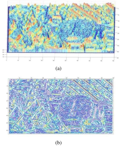
We describe a pixel P in a 3D space XYZ as (x, y, S) as shown in Figure 3(a) rather than only intensity. S is the surrounding information of the pixel at (x, y) in the image. The discontinuities are outstandingly visible and the continuities are smooth as shown in Figure 3(b). We call this space as RBI (Radial Basis Information) space and following is our objective function for the matching.
(a) (b)
(c) (d)
Figure 2. Surrounding information of Cones. (a) Original left image. (b) N=3. (c) N=5. (d) N=8.
(a)
(b)
Figure 3.Display of the RBI space. (a) Cones in the 3D RBI space. (b) The contour of Cones in the RBI space.
Analog to the gradient of intensity in 2D obtained by Sobel (Farid and Simoncelli, 1997), the gradient of surrounding information G is
,
,
,
,
0
Tz
y
x
J
z
y
x
G
(2)In Eq.(2), J is the Jacobian matrix obtained by the gradient of S
The eigenvectors of J show the direction of a pixel in RBI space, and eigenvalues show the scale. We use Principal Component Analysis (PCA) (Jolliffe, 2002) to calculate the principle direction of each pixel as shown in Figure 4.
PCA
PCA
Figure 4. Calculation of the cost between left image pixel PL and
right image pixel PR. Each pixel has different gradients in the
direction of Z, and we use PCA to obtain the principal direction of the pixel. discontinuities to continuities. Thus, there should be a regional restriction term. We replace Cost by adding the difference of
constants in our algorithm. The optimization is in the disparity space, and the whole cost E for matching is
solution is the assignment of disparities with the minimal E.
Suppose there are two pixels P(xL,yL) and P(xL',yL') in the left
image, and their matching pixels are P(xR,yR) and P(xR',yR') in
the right image, respectively. If xL' is less than xL, xR' should not
be much larger than xR. We use a sigmoid function to keep the
position in a limited changed after matching and obtain Costikjl
as
control threshold-likeness or threshold-dislikeness of the output. Each time, we choose two pixels Pi and Pj in the left image
together for the matching, and add the position constraint for the objective function as
3.2 The optimization model
This is a NP-hard problem which may not be solved in a polynomial time. We need to reduce the search for a solution. The proposed objective function lacks the constraint of the number of matches. Each pixel is allocated with a unique disparity. Thus, our final energy E' is calculated as
U
The International Archives of the Photogrammetry, Remote Sensing and Spatial Information Sciences, Volume XLI-B5, 2016
ikjl ikjl ij
e
W
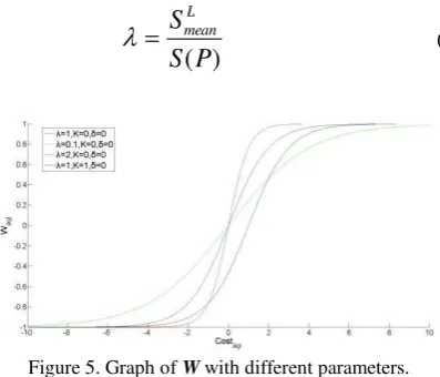
(11)The graph of Eq.(11) is shown in Figure 5. K describes the cost for the exact matching which is increased with the noise in the images. If PL is in discontinuities, we need a large to prevent
Figure 5. Graph of W with different parameters.
The graph of in different areas of Teddy is shown in Figure 6. A large which relates to discontinuities is brighter than a small one.
Figure 6. λ in different areas of Teddy.
Now E'' is calculated by Eq.(13) which is the objective function for optimization in Hopfield neural network (Hopfield, 1982). Neurons are based on the disparity space. Different connections of neurons indicate different assignments of disparities for each pixel. Neurons can not be self-connected and hence Wikik is 0.
The state of a neuron Pik is 0 or 1 which is calculated by the net.
Pikset to 1 implies that this neuron is active and the disparity of
the pixel Pi is k. When the state of a neuron changes from Pmn to
always falling during the updating of neuron states. The rule of updating is Eq.(16) (Nasrabadi and Choo, 1992). After a number of iterations, we obtain the minimum E' which relates to The International Archives of the Photogrammetry, Remote Sensing and Spatial Information Sciences, Volume XLI-B5, 2016
the required optimal disparity map.
ik ik N
j d
l
jl ikjl
ik N
j d
l
jl ikjl
ik N
j d
l
jl ikjl
P
P
P
W
P
P
W
P
P
W
,
0
1
0
,
0
1
1
,
0
1
1 1 1 1 1 1
max max
max
(16)
4. EXPERIMENTS AND EVALUATION
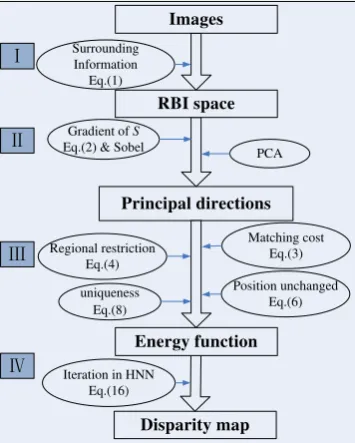
The workflow of our method is shown in Figure 7. First, we extract the surrounding information S of the input images and form our 3D RBI space to describe each pixel. Second we calculate the gradient of S and use PCA to obtain the principal directions of each pixel. Third, we calculate the matching cost, and add the constraints of the region, position and uniqueness to obtain the objective function. Finally, we solve the optimization problem by HNN. The output of HNN is the global minimum E which relates to the disparity map.
Disparity map Energy function Principal directions
Surrounding Information Eq.(1)
PCA
RBI space Images
Gradient of S
Eq.(2) & Sobel
Regional restriction Eq.(4)
Position unchanged Eq.(6) uniqueness
Eq.(8)
Matching cost Eq.(3)
Iteration in HNN Eq.(16)
Figure 7. The workflow of our method.
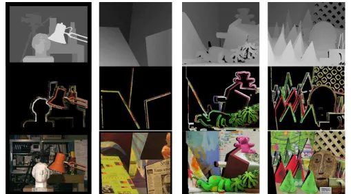
Images used for experiments are Tsukuba (384×288 pixels), Venus (434×383 pixels), Cones (450×375 pixels) and Teddy (450×375 pixels) from the Middlebury stereo benchmark (Scharstein and Szeliski, 2002). Figure 8 consists of the ground truth, discontinuities, and continuities for test dataset. The size of window N for the neighbor pixels in Eq.(1) depends on the size of featureless areas. In our experiment, N is 5 which balances the accuracy and time consumed. For the gradient of S, we extend the Sobel into 3D. We choose three principal directions from PCA to calculate the Eq.(3). For Eq.(4) and Eq.(12), the SL and SR are the surrounding RBI of PL's and PR's
adjacent pixels, respectively. We want to highlight the function
of discontinuities, thus w1 is 1 while w2 is 100. For η in Eq.(6),
is 1. Different images need different parameters, while for aforementioned images, these parameters work effectively.
The size of window N for the neighbor pixels in Eq.(1) depends on the size of featureless areas. In our experiment, N is 5 which balances the accuracy and time consumed. For the gradient of S, we extend the Sobel into 3D. We choose three principal directions from PCA to calculate the Eq.(3). For Eq.(4) and Eq.(12), the SL and SR are the surrounding RBI of PL's and PR's
adjacent pixels, respectively. We want to highlight the function of discontinuities, thus w1 is 1 while w2 is 100. For η in Eq.(6),
is 1. Different images need different parameters, while for aforementioned images, these parameters work effectively.
We conducted two experiments to validate the proposed method. First is to show the accuracy of the test images and the second is to illustrate the improvement of state-of-the-art methods by our algorithm.
The accuracy of compared methods and ours are shown in Table 1. In Table 1, con, all and dis denote the continuities, all areas and discontinuities, respectively. Results show that our method works pretty well, especially in discontinuities.
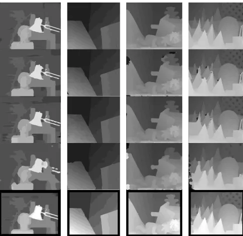
We compare our method with four discontinuities-preserving methods, including LLR, imprNLCA, Borders, and LCVB-DEM. We employ our method to improve other methods. This is convenient with less complexity, because the input for our method is just the discontinuous areas. As shown in Figure 9, all these methods are improved by our algorithm with respect to the accuracy of all areas and therefore, the bottleneck problem has been addressed effectively. Figure 10 shows the disparity maps of LLR, imprNLCA, Borders, LCVB-DEM and our results. From Figure 10, our results have an unambiguous discontinuous areas and less unmatched pixels which are shown as the 'black areas' on the disparity map.
5. CONCLUSIONS
This paper proposes an algorithm to preserve discontinuities in the disparity map. We form an energy function based on our novel 3D space. The discontinuity information is obtained from radial basis information. We calculate the difference of direction vectors for the cost of matching, and use the constraints of the region, position and uniqueness to reduce the search for a solution. To obtain the minimum cost, this function is deduced as an optimization problem which can be solved by HNN. By updating the neurons from the activation function, the global solution is generated automatically which is the optimal disparity map for the input images.
To evaluate our method, we show our results on the Middlebury benchmark. Our method outperforms state-of-the-art discontinuities-preserving methods, especially in terms of discontinuities. Apart from this, it can be used to augment other state-of-the-art approaches by preserving their discontinuities to solve the bottleneck of stereo matching.
Figure 8. Ground truth, discontinuities, and continuities. Ground truth (first row), discontinuities (second row), continuities (third row).
Method Tsukuba Venus Teddy Cones
con all dis con all dis con all dis con all dis
LLR 1.05 1.65 5.64 0.29 0.81 3.07 4.56 9.81 12.2 2.17 8.02 6.42
imprNLCA 1.38 1.83 7.38 0.21 0.41 2.26 5.99 11.5 14.3 2.85 6.68 7.93
Borders 1.29 1.71 6.83 0.25 0.53 2.26 7.02 12.2 16.3 3.90 9.85 10.2
LCVB-DEM 4.49 5.23 21.3 1.32 1.67 11.5 9.99 16.3 26.1 6.56 13.6 18.2
our method 1.18 1.79 4.89 0.20 0.47 1.91 4.82 9.84 11.3 6.07 9.47 6.34 Table 1. Comparison of results with error threshold 1.0
Figure 9. The improvement of start-of-the-art methods on all areas.
Figure 10. Results of different methods. LLR (first row), imprNLCA (second row), Borders (third row), LCVB-DEM (forth row) and our method (last row).
REFERENCES
Achour, K. and Mahiddine, L., 2002. Hopfield neural network based stereo matching algorithm. Journal of Mathematical Imaging and Vision,16(1), pp. 17–29.
Boykov, Y., Veksler, O. and Zabih, R., 2001. Fast approximate energy minimization via graph cuts. IEEE Transactions on Pattern Analysis and Machine Intelligence, 23(11), pp. 1222– 1239.
Buhmann, M. D., 2004. Radial basis functions: theory and implementations. Cambridge Monographs on Applied and Computational Mathematics, 12, pp. 147–165.
Chen, D., Ardabilian, M., Wang, X. and Chen, L., 2013. Animproved non-local cost aggregation method for stereo matching based on color and boundary cue. IEEE International Conference on Multimedia and Expo, pp. 1–6.
Cheng, F., Zhang, H., Sun, M. and Yuan, D., 2015. Cross-trees, edge and super-pixel priors-based cost aggregation for stereo matching. Pattern Recognition, 48(7), pp. 2269–2278.
Farid, H. and Simoncelli, E. P., 1997. Optimally rotation equivariant directional derivative kernels. Computer Analysis of Images and Patterns, pp. 207–214.
Hopfield, J. J., 1982. Neural networks and physical systems with emergent collective computational abilities. Proceedings of the National Academy of Sciences, 79(8), pp. 2554–2558.
Huang, C.-h. andWang, T.-h., 2000. Stereo correspondence using hopfield network with multiple constraints. IEEE International Conference on Systems, Man, and Cybernetics, Vol. 2, pp. 1518–1523.
Laskowski, Ł., Jelonkiewicz, J. and Hayashi, Y., 2015. Extensions of hopfield neural networks for solving of The International Archives of the Photogrammetry, Remote Sensing and Spatial Information Sciences, Volume XLI-B5, 2016
stereomatching problem. Artificial Intelligence and Soft Computing, pp. 59–71.
Lee, J. J., Shim, J. C. and Ha, Y. H., 1994. Stereo correspondence using the hopfield neural network of a new energy function. Pattern Recognition, 27(11), pp. 1513–1522.
Martins, J. A., Rodrigues, J. M. and du Buf, H., 2015. Luminance, colour, viewpoint and border enhanced disparity energy model. PloS one, 10(6), pp. 1-24.
Mattoccia, S., Tombari, F. and Di Stefano, L., 2007. Stereo vision enabling precise border localization within a scanline optimization framework. Asian Conference on Computer Vision, pp. 517–527.
Nasrabadi, N. M. and Choo, C. Y., 1992. Hopfield network for stereo vision correspondence. IEEE Transactions on Neural Networks, 3(1), pp. 5–13.
Ogale, A. S. and Aloimonos, Y., 2005. Shape and the stereo correspondence problem. International Journal of Computer Vision, 65(3), pp. 147–162.
Scharstein, D. and Szeliski, R., 2002. A taxonomy and evaluation of dense two-frame stereo correspondence algorithms. International Journal of Computer Vision, 47(1-3), pp. 7–42.
Sun, J., Zheng, N.-N. and Shum, H.-Y., 2003. Stereo matching using belief propagation., IEEE Transactions on Pattern Analysis and Machine Intelligence, 25(7), pp. 787–800.
Tombari, F., Mattoccia, S. and Di Stefano, L., 2007. Segmentation-based adaptive support for accurate stereo correspondence. Advances in Image and Video Technology, pp. 427–438.
Yang, Q., 2012. A non-local cost aggregation method for stereo matching. IEEE Conference on Computer Vision and Pattern Recognition, pp. 1402–1409.
Zhu, S., Zhang, L. and Jin, H., 2012. A locally linear regression model for boundary preserving regularization in stereo matching. European Conference on Computer Vision, pp. 101– 115.