OPTIMIZATION OF DECISION-MAKING FOR SPATIAL SAMPLING IN THE NORTH
CHINA PLAIN, BASED ON REMOTE-SENSING A PRIORI KNOWLEDGE
Jianzhong Feng a, c, *, Linyan Bai b, Shihong Liu a, c, Xiaolu Su c, Haiyan Hu c
a
Key Laboratory of Agri-information Service Technology, Ministry of Agriculture, Beijing, 100081, China -
[email protected]
b
Center for Earth Observation and Digital Earth Chinese Academy of Sciences, Beijing, 100101, China -
[email protected]c
Institute of Agriculture Information, Chinese Academy of Agricultural Sciences, Beijing 100081, China –
[email protected]
Commission VII, WG VII/4
KEY WORDS: Agricultural Spatial Sampling, Remote Sensing, a Priori Knowledge, Spatial Structure Characteristics, RIP(s)/RIV(s), Sampling efficiency
ABSTRACT:
In this paper, the MODIS remote sensing data, featured with low-cost, high-timely and moderate/low spatial resolutions, in the North China Plain (NCP) as a study region were firstly used to carry out mixed-pixel spectral decomposition to extract an useful regionalized indicator parameter (RIP) (i.e., an available ratio, that is, fraction/percentage, of winter wheat planting area in each pixel as a regionalized indicator variable (RIV) of spatial sampling) from the initial selected indicators. Then, the RIV values were spatially analyzed, and the spatial structure characteristics (i.e., spatial correlation and variation) of the NCP were achieved, which were further processed to obtain the scale-fitting, valid a priori knowledge or information of spatial sampling. Subsequently, founded upon an idea of rationally integrating probability-based and model-based sampling techniques and effectively utilizing the obtained a priori knowledge or information, the spatial sampling models and design schemes and their optimization and optimal selection were developed, as is a scientific basis of improving and optimizing the existing spatial sampling schemes of large-scale cropland remote sensing monitoring. Additionally, by the adaptive analysis and decision strategy the optimal local spatial prediction and gridded system of extrapolation results were able to excellently implement an adaptive report pattern of spatial sampling in accordance with report-covering units in order to satisfy the actual needs of sampling surveys.
* Corresponding author.
1. INTRODUCTION
For a long time, cropland area estimate using remote sensing technique is an important research topic of accurately estimating large-area crop yields by remote sensing approaches (Wang et al., 2008). It is very important for macro-economic decision-making departments of governments to timely know the related crop production and make scientific and sound decisions, etc. Spatial sampling technology is used to be able to effectively resolve this problem that a balance is realized between the cropland area accurate estimation and limited investigation budget (Li et al., 2004). It is essential for spatial sampling that the basic principles and methods of statistical sampling are applied to the regionalized attributes of geographical objects. Therefore, there are the probability spatial sampling techniques, based on traditional statistics, (such as simple random, systematic, stratified, and cluster spatial sampling) and model spatial sampling that are tied to spatial variability theory (Stevens Jr. and Olsen, 2004; Li et al., 2004; Dobbie and Henderson, 2008; Jia et al., 2008; Jiang et al., 2009). Due to the complexity of geographical features in a region, the traditional large-scale spatial sampling of resources or environmental investigation (especially on agricultural monitoring with remote sensing) are operated not well to use the a priori knowledge or information of spatial structure characteristics of some research region, but, relied on a certain sampling schema,
more often to use common probability sampling models and methods, such that they cannot meet actual requirements of spatial sampling investigation because their sampling efficiencies are not very high and ranges of sampling application are not large (Jiao et al., 2002, 2006; Wu et al., 2004).
In this paper, founded upon an idea of rationally integrating probability-based and model-based sampling techniques and properly using the relevant sampling models and methods, the valid spatial sampling design was developed in the North China Plain (NCP) as a study region, which is associated with remote sensing a priori knowledge or information, and the existing spatial sampling schemes were suggested to improve and optimize in better order to service the large-scale cropland remote sensing monitoring in the NCP. In short, this study can further effectively enhance the level of spatial sampling survey and decision-making analysis of the related departments of national and local governments.
2. METHODOLOGY
2.1 Models of a priori information acquisition
Geographical spatial structure characteristics are represented with the spatially correlated and heterogeneous properties of regionalized geographical elements (of surface things or phenomena) (Feng, 2010).
A fundamental approach of quantitatively describing spatial correlation makes use of the global and local spatial autocorrelation statistics (Anselin, 1988) that present the spatial dependencies of regionalized proximity objects with their indicator parameter(s)/variable(s) (RIP(s)/RIV(s)) in geographic space, which leads to the corresponding spatial two order effects of the RIP(s)/RIV(s). The former measures an overall spatial dependency of objects in a geographic space and the latter probes into the relational heterogeneous characteristics (variations) of geographic objects. Since the RIP/RIV (i.e., percentage of winter wheat planting area in each pixel), extracted from remote sensing images, of spatial sampling in this study was a variable, i.e., function of distances between spatial locations, the three statistics of Moran’s I, Geary’s C (Cliff and Ord, 1981) and General G (Getis and Ord,1992) were used to serve as available statistics of describing global/local spatial autocorrelation of the geographic RIP/RIV.
Given that variability and direction of stability of spatial correlations cannot effectively be explored using global and local autocorrelation measures, semivariance function and semivariogram, being concerned with a technique of exploratory spatial data analysis, are often used to clarify spatial heterogeneous properties, and they can obviously show spatial structure characters of geographic RIP(s)/RIV(s) (i.e., dependencies of which are dominantly described) and are thus very important tools of geographic spatial analysis (Zhuang, 2005; Wang et al., 2005; Ma et al., 2007). Regionalized variation function analysis is implemented under the second order (pseudo-)stationary hypothesis and/or the (pseudo-) intrinsic hypothesis, which easily results in having the experimental semivariance function below:
( ) of locations separated by a vector h (also called lag distance). a theoretical semivariance ( )h can be fitted using a set of values of an experimental semivariance and the relative models such as a linear, spherical, exponential and/or Gaussian model and its associated semivariogram be obtained, a shape of which represents spatial structuring (or correlation properties ) of variable Z x( ). There are three key parameters of sill (CC0),
rang (a) and nugget (C0) with respect to a ( )h
(semivariogram) that is generally a function of lag h. At a large separation distance (a) of h, the semivariogram reaches a plateau sill and the related values of Z x( ), separated by more
than h, are considered spatially independent, i.e., uncorrelated. Those are greatly significant for spatial sampling plan (including sample size design and sample-point separated distance determination, etc.) and its optimization because of collecting non-redundant samples being separated with at least the range of correlation apart. A C0 is connected with the
discontinuity behaviour of a semivariogram near the origin. It reflects the continuity of Z x( ) , which is related to either
uncorrelated noise (measurement error) or to spatial structures at spatial scales smaller than the pixel size, and therefore, the pertinent nugget effects in this study were neglected.
2.2 Spatial Sampling Design Optimization
There is a general spatial-sampling paradigm for a regional space (or subspace) that in the first place we should analyze its spatial structure characteristics (i.e., the correlation and variation of RIP(s)/RIV(s) of a sampling (sub-)population) as a priori knowledge/information of spatial sampling, and then decide a sample size, allocate sample-point locations, and estimate the total values of and means of and variances of sample and (sub-) population and so on, in order to obtain a optimal sampling solution.
Using the RIP(s)/RIV(s) of remotely sensed satellite imagery to carry out gridded spatial sampling, we considered resolution-level based gridding cells as sampling population units. There is a basic principle to find out the unstationary of and influencing ranges of local spatial procedures for the RIP(s)/RIV(s) betaking the local spatial autocorrelation statistics (such as
’ i sample-point sizes (scales) of sampling space (or subspace). Hence, this could avoid the local spatial dependency (correlation) to a certain extent and (approximately) suit the independent principles of sampling objects in classical statistic sampling theory, and then offer a series of selective schemes of designing a minimum sample-point size of spatial sampling plan. Subsequently, we were able to obtain a relatively optimal design of sample-point size by comparing them.
A global spatial autocorrelation measure is often founded under the spatial stationary condition, that is, the expectation and variance of the RIP(s)/RIV(s) of spatial objects in a geographic space are constant. Although the stationary of global spatial procedures does not exist in the real world (i.e., unstationary) and even more the hypothesis of spatial stationary is really very impossible, especially when the data of population being very huge (Ord and Getis, 1995; Anselin, 1995), the global spatial autocorrelation can approximatively display the spatial distribution of and trend characteristics of a whole population space (or subpopulation) with the RIP(s)/RIV(s). Thus the regionalized spatial structure characteristics are represented in terms of different perspectives of global spatial autocorrelation and regionalized spatial variation measures, respectively, which present the basis of application for sample-point allocation design of spatial sampling.
It is essential for the Kriging methodology (Atkinson et al., 1999a; Atkinson et al., 1999b; Journel, 1978) that an unknown value Z xv( 0) of a continuous variable is unbiasedly estimated
by the known values Z xv( )i (i1, 2,...,n) of a variable in object space using linear model, accuracy of which is determined by the variogram function of Kriging (Hou and Huang, 1990; Wang et al., 1990; Zhuang, 2005). Ordinary Kriging technique is an important type of the Kriging technology, a basic idea of which is to employ Kriging blocks (that is, values of local ranges) to estimate values of a bigger range. So, based on its principles and methods, a set of valid Kriging optimizing models and algorithms of regionalized spatial sampling is easily built (Li et al., 2004). 2.3 Adaptive Analysis and Decision Strategy
In this study, using the RIP/RIV (fraction/percentage of winter wheat planting area in each pixel) of remote sensing images and analyzing its spatial structure characteristics (spatial correlation and variation) as a priori knowledge/information, the spatial sampling was performed, depending on the multi-stratified International Archives of the Photogrammetry, Remote Sensing and Spatial Information Sciences, Volume XXXIX-B8, 2012
model mentioned above and the grid cells (i.e., pixels or multiplied pixels) as sampling objects of population. The sampling results (e.g., the total estimation and mean of sample/population) were gridded for different levels of administrative report units (such as province, county and township) to adaptively report in order to make scientific, helpful related decision (Wang et al, 2002; Feng, 2010). To estimate the total value, related mean and variance of regionalized population space (or its each subarea) and obtain adaptive inference, a set of valid Kriging optimizing models and algorithms of regionalized spatial sampling (Li et al., 2004; Feng, 2010) may be employed to predict the locally optimal RIP/RIV of spatial locations. There is a basic equation, as shows below:
1 is the RIP/RIV of a random sampling object at location xi of subarea Zzk, and n is the number of a sample, where zk( )xi is the proximate (adjacent) weight at xi and
1
a unbiased estimation (namely the expectation of prediction error E Z[ zkZˆzk]0 ). We can calculate all the unknown RIP/RIV’s values in zk using the least-squares method and draw out their associated spatial distribution plot through which the total value (or mean) of sampling population space is obtained by an accumulation approach. By betaking the Lagrange multiplier method, the minimum (Kriging) variance is able to obtain making use of the previous Kriging optimizing technique, which is related to the semivariogram of sampling space and distribution of sampling locations, but not to the RIP/RIV’s values of sample locations, and these are greatly merited and significant for the design of spatial sampling and its optimization.
3. DATA AND REGION OF STUDY
3.1 Region of Study
The North China Plain, also called Huang-Huai-Hai Plain, being the second plain (accounting for about one third of the whole plain area) in China, is situated with a range of about 32-40˚N, 114-121˚E. The plain covers an area of more than 380,000Km2, most of which is less than 50m above sea level, and it can, generally, be divided into three type units of the piedmont sloping plain, alluvial plain and coastal plain and is one of the most main regions for grain production in China. From an administrative district perspective, it includes the municipalities of Beijing and Tianjin, the provinces of Henan, Hebei, and Shandong provinces, merging with the Yangtze delta in northern Jiangsu and Anhui provinces, in which there are more than 320 counties (Gong, 1985; Huang et al., 1999; Liu et al, 2009; http://baike.baidu.com/view/416642.htm). Its dominant land-use type is cropland wherein more than 10 kinds of crops are grown, such as winter wheat, maize, millet, rice, peanut, sugar beets, and cotton.
3.2 Data and Processing
In this study, a scene CBERS-02 (China-Brazil Earth Resources Satellite program, the second satellite) CCD (Charge-coupled Device) image in spatial resolution of 19.5m, which covered a extent (35.07-36.29˚N, 114.3-115.82˚E) of original 7270 x 6930 pixels centered at 35.6905˚N, 115.068˚E on 2005-04-04 was obtained from the site (http://www.cresda. com/index.php) of China Centre for Resources Satellite Data and Application (CRESDA). Its corresponding surface area was located in the central part of North China Plain (CNP), which was one of main producing areas of winter wheat, and given a geographic representativeness of this area, its landscape features could appropriately represent the geographic characteristics of the whole CNP. After the chosen image was pre-processed (e.g., geometric calibration, cloud clearing, atmospheric corrections), it was aggregated into a expedient modeling image with a spatial resolution of 253.5m (about 250m) as a datum source of the following mixed-pixel spectral decomposition. Comparing the results of mixed-pixel spectral decomposition using the linear decomposition, fuzzy C-means clustering, BP (back propagation) neural network and support vector machine models, their most optimal model and method had been chosen. We selected the MODIS (Moderate Resolution Imaging Spectroradiometer) data including the ESWIR 8-day and EVI, Red, NIR and Blue 16-day composite Level 3 products from 2003-10 to 2004-06 over the CNP. Then, they were processed using the image-mosaicking, data phase-matching, and second order principal component analysis (PCA) (based on corresponding-time and multi-temporal data) techniques, wherein the spatial resolution of 250m was regarded as a baseline resolution, and were consequently incorporated into a scene as the available datum source in order to retrieve the fraction/percentage (as the spatial sampling RIP/RIV) of crop (i.e., winter wheat) planting area in its each pixel by betaking the above most optimal model and method of mixed-pixel spectral decomposition (See Table 1 and Appendix: Figure 1).
4. RESULTS AND ANALYSIS
4.1 Determining Sample Point Size
In this study, the RIP/RIV (i.e., percentage of winter wheat planting area in each pixel) distributing maps were the basic operated data in spatial resolution of 250m×250m used to determine a sample-point (i.e., sample-grain) minimum (baseline) scale. According to a series of sample-grain scales from 250m×250m to 2500m×2500m (where each scale-step difference was 250m), we analyzed the correlation characteristics of the NCP with the three local spatial autocorrelation statistics of Moran s I’ i, Geary s C’ i and Getis ord Gi (Genearal G: Gi或
*
i
G ) and then calculated their means, respectively. The corresponding increments (first order differences, namely differences of two adjacent statistic means) of the three means are shown in Figure 2.
We can find out the two difference sequences of Moran s I’ i and Getis ord Gi monotonously increasing in contrast to that of
’
Geary s Ci monotonously decreasing, and there are three principal turning points nearby at the sample-grain scale of 750m, which indicate that there was evident variation as to the autocorrelation mean characteristics in this study region, and International Archives of the Photogrammetry, Remote Sensing and Spatial Information Sciences, Volume XXXIX-B8, 2012
Table 1. Accuracy evaluation of mixed-pixel spectral decomposition of the CNP MODIS imagery
Sensor Name Spatial resolution m
Mean (%)
Variance ((%)2)
absolute error (%)
Relative Error (%)
EOS-MODIS 250 24.1295 59.1619
0.1543 0.6436
CBERS02-CCD 19.5 23.9752 29.8883
Figure 2. First order differences of means of local spatial autocorrelation (Getis ord Gi, Moran's Ii, Geary's Ci) under
difference spatial-sampling grains in the CNP, based on the fraction of winter-wheat planting area in each pixel (RIP/RIV) that is an important reference factor for sample point size design of spatial sampling. In addition, it was thinking of the spatial structuring and resolution of available MODIS images of the CNP and real feasibility of spatial sampling that the scale 750m×750 was determined as an optimal (optimum) sample-point size in spatial sampling of winter wheat area estimation of this study. This is consistent with the sample-point size of 500m×500m that is adopted currently in the actual cropland area remote sensing operation monitoring of winter wheat in North China plain. Given the research results, we may appropriately improve the existing sampling designs and implementing solutions so as to reduce the cost of spatial sampling for crop remote sensing monitoring and improve the spatial sampling efficiencies.
4.2 Determining Sample Point Distances
Distances between sample points (namely, sample-point distances) are important elements of spatial sampling design and can set up a set of sample points in all sampling space to a certain extent to be characterized and determine the implementation characteristics of corresponding spatial sampling. For example, distances of sample points, if too small, are likely to present the strong spatial correlations and then lower the adequately random characteristics of samples which are necessary of probability spatial sampling; being under certain sample size conditions, if too large, there are some difficulties to lay sample points in a sampling space, or, deficiencies that aren’t able to effectively use a priori knowledge or information (e.g., its spatial structuring) or fully represent the entire population features with samples (even though only using simple probability sampling methods). Hence, there are inevitably larges deviations between the sampling results and real populations and they further lower the efficiencies of spatial sampling. As a result, we should not only settle rational sample-point sizes but also arrange them being divided with reasonable intervals (i.e., sample-point distances), especially based on the minimum optimum intervals that are derived from spatial structuring in a sampling population space and the most foundational control requirement of implementing spatial sampling.
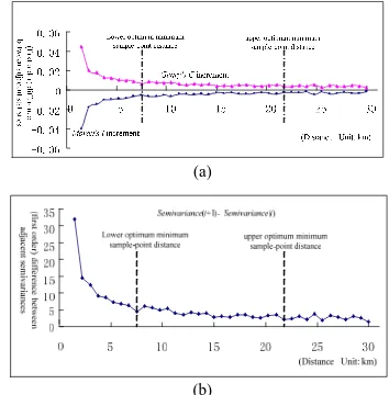
Therefore, global spatial autocorrelation analysis of the RIP(s)/RIV(s) of objects of sampling space is an useful method to explore the total spatial structure characteristics (including average correlation of and spatial distribution pattern of objects,
and significant degree of correlation, etc.) of a study region, based on the Moran's I and Geary's C and semivariogram analysis. In this study, the corresponding absolute change rates of the Moran's I, Geary's C and semivariogram representing the CNP’s spatial structure characteristics have the decreasing trend along a horizontal axis direction (See Figure 3), whereas there exists a greatly distinct turning point nearby at a lag of 7.5km and then their changes in size is very small, which indicates that sensitivities of this change trend are falling down along with increasing lags (i.e., separating distances among spatial objects). Besides, another distinct turning point appears at a lag of 22.5km, whereafter this trends to a more random stationary status. Consequently, we could settle the separating distances (from about 7.5 to 22.5km) as the sample-point distances because they were able to reach the pre-requisite minimum distances among sample points to reduce their spatial correlations to enough small degree and satisfy probability-sample random of and meanwhile, simultaneity certain accuracy requirements of spatial sampling. The results are consistent with the set sample-point distances (about 20~30km) of the current large-area operating spatial sampling survey of crop remote sensing monitoring in China North.
(a)
(b)
Figure 3. First order differences of (a) global spatial autocorrelation (Moran's I, Geary's C) and (b) semivariance
with sample-point separating distances, respectively 4.3 Spatial Sampling by Stratifying Spatial Autocor-relation Statistics
Given that we determined 750m×750m as an optimum pre-sample-point scale in the CNP, now the RIP/RIV (i.e., percentage of winter wheat planting area in each pixel) distributing maps in spatial resolution of 750m×750m served as the basic operated data by aggregating the baseline MODIS images (with spatial resolution of 250m×250m). Through local spatial autocorrelation analysis with the Moran’s Ii, Geary’s Ci
and Getis ord Gi (or Gi*), the results were obtained and
appropriately stratified, respectively. We could thus determine the corresponding average minimum sample-point distances of International Archives of the Photogrammetry, Remote Sensing and Spatial Information Sciences, Volume XXXIX-B8, 2012
each stratum subpopulation in light of one’s own spatial variability of each stratum.
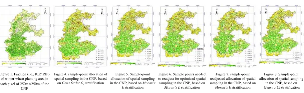
As Appendix: Figure 4 is shown, the total population was divided into six strata in terms of the Getis ord Gi, and a
proportion (percentage) of winter wheat planting area in this study region obtained by spatial sampling (computation) is 42.98 (%) and its relative error of -1%. Additionally, the result of integrating the sample point distributions in all the strata subpopulations by overlay operation shows that the total sample-point distances are not less than the corresponding average minimum sample-point distances of each stratum subpopulation and the previous obtained optimum synthetic sample-point distances (7.5km~22.5km). This could obtain a random sample and meet the requirement of probability random spatial sampling, so the sample point layout didn’t need to be readjusted and optimized.
Appendix: Figure 5 shows that, based on the Moran’s Ii, the
total population was also divided into six strata, and a proportion (percentage) of winter wheat planting area in this study region is 50.78 (%) and its relative error of 3.9%. Nevertheless, the result of integrating the sample point distributions in all the strata subpopulations by overlay operation illustrate that parts (which had 14 sample-point pairs checked as for the six strata) of the total sample-point distances are less than the above optimum synthetic sample-point distances (7.5km~22.5km) (See Appendix: Figure 6). Thus they didn’t meet the requirement of probability random spatial sampling and the sample point layout needed to be readjusted and optimized in order to make them not less than the optimal synthetic distances. Appendix: Figure 7 shows the results of the readjusted and optimized sample point distribution, and through computation a proportion (percentage) of winter wheat planting area in this study region is 50.897(%) and its relative error of 4.1%. Although its relative accuracy was reduced somewhat, still in an actually acceptable scope had it considerably well accuracy falling within more than 95%, and even more importantly, it made the sample-point spatial layout more reasonable and more geographically representative for probability random spatial sampling.
Using the Geary’s Ci, Appendix: Figure 8 shows that the total
population was divided into four strata, and a proportion (percentage) of winter wheat planting area in this study region is 42.05 (%) and its relative error of -14%. As is the same as that above of the Getis ord Gi, its sample point spatial distribution
could meet the requirement of probability random spatial sampling and didn’t thus need to readjust and optimized.
5. DISCUSSION
In order to provide adaptive analysis and reporting according to report units (such as province, county, township), based upon spatial structuring a priori knowledge/information, the Kriging spatial sampling technique(Feng, 2010) can be used to implement optimal local spatial prediction (i.e., extrapolation) and infer regionalized element population, whereafter inference result is gridded on basis of sampling grid basic cells and a data field map of regionalized elements of spatial sampling of study areas (that is, called a data field of spatial elements) is thus obtained. According to practical reporting needs, adaptive reporting patterns are able easily to perform using the obtained data fields and selected reporting units, depending on map
algebra of GIS (Geographical information systems, such as ARCGIS and MAPINFO).
Additionally, it is greatly important that remote sensing a priori knowledge/information (e.g., spatial structuring features) collaboratively associating with other pertinent helpful (a priori) knowledge or information (such as the relevant historical data of, spatial probability distribution mode of sampling objects of and traffic accessibility of study areas) is used in a spatial sampling procedure, which can more effectively improve efficiency, effectiveness and accuracy of spatial sampling. This is a research direction of our follow-up work.
6. CONCLUSIONS
In this paper, the MODIS remote sensing data, featured with low-cost, high-timely and moderate/low spatial resolutions, in the NCP as a study region were firstly used to carry out mixed-pixel spectral decomposition to extract an useful RIP/RIV from the initial selected indicators. Then, the RIV values were spatially analyzed, and the spatial structure characteristics (i.e., spatial correlation and variation) of the NCP were achieved, which were further processed to obtain the scale-fitting, valid a priori knowledge or information of spatial sampling. Subsequently, founded upon an idea of rationally integrating probability-based and model-based sampling techniques and effectively utilizing the obtained a priori knowledge or information, the spatial sampling models and design schemes and their optimization and optimal selection were developed, as is a scientific basis of improving and optimizing the existing spatial sampling schemes of large-scale cropland remote sensing monitoring. In addition, in terms of the adaptive analysis and decision strategy, the optimal local spatial prediction and gridded system of extrapolation results were able to excellently implement an adaptive reporting pattern of spatial sampling in accordance with report-covering units in order to satisfy the actual needs of researches or running operation of sampling surveys. This study can further effectively enhance the level of spatial sampling survey and decision-making analysis of the pertinent departments of national and local governments.
ACKOWLEDGEMENTS
This work was supported by the China National Science Foundation (No. 41171340, 41101390) and China National 863 Project(No. 2006AA120103).
REFERENCES
Anselin L., 1995. Local Indicators of Spatial Association: LISA. Geographical Analysis, 27(5), pp. 93-115.
Anselin, L., 1988. Spatial Econometrics: Methods and Models. Boston: Kluwer Academic Publishers.
Atkinson P. M. and D. R. Emery, 1999a. Exploring the relation between spatial structure and wavelength: Implications for sampling reflectance in the field. International Journal of Remote Sensing, 20, pp. 2663-2670.
Atkinson P. M., 1999b. Geographical information science: Geostatistics and uncertainty. Progress in Physical Geography, 23, pp. 134-140.
Cliff, A. D., and J. K. Ord, 1981. Spatial Processes: Models & Applications. London: Pion.
Dobbie M. J and B. L. Henderson., 2008. Sparse sampling: Spatial design for monitoring stream networks. Statistics Surveys, 2, pp. 113-153.
Feng Jianzhong, 2010. Spatial sampling theory and methodology based on remote-sensing a priori knowledge. Insitute of Agricultural Resources and Regional Planning, Chinese Academy of Agricultural Sciences, Postdoctor Research Report.
Getis A. and Ord J. K., 1992. The analysi of spatial association by use of distance statitisc. Geographical Analyis, 23(3), pp. 189-206.
Gong G. Y., 1985. Treatment and development of the Huang-huai-hai Plain: Preliminary discussion of spatial scope about the Huang-huai-hai Plain (No. 1). Beijing: Science Press.
Hu J. R. and J. X. Huang, 1990. The theory and method of geological statistics. Beijing: geological publishing house, pp. 22-240.
Huang B. W., D. Zheng and M. C. Zhao, 1999. Modern nature geography. Beijing: Science Press, pp. 299-318.
Jia B., W. Q. Zhu, Y. Z. Pan, G. B. Song and T. G. Hu, 2008. Sensitivity Analysis of Pre-classification Accuracy Based on Remote Sensing Image to Ground Area Estimation from Spatial Sampling. Journal of Remote Sensing, 12(6), pp. 972-979. Jiang C. S., J. F. Wang and Z. D. Cao, 2009. A review of Geospatial sampling theory. Acta Geographica Sinica, 64(3), pp. 368-380.
Jiao X. F., B. J. Yang and Z. Y. Pei, 2002. Design of Sampling Method for Cotton Field Area Estimation Using Remote Sensing at a National Level. Transactions of the CSAE, 18(4), pp. 159-162.
Jiao X. F., B. J. Yang and Z. Y. Pei, 2002. Paddy rice area estimation using a stratified sampling method with remote sensing in China. Transactions of the CSAE, 22(5), pp. 105-110. Journel A. and C. H. Huijbregts, 1978. Mining Geostatistics. London: Academic Press Inc., pp. 1-150.
Li Lianfa, Wang Jinfeng, Liu Jiyuan, 2004. Optimization of decision-making for spatial sampling in remote sensing survey of land. Science in China (Series D), 34(10), pp. 975-982. Liu F. Y., J. H. Cui, L. J. Chen, Y. X. Zhao, Y. J. Qin and C. Wu, 2009. A View on Geomorphologic Zonalization of North China Plain. Geography and Geo-information Science, 25(4), pp. 100-103.
Ma R. H., Y. X. Pu and X. D. Ma, 2007. GIS spatial correlation patterns and exploring discovery. Beijing: Science Press, pp. 3-137.
Ord J. K. and A. Getis, 1995. Local spatial autocorrelation statistics: distribution issue and an application. Geographical Analysis, 27(4), pp. 286-306.
Stevens Jr. D. L. and A. R. Olsen, 2004. Spatially Balanced Sampling of Natural Resources. Journal of the American Statistical Association, 99(465), pp. 262-278.
Wang D., Q. B. Zhou and J. Liu, 2008. Studies on experiment of optimizing design of space sampling frame and sampling basic elements of crop area. Chinese Journal of Agricultural Resources and Regional Planning, 29(4), pp. 9-15.
Wang J. Y. et al., 1990. Geostatistics and its application in the development of coal resources. Beijing: China Coal Industry Publishing House, pp. 25-221.
Wang J., D. Zhuang, L. Li and Y. Ge, 2002. Spatial sampling design for monitoring the area of cultivated land. International Jouma1 of Remote Sensing, l3(2), pp. 263-284.
Wang X. J. et al., 2005. Spatial analysis of soil trace metal contents. Beijing: Science Press.
Wu B. F. and Q. Z. Li, 2004. Crop Acreage Estimation Using Two Individual Sampling Fram eworks with Stratification. Journal of Remote Sensing, 8(6), pp. 551-569.
Zhang R. D., 2005. The spatial variability theory and Application. Beijing: Science Press.
APPENDIX: RELATED FIGURES
Figure 1. Fraction (i.e., RIP/ RIP) of winter wheat planting area in each pixel of 250m×250m of the
CNP
Figure 4. sample-point allocation of spatial sampling in the CNP, based on Getis Order Gi stratification
Figure 5. Sample-point allocation of spatial sampling in the CNP, based on Moran’s
Ii stratification
Figure 6. Sample points needed to readjust for optimized spatial sampling in the CNP, based on
Moran’s Ii stratification
Figure 7. sample-point readjusted allocation of spatial sampling in the CNP, based on
Moran’s Ii stratification
Figure 8. Sample-point allocation of spatial sampling
in the CNP, based on Geary’s Ci stratification International Archives of the Photogrammetry, Remote Sensing and Spatial Information Sciences, Volume XXXIX-B8, 2012