EVALUATING THE EFFECTS OF REDUCTIONS IN LiDAR DATA ON THE VISUAL
AND STATISTICAL CHARACTERISTICS OF THE CREATED DIGITAL ELEVATION
MODELS
F. F. Asal a
a
Civil Engineering Department, Faculty of Engineering, Menoufia University, Shebin El-Kom, Egypt; [email protected]
Keywords: DEM/DSM/DTM, Airborne LiDAR, Point cloud density, Visualization, DEM quality, Elevation accuracy, Spatial
analysis.
ABSTRACT
With continuous developments in LiDAR technologies high point cloud densities have been attainable but accompanied by challenges for processing big volumes of data. Reductions in high point cloud densities are expected to lower data acquisition and data processing costs; however this could affect the characteristics of the generated Digital Elevation Models (DEMs). This research aimed to evaluate the effects of reductions in airborne LiDAR point cloud data densities on the visual and statistical characteristics of the generated DEMs. DEMs have been created from a dataset which constitutes last returns of raw LiDAR data that was acquired at bare lands for Gilmer County, USA between March and April 2004, where qualitative and quantitative testing analyses have been performed. Visual analysis has shown that the DEM can withstand a considerable degree of quality with reduced densities down to 0.128pts/m2 (47% of the data remaining), however degradations in the DEM visual characteristics appeared in coarser tones and rougher textures have occurred with more reductions. Additionally, the statistical analysis has indicated that the standard deviations of the DEM elevations have decreased by only 22% of the total decrease with data density reductions down to 0.101pts/m2 (37% of the data remaining) while greater rate of decreasing in the standard deviations has occurred with more reductions referring to greater rate of surface smoothing and elevation approximating. Furthermore, the accuracy analysis testing has given that the DEM accuracy has degraded by only 4.83% of the total degradations with data density reductions down to 0.128pts/m2, however great deteriorations in the DEM accuracy have occurred with more data reductions. Finally, it is recommended that LiDAR data can withstand point density reductions down to 0.128pts/m2 (about 50% of the data) without big deteriorations in the visual and statistical characteristics of the generated DEMs.
1. INTRODUCTION
Digital Elevation Model (DEM) plays an important role in a wide range of applications including terrain modeling, landscape modeling, and hydrological modeling (Liu and Zhang, 2008) which makes the quality of the DEM to be crucial for different spatial modeling techniques (Anderson et al., 2005, Habib et al. 2005). Different factors including the density and distribution of the source data, the interpolation algorithm and the grid resolution affect the accuracy of the DEMs (Watt et al. 2013). Traditional surveying methods such as ground surveying and photogrammetric techniques can give high accuracy terrain data, however they are time consuming and labor intensive (Bilskie and Hagen. 2013, Watt et al. 2013). Light Detection and Ranging (LiDAR) technology has been increasingly used as an effective alternative to conventional optical remote sensing methods in accurately estimating above ground features where LiDAR measures the ranges to distant objects through measuring the time delay between the moment of transmission of the laser pulse and the moment of detection of the reflected signal (Wehr and Lohr, 1999). Compared to the DEM derived from photogrammetric techniques LiDAR DEM is more reliable and more accurate (Watt et al. 2013, Guo et al., 2010, Liu and Zhang, 2008). The accuracy of LiDAR DEM is controlled by factors, such as topographic variability, sampling density, interpolation methods, spatial resolution, etc. (Liu et al., 2007). Continuous developments in LiDAR technology have made high point densities and improved data accuracies attainable. However, this has been accompanied by challenges for data storage, data processing and manipulation of large volumes of data (Singh et al. 2015, Liu et al., 2007). Reductions of such high point densities are expected to lower
data acquisition costs and overcome computational challenges in DEM generation (Singh et al. 2015). On the other hand, reductions in point densities are expected to have direct effects on the visual and statistical characteristics of the generated DEMs. However, if those effects on DEM characteristics due to data reductions are not that important for some applications, this could result in savings in data acquisitions and processing costs. Thus, a balance between the point density and the volume of data should optimize the cost of data acquisition, data storage and data processing time (Anderson et al., 2005).
that data density has a crucial impact on the accuracy of the DEM created from airborne LiDAR surveys where they created DEMs from a very high point-density LiDAR data and simulated lower point-density LiDAR collection through decreasing percentages of points. They compared the DEMs created from the lower point density datasets with the original data DEM. Their results indicated decrease in DEM accuracy due to reductions in the data resolution.
Watt et al. 2013 stated that, for forest assessment and analysis using LiDAR data, although relatively high pulse densities are required for creating a DEM, once this has been developed there is a scope for reducing pulse density on subsequent flights to estimate stand matrix for forest inventory from LiDAR. Marin et al. 2013 carried out a research for determining the accuracy that can be expected when using LiDAR data density of 0.5points/m2. They developed a methodology based on establishing control points on the tops of constructions and measuring elevations using GPS which were compared with their corresponding values extracted from LiDAR DEM. They recommended that low density LiDAR can determine elevations within accuracies of 10-25cm. Also, Singh et al. 2015 evaluated the effects of LiDAR point density on the biomass estimation of remnant forests in the rapidly urbanizing region of Charlotte, North Carolina, USA. They suggested that LiDAR data with an average point spacing of 0.70–1.50 m (approximately 1.35points/m2) might offer a cost-effective procurement and processing at large-area (Singh et al. 2015).
This research aims to evaluate the effects of reductions in LiDAR point cloud data densities on the visual and statistical characteristics of the generated digital elevation models (DEMs) since these reductions could lower the data acquisition and data processing costs. It also aims to answer the question to what extent LiDAR data can be reduced without sacrificing qualitative and quantitative characteristics of the reduced data DEM. Last returns raw LiDAR dataset acquired at bare lands for Gilmer County, USA between March and April 2004 and downloaded from the county website has been used in this analysis. Reductions have been performed randomly on the raw LiDAR data at different percentages to simulate lower density LiDAR data acquisitions. DEMs have been created from the raw LiDAR data and from the reduced LiDAR data using ESRI spatial analysis and 3-D analyst working under ArcView GIS commercial packages where the Inverse Distance Weighting (IDW) with the power of four and grid resolution of 0.50metres were used for all the generated DEMs. Qualitative analysis using 2D and 3D visual analysis of the DEMs has been undertaken aiming at viewing the effects of the LiDAR data reductions on the quality of mapping the earth’s surface. Also, statistical analysis has been carried out for the generated DEMs from the reduced data and compared with the DEM from the original LiDAR data. Moreover, profile testing has been examined at different positions of the test area. Finally, quantitative analysis through assessment of the accuracy of the extracted elevations from the DEMs using external checkout points as ground truth data has been performed.
2. TEST SITE AND DATASET
Figure 1 shows a sample of raw LiDAR data which constitutes the last returns acquired at bare lands for Gilmer County, USA between March and April 2004 and downloaded from the county website. The sample data consists of about 11,176 points and covers an area of about 159.5 metres by 259 metres (i.e. 41310.5 squared-metres giving point density of one point per 3.6964 m2 (0.2705pts/m2) The maximum and minimum
elevations are 382.34 and 329.13 metres respectively giving a range of elevations of 53.21metres. The mean elevation is 363.213metres while the median elevation is 365.34metres and the mode elevation is 369.43metres. The variance of the elevations is 103.6222m2 giving a standard deviation of the elevations as ± 10.1795m, which is high value referring to highly varied terrain. Reductions of the data have been carried out manually trying to preserve uniformity of the remaining data points all over the site area as possible using MS Excel and MS Access. Ten reduced data files of 9,940 (89.02%), 9,177l (82.11%), 8,407 (75.22%), 7,590 (67.91%), 6,439 (57.61%), 5,308 (47.49%), 4,170 (37.31%), 2,767 (24.76%), 1,529 (13.68%) and 722 (6.49%) points giving point densities of 0.2705, 0.240, 0.222, 0.203, 0.184, 0.156, 0.128, 0.101, 0.067, 0.037 and 0.017pts/m2 respectively. Figure 2 depicts the most reduced data file down to 0.017pts /m2 point cloud density.
Figure 1. The original raw LiDAR data of 0.2705pts/m2 point cloud density
Figure 2. Reduced raw LiDAR data down to 0.0175pts/m2 point cloud density
3. 2D VISUAL ANALYSIS OF THE DEMs CREATED FROM REDUCED POINT DENSITY LiDAR DATA
LiDAR data set of 0.2705pts/m2. Also, Figures from 4 to 10 represent DEMs generated from the reduced data at different percentages giving point cloud densities of 0.222, 0.184, 0.128, 0.101, 0.067, 0.037, and 0.017pts/m2 respectively.
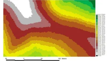
Figure 3. DEM generated from the original LiDAR data of 0.2705pts/m2 point cloud density.
Figure 4. DEM created from reduced LiDAR data down to point cloud density of 0.222pts/m2.
Figure 5. DEM created from reduced LiDAR data down to point cloud density of 0.184pts/m2.
Figure 6. DEM created from reduced LiDAR data down to point cloud density of 0.128pts/m2.
Very small but increasing differences can be visually interpretable between Figure 3, the DEM generated from the original LiDAR dataset and Figures 4, 5 and 6 which are DEMs generated from reduced LiDAR data down to point cloud
densities of 0.222, 0.184 and 0.128pts/m2 respectively. This can be observed in increasing of the corrugations of the borders separating the different colour classes, which refers to increasing in coarser tones and rougher textures. The changes in the patterns in the DEMs are hardly noticeable with almost any existence of tinny colour patches as indications of negligible losses of details due to data reductions down to point density of 0.128pts/m2.
Figure 7. DEM created from reduced LiDAR data down to point cloud density of 0.101pts/m2.
Figure 8. DEM created from reduced LiDAR data down to point cloud density of 0.067pts/m2.
Figure 9. DEM created from reduced LiDAR data down to point cloud density of 0.037pts/m2.
which are DEMs generated from reduced point densities down to 0.037 and 0.017pts/m2. This refers to increasing in terrain smoothing and elevation approximating. Thus, it can be recommended that the DEM visual characteristics can withstand a considerable degree of quality with reductions in LiDAR data down to point density of 0.128pts/m2 (about 50% of the data); however deteriorations in these characteristics have to be expected when omitting more than 50% of the original data.
Figure 10. DEM created from reduced LiDAR data down to point cloud density of 0.017pts/m2.
4. 3D VISUALIZATION OF THE DEMs CREATED FROM REDUCED POINT DENSITY LiDAR DATA
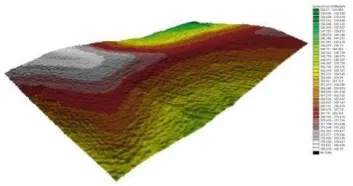
3D visual analysis has been undertaken so that the changes in the visual characteristics of the DEMs due to reductions in LiDAR point cloud data density can be 3D viewed and become more sensible. As followed in the 2D visual analysis the elements of the digital image interpretation have been employed in this analysis. Figure 11 represents a 3D view for a DEM generated from the original raw LiDAR data. Also, Figures from 12 to 18 depict 3D views for DEMs generated from reduced LiDAR data down to point cloud densities of 0.222, 0.184, 0.128, 0.101, 0.067, 0.037, and 0.017pts/m2 respectively.
Figure 11. 3D view for a DEM created from the original LiDAR data of point cloud density of 0.2705pts/m2.
Figure 12. 3D view for a DEM created from reduced LiDAR data down to point cloud density of 0.222pts/m2.
Small differences in the tones and textures can be interpreted between Figure 11; the 3D view for the DEM from the original data and Figures 12, 13, and 14 which are 3D views for the
DEMs generated from reduced point cloud densities down to 0.222, 0.184, 0.128pts/m2 respectively. Also, the reduced data 3D views almost have kept similar patterns to those in the original data 3D view despite reductions in LiDAR point cloud data density.
Figure 13: 3D view for a DEM created from reduced LiDAR data down to point cloud density of 0.184pts/m2.
Figure 14. 3D view for a DEM created from reduced LiDAR data down to point cloud density of 0.128pts/m2.
Figure 15. 3D view for a DEM created from reduced LiDAR data down to point cloud density of 0.101pts/m2.
Figure 16. 3D view for a DEM created from reduced LiDAR data down to point cloud density of 0.067pts/m2.
corrugated 3D views with increases in the sizes and shapes of the corrugations. This means that with lower point cloud densities great approximations in the extraction of the ground elevations have occurred. 3D visualization gives more sensible interpretation to what extent LiDAR point cloud data can be reduced with keeping a considerable degree of quality for the DEM visual characteristics.
Figure 17. 3D for a DEM created from reduced LiDAR data of point cloud density down to 0.037pts/m2.
Figure 18. 3D view for a DEM created from reduced LiDAR data down to point cloud density of 0.017pts/m2.
5. STATISTICAL ANALYSIS OF THE DEMs CREATED FROM REDUCED POINT CLOUD
LiDAR DATA
Tables 1a and 1b depict the results of the statistical analysis of the DEM generated from the original raw LiDAR data of point cloud density of 0.2705pts/m2 in addition to the DEMs generated from reduced LiDAR data down to 0.222, 0.184, 0.128, 0.101, 0.067, 0.037, and 0.017pts/m2 point cloud densities respectively. The results of the statistical analysis show that the number of rows, the number of columns and the number of cells (the count) keep same values; 319, 518 and 165242 respectively for all DEMs since the grid cell sizes are same for all DEMs (0.50m).
Statistic. Quantity
DEM of 100%
DEM of 82.11%
DEM of 67.91%
DEM of 47.49% Density.
(pts/m2) 0.2705 0.222 0.184 0.128
Max. (m) 382.337 382.337 382.337 382.250
Min. (m) 329.131 329.131 329.131 329.670
Mean(m) 362.387 362.387 362.388 362.387 Range
(m) 53.206 53.206 53.206 52.580
Sum (m) 59881498 59881554 59881711 59881624 Standard
Dev.(m) 10.193 10.191 10.190 10.187
Table 1a: The statistical analysis results of the DEMs created from reduced point cloud LiDAR data.
Statistic. Quantity
DEM of 37.31%
DEM of 24.76%
DEM of 13.68%
DEM of 6.49% Density.
(pts/m2) 0.101 0.067 0.037 0.017
Max. (m) 382.250 382.250 382.250 382.250
Min. (m) 329.670 329.670 329.890 329.670
Mean(m) 362.388 362.393 362.397 362.393 Range
(m) 52.580 52.580 52.360 52.580
Sum (m) 59881697 59882519 59883205 38224973 Standard
Dev. (m) 10.185 10.175 10.157 10.175
Table 1b. The statistical analysis results of the DEMs created from reduced point cloud LiDAR data.
Figure 19. The effects of reductions in LiDAR data on the ranges of the DEM elevations.
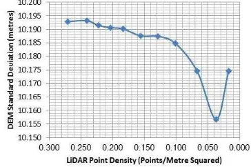
Figure 20. The effects of reductions in LiDAR data on the standard deviation of the DEM elevations.
and elevation approximating as results of missing of great parts of the data.
6. PROFILING FROM THE REDUCED DATA DEMs
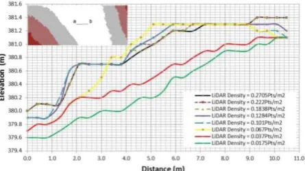
In this test the effects of reductions in LiDAR data are to be viewed vertically and the deviations of the reduced data profiles from the original data profile can be computed at different points of the profiles that can be extracted from different types of terrains. Figure 21 depicts a group of profiles extracted across the line a-b from the DEMs generated from LiDAR data of point cloud densities of 0.2705, 0.222, 0.184, 0.128, 0.101, 0.067, 0.037, and 0.017pts/m2 at a mildly varied terrain. Also, Figure 22 depicts another group of profiles generated along the line c-d from the same DEMs but at a corrugated terrain. From Figures 21 and 22 the profiles extracted from the DEMs of reduced data of densities down to 0.222, 0.184, 0.128, 0.101pts/m2 run very close to the profile extracted from the DEM of the original data that is of point cloud density of 0.2075pts/m2, (the black one) in both Figures. Deviations from the original data profiles increase significantly in the profiles from point cloud densities less than 0.101pts/m2. This is very
Figure 21. Profiles a-b extracted from DEMs created from LiDAR data of different point cloud densities.
Figure 22. Profiles c-d extracted from DEMs created from LiDAR data of different point cloud densities.
7. ACCURACY ANALYSIS OF THE DEMs CREATED FROM REDUCED POINT CLOUD LiDAR DATA DEMs where the residual elevations have been calculated using the following equations (Zhu et al. 2005, Karl et al. 2006):
δ = Elev.checkout– Elev.DEM (1)
where: δ = residual elevations.
Elev.checkout = elevation of the external checkout point. Elev.DEM = elevation from the DEM.
Then, the standard error σ of the residuals can be computed as:
√ (2)
Where: n = no. of observations (checkout points).
Statistical
0.199494 0.200488 0.200671 0.224633
Table 2a: Statistical analysis of the residuals of the elevations extracted from DEMs created from LiDAR data of different
point cloud densities at the positions of checkout points.
Statistical
0.307568 0.273157 0.443725 0.719036
Table 2b: Statistical analysis of the residuals of the elevations extracted from DEMs created from LiDAR data of different
point cloud densities at the positions of checkout points.
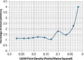
changes due to data reductions down to point density of 0.128pts/m2 however dramatic increases occur with more reductions. The mean residuals record slight changes with reductions in point densities down to 0.222pts/m2 with greater changes in their values occur with more reductions. Also, Figure 23, that depicts the relationship of the ranges of the elevation residuals against LiDAR point cloud density, shows dramatic increase in the ranges of elevations with point data densities lower than 0.128pts/m2 (47.49% of the data). Moreover, Figure 24 that represents the relationship of the standard errors of the elevation residuals against LiDAR point cloud data density, presents slight changes in the standard errors of the elevation residuals due to data reductions down to point density of 0.128pts/m2 to record only 4.83% of the total decrease, however big increases in the standard errors of the elevation residuals occur with more reductions which is indications of deteriorations in the accuracy of the extracted elevations. Thus, LiDAR data can withstand reductions down to 50% of the original data without sacrificing the DEM accuracy.
Figure 23. The ranges of the elevation residuals against LiDAR point cloud density.
Figure 24. The standard errors of the elevation residuals against LiDAR point cloud density.
8. DISCUSSIONS
The effects of LiDAR data reductions on visual and statistical characteristics of the DEMs have been investigated through five analysis tests namely; visual analysis, 3D visualization, statistical analysis and profiling from the reduced data DEMs, in addition to accuracy analysis of the elevations extracted from the DEMs produced from different point cloud densities. Visual analysis and 3D visualization have exploited the elements of the digital image interpretation to uncover the differences occurring in the DEMs due to reductions in the point cloud LiDAR data densities. Small but increasing differences have been visually interpretable between the original data DEM and the DEMs generated from reduced
LiDAR data down to 0.128pts/m2 that appeared in increasing of the border corrugations between different colour classes. More reductions in the point densities makes those differences to become more observables, see the DEM from data of 0.101pts/m2 point density where more corrugated colour class borders, coarser tones, rougher textures and pattern changes have been interpretable which means that great reductions in the point cloud density have produced degradations in the DEM visual characteristics due to terrain smoothing and elevation approximating. This has been similar to what extracted from the 3D visualization where, little changes in the tones and textures have been interpretable in the 3D views for the DEM from the original data and the 3D views of the DEMs generated from reduced data densities down to 0.128pts/m2, but with more reductions in the data, much coarser tones and rougher textures with random patterns have resulted. Thus, the visual characteristics of the DEM can withstand reductions down to 0.128pts/m2 (50% of the data) without clear degradations.
The statistical analysis results have interpreted the results of the visual analysis in numbers, showing that the maximum, the minimum elevations in the DEM and consequently the ranges of elevations have recorded little changes due to data reductions down to 0.184pts/m2 (67.91% of the original data), however dramatic decreases in their values occurred with more data reductions. Additionally, the standard deviations of the DEM elevations have decreased gradually and mildly with data reductions down to 0.101pts/m2 (37.31% of the data) while dramatic decreases have occurred with more data reductions referring to feature smoothing as results of missing of considerable parts of the LiDAR data. Moreover the profile testing has been undertaken so that the effects of the LiDAR data reductions on the DEM characteristics become more assessable. The profiles from the DEMs created from the reduced data files down to 0.101pts/m2, run very close to the original data DEM profile. However, clear positive and negative deviations from the original data profile increased significantly in the profiles from DEMs of point density lower than 0.101pts/m2 where the profiles from the DEM of point density of 0.017pts/m2 has showed the greatest deviations from the original data profile that can be as great as 0.80m. Also, at corrugated terrains the profiles from low data density DEMs run very disturbed around the original data profile.
The accuracy analysis test has given more understanding and clarification of the results obtained from the other four tests. The absolute maximum, minimum residuals and consequently the ranges of residuals have showed slight changes due to reductions in the point cloud data densities down to point density of 0.128pts/m2 (47.49% of the data), however dramatic increases in these statistical values occurred with more reductions. Also, the standard errors of the elevation residuals have kept very little changes, to recorded 4.83% of the total increase with data reductions down to 0.128pts/m2. On the other hand there have been dramatic increases in their values with more data reductions which means that LiDAR data can withstand data reductions down to about 50% of the data without great deteriorations in the accuracy of extracted elevations from the DEMs that expresses the DEM accuracy.
9. CONCLUSIONS
densities, to simulate low data density acquisitions. The created DEMs have been subjected to qualitative and quantitative analyses testing. Qualitative visual analysis testing has showed little changes in the tones and textures between the original data DEM and the reduced data DEMs down to 0.128pts/m2; however, lower point data density DEMs have shown much coarser tones and much rougher textures. Thus, visual characteristics of the DEM can withstand a considerable degree of quality with LiDAR data reductions down to about 50% of the original data. The maximum, the minimum and the ranges of elevations in the DEMs have kept very little changes with data reductions down to 67.91% while the standard deviations of the DEM elevations have recorded gradual but mild decrease recording 22% of the total decrease with reductions down to 37.31% of the data; however, dramatic decreases occurred with more reductions referring to feature smoothing and elevation approximation as results of missing of great parts of the original data. Additionally, the profiles extracted from the DEMs generated from reduced data down to 0.101 pts/m2 run close to the original data DEM profile while clear and increased positive and negative deviations from that profile have been observed in the profiles from the DEMs of lower point cloud data density than 0.101 pts/m2. The maximum, the minimum residuals and the ranges of residuals in addition to the standard errors of the residuals have kept slight changes with data reductions down to point density of 0.128pts/m2 (47.49% of the data); however, dramatic increases in their values have occurred with more data reductions. This means that LiDAR data can withstand data reductions down to about 50% of the original data without great deterioration in the DEM accuracy. In this research the method of IDW with power of four has been used for the creation of the DEMs from different point cloud density LiDAR data files. However, trying other interpolation approaches with different parameter variations could give better understanding of how the reductions in LiDAR point cloud data density would affect the visual and statistical characteristics of the generated digital elevation models.
ACKNOWLEDGMENTS
The author would like to acknowledge the three anonymous reviewers who have helped strengthening the paper.
REFERENCES
Anderson, E. S., Thompson, J. A. and Austin, R. E., 2005. LiDAR density and linear interpolator effects on elevation estimates. The International Journal of Remote Sensing, 26 (18), pp.3889-3900.
Bilskie, M. V. and Hagen, S. C. 2013. Topographic Accuracy Assessment of Bare Earth LiDAR-Derived Unstructured Meshes. Advances in Water Resources 52 (2013) 165-177 Elsevier.
Guo, Q., Li, W., Yu, H. and Alvarez, O. 2010. Effects of Topographic Variability and LiDAR Sampling Density on Several DEM Interpolation Methods. Photogrammetric Engineering & Remote Sensing Vol. 76, No. 6, June 2010,
Habib, A., Ghanma, M., Morgan, M. and Al-Ruzouq, R., 2005. Photogrammetric and LiDAR Data Registration Using Linear Features. Photogrammetric Engineering and Remote Sensing, 71 (6), pp.699-707.
Jensen, J. 2005. Introductory Digital Image Processing – a Remote Sensing Perspective. Third Edition. Pearson Prentice Hall, Upper Saddle River, New Jersey, 07458. USA.
Jensen, J. 2000. Remote Sensing of the Environment: An Earth Resource Perspective. Pearson Prentice Hall, Upper Saddle River, New Jersey 07458.
Karel, W., Pfeifer, N. and Briese, C. 2006. DTM Quality Assessment. Comm. II Symposium. Vienna; 12-14 July, 2006. International Archives of ISPRS, XXXVI/2, 1682-1750: 7 -12.
Lillesand, T. M. and Keifer, R. W. 2000. Remote Sensing and Image Interpretation. Fourth Edition, John Wiley & Sons, Inc.
Liu, X., Zhang, Z., Peterson, J., and Chandra, S. 2007. The Effect of LiDAR Data Density on DEM Accuracy, Proc. of the International congress on modelling and simulation (MODSIM07), Christchurch, New Zealand, 2007a: 1363-1369.
Liu, X. and Zhang Z. 2008. LiDAR Data Reduction for Efficient and High Quality DEM Generation. The International Archives of the Photogrammetry, Remote Sensing and Spatial Information Sciences. Vol. XXXVII. Part B3b. Beijing 2008.
Liu, X., 2008. Airborne LiDAR for DEM Generation: Some Critical Issues. Progress in Physical Geography 32: 31–49.
Marin, R. M., Revilla, E. L., Manrique, J. C. O. and Sacristan, M. M. 2013. Handling Low-Density LiDAR Data: Calculating the Heights of Civil Constructions and the Accuracy Expected. Hindawi Publishing Corporation, Advances in Civil Engineering Volume 2013, Article ID 602364, 5 pages.
Olsen, R., Puetz, A. and Anderson, B. 2009. Effects of LiDAR Point Density on Bare Earth Extraction and DEM Creation. ASPRS 2009 Annual Con. Baltimore, Maryland, March 9-13.
Singh, K. K., Chen, G., McCarter, J. B. and Meentemeyer, R. K. 2015. Effects of LiDAR Point Density and Landscape Context on Estimates of Urban Forest Biomass. ISPRS Journal of Photogrammetry and Remote Sensing 101 (2015) 310–322.
Smith, M.J. and Clark, C.D.2005, Methods for the visualization of digital elevation models for landform mapping. Earth Surface Processes and Landforms 30: 885–900.
Watt, M. S., Adams, T., Aracil, S. G., Marshall, H., and Watt., Introduction and Overview. ISPRS Journal of Photogrammetry & Remote Sensing 54 1999 68–82.